Renormalization Group Theory for the Imbalanced Fermi Gas

Abstract

We formulate a wilsonian renormalization group theory for the imbalanced Fermi gas. The theory is able to recover quantitatively well-established results in both the weak-coupling and the strong-coupling (unitarity) limit. We determine for the latter case the line of second-order phase transitions of the imbalanced Fermi gas and in particular the location of the tricritical point. We obtain good agreement with the recent experiments of Y. Shin et al. [Nature 451, 689 (2008)].

Introduction. — The amazing experimental control in the manipulation of degenerate Fermi mixtures, has led for the balanced mixture to an accurate study of the crossover between a Bardeen-Cooper-Schrieffer (BCS) superfluid and a Bose-Einstein condensate (BEC) of diatomic molecules. Particularly interesting is the strongly-interacting regime, where the scattering length of the interaction becomes much larger than the average interatomic distance. In this so-called unitarity limit, experiments have revealed that the superfluid state is remarkably stable and has a record-high critical temperature of about one tenth of the Fermi energy Jin . Theoretically, the unitarity limit is extremely challenging, because there is no rigorous basis for perturbation theory due to the lack of a small parameter. As a result, mean-field theory is only useful for understanding the relevant physics qualitatively, but cannot be trusted quantitatively. In order to get accurate results, more sophisticated theoretical methods have to be invoked.

An important example is using quantum Monte-Carlo techniques, which can provide exact results about the strongly-interacting regime Carlson ; Astrakharchik ; Burovski ; Lobo , but offer less physical insight than analytic methods. Therefore, several other approaches have been developed to improve on mean-field theory. Examples are theories incorporating Gaussian fluctuations Melo ; Haussmann ; Strinati ; Parish ; Hu , $\epsilon$ expansion Son , $1/N$ expansion Veillette ; Sachdev , and the functional renormalization group (RG) Birse ; Diehl . In this Letter, we formulate a so-called wilsonian RG to study the strongly-interacting atomic Fermi mixture with a population imbalance. The intuitively appealing wilsonian approach, which has been extremely successful in the study of critical phenomena Wilson , is based on systematically integrating out short-wavelength degrees of freedom, which then renormalize the coupling constants in the effective action for the long-wavelength degrees of freedom. For fermions, the excitations of lowest energy lie near the Fermi level, which is therefore the natural end point for a renormalization group flow Shankar . A notorious problem for interacting fermions is that under renormalization the Fermi level also flows to an a priori unknown value, making the wilsonian RG difficult to perform in practice Honerkamp ; Kopietz . We show, however, how to obtain RG equations that automatically flow to the final value of the renormalized Fermi level.

The unitary, two-component Fermi mixture with an unequal number of particles in each spin state is a topic of great interest in atomic physics, condensed matter, nuclear matter, and astroparticle physics. The landmark atomic-physics experiments exploring this system, performed at MIT by Zwierlein et al. Ketterle and at Rice University by Partridge et al. Hulet , induced a large amount of activity, caused by an intriguing mix of mutual consistent and contradictory results. In summary, both experiments observed no oscillating order parameter, so that the Fulde-Ferrell and Larkin-Ovchinnikov phases do not seem to play a role in the unitarity limit. Therefore, the experiments are consistent with a phase diagram including both second-order and first-order phase transitions between the superfluid (BCS or Sarma) phase and the normal phase, that are connected by a tricritical point Parish ; Gubbels . However, as a function of population imbalance Zwierlein et al. obtain a critical imbalance at which the trapped Fermi gas becomes fully normal, whereas Partridge et al. observe a superfluid core up to their highest imbalances. Although this contradictory result is still not completely understood, more recent work implies that the data of Zwierlein et al. is consistent with the local-density approximation, whereas the experiments of Partridge et al. explore physics beyond this approximation, possibly due to the smaller number of particles and the more extreme aspect ratio of the trap Partridge ; Haque .

Since the validity of the local-density approximation implies that the Fermi mixture can be seen as being locally homogeneous, the MIT group is in the unique position to experimentally map out the homogeneous phase diagram by performing local measurements in the trap. Most recently, this important experiment was performed by Shin et al. Shin , obtaining for the homogeneous tricritical point in the unitarity limit $P_{\rm c3}=0.20(5)$ and $T_{\rm c3}=0.07(2)$ $T_{{\rm F}\uparrow}$, with $P$ the local polarization given by $P=(n_{\uparrow}-n_{\downarrow})/(n_{\uparrow}+n_{\downarrow})$, $n_{\sigma}$ the density of atoms in spin state $|\sigma\rangle$, $T$ the temperature, and $\epsilon_{{\rm F}\sigma}=k_{\rm B}T_{{\rm F}\sigma}=(6\pi^{2}n_{\sigma})^{2/3}\hbar^{2}/2m$ the Fermi energies with $m$ the atomic mass. So far, there has not been an accurate calculation for this homogeneous tricritical point. In this Letter, we determine it to lie at $P_{\rm c3}=0.24$ and $T_{\rm c3}=0.06$ $T_{{\rm F}\uparrow}$, in good agreement with the experiment by Shin et al..

Wilsonian renormalization. — The central idea of wilsonian renormalization is to subsequently integrate out degrees of freedom in shells at high momenta $\Lambda$ of infinitesimal width $d\Lambda$ and absorb the result of the integrations into various coupling constants, which are therefore said to flow. First, we calculate the Feynman diagrams renormalizing the coupling constants of interest, while keeping the integration over the internal momenta restricted to the considered high-momentum shell. Only one-loop diagrams contribute to the flow, because the thickness of the momentum shell is infinitesimal and each loop introduces a factor $d\Lambda$. In order to obtain the exact partition sum, it is then needed to consider an infinite number of coupling constants. Although this is not possible in practice, the RG is still able to distinguish between the relevance of the various coupling constants, such that a carefully selected set of them already leads to highly accurate results.

Consider the action of an interacting Fermi mixture

$$S[\phi^{*},\phi]=\sum_{{\bf k},n,\sigma}\phi^{*}_{\sigma{\bf k},n}(-i\hbar\omega_{n}+\epsilon_{\bf k}-\mu_{\sigma})\phi_{\sigma{\bf k},n}$$ (1)

$$+\frac{1}{\hbar\beta V}\sum_{\begin{subarray}{c}{\bf k},{\bf k^{\prime}},{\bf q}\\ {n},{n^{\prime}},{m}\end{subarray}}\Gamma_{{\bf q},m}\phi^{*}_{\uparrow{\bf q-k^{\prime}},m-n^{\prime}}\phi^{*}_{\downarrow{\bf k^{\prime}},n^{\prime}}\phi_{\downarrow{\bf q-k},m-n}\phi_{\uparrow{\bf k},n}~{},$$

with $\omega_{n}$ the odd fermionic Matsubara frequencies, $\epsilon_{\bf k}=\hbar^{2}k^{2}/2m$ the kinetic energy, $\mu_{\sigma}$ the chemical potentials, $\beta=1/k_{\rm B}T$, $V$ the volume, $\Gamma_{{\bf q},m}$ the interaction vertex and $\phi_{\sigma{\bf k},n}$ the fermionic fields corresponding to annihilation of a particle with spin $\sigma$, momentum ${\bf k}$ and frequency $\omega_{n}$. In Fig. 1, we have drawn the Feynman diagrams renormalizing $\mu_{\sigma}$ and $\Gamma_{{\bf q},m}$. To start with a simple wilsonian RG, we take the interaction vertex to be frequency and momentum independent. If we then consider only the three coupling constants $\mu_{\sigma}$ and $\Gamma_{{\bf 0},0}$, we find

$$\frac{d\Gamma^{-1}_{{\bf 0},0}}{d\Lambda} = \frac{\Lambda^{2}}{2\pi^{2}}\left[\frac{1-N_{\uparrow}-N_{\downarrow}}{2(\epsilon_{\Lambda}-\mu)}-\frac{N_{\uparrow}-N_{\downarrow}}{2h}\right],$$ (2)

$$\frac{d\mu_{\sigma}}{d\Lambda} = -\frac{\Lambda^{2}}{2\pi^{2}}\frac{N_{-\sigma}}{\Gamma^{-1}_{{\bf 0},0}}~{},$$ (3)

with $\mu=(\mu_{\uparrow}+\mu_{\downarrow})/2$, $h=(\mu_{\uparrow}-\mu_{\downarrow})/2$ and the Fermi distribution $N_{\sigma}=1/\{\exp[\beta(\epsilon_{\Lambda}-\mu_{\sigma})]+1\}$. These expressions are readily obtained from the diagrams in Fig. 1 by setting all external frequencies and momenta equal to zero and by performing in each loop the full Matsubara sum over internal frequencies, while integrating the internal momenta over the infinitesimal shell $d\Lambda$. The first term in Eq. (2) corresponds to the ladder diagram and describes the scattering between particles. The second term corresponds to the bubble diagram and describes screening of the interaction by particle-hole excitations. Also note that due to the coupling of the differential equations for $\mu_{\sigma}$ and $\Gamma^{-1}_{{\bf 0},0}$, we automatically generate an infinite number of Feynman diagrams, showing the nonperturbative nature of the RG.

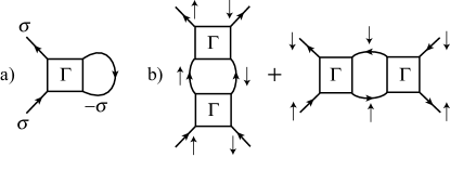
Figure 1: Feynman diagrams renormalizing a) the chemical potentials and b) the interatomic interaction.

However, when the Fermi mixture is critical, the inverse many-body vertex $\Gamma^{-1}_{{\bf 0},0}$ flows to zero according to the Thouless criterion and the chemical potentials in Eq. (3) diverge, which is unphysical. To go beyond this simple RG and calculate critical properties realistically, we need to take the frequency and momentum dependence of the interaction vertex into account, which are generated by the ladder and the bubble diagrams. The ladder diagram depends only on the external center-of-mass coordinates ${\bf q}$ and $\omega_{m}$, and its contribution to the renormalization of $\Gamma^{-1}_{{\bf q},m}$ is given by

$$\Xi(q^{2},i\omega_{m})=\int_{d\Lambda}d{\bf q^{\prime}}\frac{1-N_{\uparrow}(\epsilon_{\bf q^{\prime}})-N_{\downarrow}(\epsilon_{\bf q-q^{\prime}})}{-i\hbar\omega_{m}+\epsilon_{\bf q^{\prime}}+\epsilon_{\bf q-q^{\prime}}-2\mu}~{},$$ (4)

where during integration both ${\bf q^{\prime}}$ and ${\bf q-q^{\prime}}$ have to remain in the infinitesimal shell $d\Lambda$. Since the ladder diagram is already present at the two-body level, it is most important for scattering properties. Therefore, the interaction vertex is mainly dependent on the center-of-mass coordinates and we neglect the dependence of the vertex on other frequencies and momenta. The way to treat the external frequency and momentum dependence in wilsonian RG, is by expanding the (inverse) interaction in the following way: $\Gamma^{-1}_{{\bf q},m}=\Gamma^{-1}_{{\bf 0},0}-Z^{-1}_{q}q^{2}+Z^{-1}_{\omega}i\hbar\omega_{m}$. The flow equations for the additional coupling constants $Z_{q}^{-1}$ and $Z_{\omega}^{-1}$ are then obtained by considering the derivatives $\partial_{q^{2}}\Xi(q^{2},\omega)|_{q=\omega=0}$ and $\partial_{\omega}\Xi(q^{2},\omega)|_{q=\omega=0}$.

Extreme imbalance.— First, we apply the RG to one spin-down particle in a Fermi sea of spin-up particles at zero temperature in the unitarity limit. The full equation of state for the normal state of a strongly-interacting Fermi mixture was obtained at zero temperature using Monte-Carlo techniques Lobo . The most important feature of this equation is a so-called mean-field shift, caused by the strong interactions and characterized by a parameter $A$, which describes the self-energy of a single spin-down particle in a sea of spin-up particles Lobo ; Combescot . In this case, the RG equations are simplified, because $N_{\downarrow}$ can be set to zero and thus $\mu_{\uparrow}$ is not renormalized. Next, we have to incorporate the momentum and frequency dependence of the interaction in the one-loop Feynman diagram for the renormalization of $\mu_{\downarrow}$. In this particular case, the external frequency dependence of the ladder diagram can be taken into account exactly, since the one-loop Matsubara sum simply leads to the substitution $i\hbar\omega_{m}\rightarrow\epsilon_{\bf q}-\mu_{\uparrow}$ in Eq. (4) Combescot . The external momentum dependence is accounted for by the coupling $Z_{q}^{-1}$, giving

$$\frac{d\Gamma^{-1}_{{\bf 0},0}}{d\Lambda} = \frac{\Lambda^{2}}{2\pi^{2}}\left[\frac{1-N_{\uparrow}}{2\epsilon_{\Lambda}-\mu_{\downarrow}}-\frac{N_{\uparrow}}{2h}\right]~{},$$ (5)

$$\frac{d\mu_{\downarrow}}{d\Lambda} = \frac{\Lambda^{2}}{2\pi^{2}}\frac{N_{\uparrow}}{-\Gamma^{-1}_{{\bf 0},0}+Z^{-1}_{q}\Lambda^{2}}~{},$$ (6)

$$\frac{dZ^{-1}_{q}}{d\Lambda} = -\frac{\hbar^{4}\Lambda^{4}}{6\pi^{2}m^{2}}\frac{1-N_{\uparrow}}{(2\epsilon_{\Lambda}-\mu_{\downarrow})^{3}}~{},$$ (7)

where we note that these equations only have poles for positive values of $\mu_{\downarrow}$. Since this will not occur, we can simply use $\Lambda(l)=\Lambda_{0}e^{-l}$ to integrate out all momentum shells Bijlsma . We then obtain a system of three coupled ordinary differential equations in $l$, which are very easily solved numerically. If we take as an initial condition $\Gamma^{-1}_{{\bf 0},0}(0)=-m(\pi+2|a|\Lambda_{0})/4\pi^{2}|a|\hbar^{2}$ for a negative scattering length $a$, we automatically incorporate the relevant two-body physics exactly into our theory and also eliminate all dependence on the high-momentum cut-off $\Lambda_{0}$ Bijlsma . The unitarity limit is then given by $\Gamma^{-1}_{{\bf 0},0}(0)=-m\Lambda_{0}/2\pi^{2}\hbar^{2}$. The other initial conditions are $\mu_{\downarrow}(0)=\mu_{\downarrow}$ and $Z_{q}^{-1}(0)=0$, since the interaction starts out as being momentum independent. Note that in this calculation $\mu_{\downarrow}(0)=\mu_{\downarrow}$ is indeed negative and increases during the flow due to the strong attractive interactions. The quantum phase transition from a zero density to a nonzero density of spin-down particles occurs for the initial value $\mu_{\downarrow}$ that at the end of the flow precisely leads to $\mu_{\downarrow}(\infty)=0$. This happens when $\mu_{\downarrow}=-0.598\mu_{\uparrow}$, yielding $A=0.997$ in very good agreement with the Monte Carlo result $A=0.97(2)$ Lobo . This calculation also shows that it is crucial to let the chemical potential flow.

Phase diagram.— Next, we turn to our main topic, namely the critical properties of the strongly-interacting Fermi mixture and the calculation of the tricritical point in the phase diagram. Since it is not exact to make the substitution $\hbar\omega\rightarrow\epsilon_{\bf q}-\mu_{-\sigma}$ at nonzero temperatures, we take the frequency dependence of the ladder diagram into account through the renormalization of the coupling $Z^{-1}_{\omega}$. While the flow of $\Gamma^{-1}_{{\bf 0},0}$ is still given by Eq. (2), the expressions for the flow of $\mu_{\sigma}$ and $Z_{\omega}^{-1}$ become

$$\frac{d\mu_{\sigma}}{d\Lambda} = \frac{\Lambda^{2}}{2\pi^{2}}\frac{N_{-\sigma}+N_{\rm B}}{-\Gamma^{-1}_{{\bf 0},0}+Z^{-1}_{q}\Lambda^{2}-Z^{-1}_{\omega}(\epsilon_{\Lambda}-\mu_{-\sigma})}~{},$$ (8)

$$\frac{dZ^{-1}_{\omega}}{d\Lambda} = \frac{\Lambda^{2}}{2\pi^{2}}\frac{1-N_{\uparrow}-N_{\downarrow}}{4(\epsilon_{\Lambda}-\mu)^{2}}~{},$$ (9)

with $N_{\rm B}=1/\{\exp[\beta Z_{\omega}(-\Gamma^{-1}_{{\bf 0},0}+Z^{-1}_{q}\Lambda^{2})]-1\}$ coming from the bosonic frequency dependence of the interaction. A more cumbersome expression holds for $Z^{-1}_{q}$. The initial conditions are the same as for the extremely imbalanced case with in addition $\mu_{\uparrow}(0)=\mu_{\uparrow}$ and $Z^{-1}_{\omega}(0)=0$. As mentioned before, the critical condition is that the fully renormalized vertex $\Gamma^{-1}_{{\bf 0},0}(\infty)$, which can be seen as the inverse many-body T-matrix at zero external momentum and frequency, goes to zero. Physically, this implies that a many-body bound-state is entering the system. From Eq. (8), we see that incorporating the coupling constants $Z^{-1}_{q}$ and $Z^{-1}_{\omega}$, thereby taking the dependence of the interaction on the center-of-mass momentum and frequency into account, is crucial to solve the previously mentioned problem of the diverging chemical potential.

The only pole left in our set of RG equations is the average Fermi level $\mu=(\mu_{\uparrow}+\mu_{\downarrow})/2$, which is therefore the natural end point of our RG. However, this Fermi level is shifting due to the renormalization of the individual chemical potentials. This problem is conveniently solved by integrating out all momentum shells with the following procedure. First, we start at a high momentum cutoff $\Lambda_{0}$ and flow to a momentum $\Lambda^{\prime}_{0}$ at roughly two times the average Fermi momentum, with $k_{{\rm F}\sigma}=\sqrt{2m\epsilon_{{\rm F}\sigma}}/\hbar$. This integrates out the high-energy two-body physics, but hardly affects the chemical potentials. Then, we start integrating out the rest of the momentum shells symmetrically with respect to the flowing average Fermi level. This is achieved by using $\hbar\Lambda_{+}(l)/\sqrt{2m}=(\hbar\Lambda^{\prime}_{0}/\sqrt{2m}-\sqrt{\mu})e^{-l}+\sqrt{\mu(l)}$ and by $\hbar\Lambda_{-}(l)/\sqrt{2m}=-\sqrt{\mu}e^{-l}+\sqrt{\mu(l)}$. Note that as desired $\Lambda_{+}(l)$ starts at $\Lambda^{\prime}_{0}$ and automatically flows from above to $\sqrt{2m\mu(\infty)}/\hbar$, whereas $\Lambda_{-}(l)$ starts at 0 and automatically flows from below to $\sqrt{2m\mu(\infty)}/\hbar$.

We first apply the above procedure to study the equal density case, i.e., $h\rightarrow 0$, as a function of negative scattering length $a$. The scattering length enters the calculation through the initial condition of $\Gamma^{-1}_{{\bf 0},0}$. To express our results in terms of the Fermi energy $\epsilon_{\rm F}=\epsilon_{{\rm F}\sigma}$, we calculate the densities of atoms with the flow equation $dn_{\sigma}/d\Lambda=\Lambda^{2}N_{\sigma}/2\pi^{2}$. In the weak-coupling limit, $a\rightarrow 0^{-}$, the chemical potentials hardly renormalize, so that only Eq. (2) is relevant. The critical temperature becomes exponentially small, which allows us to solve Eq. (2) exactly with the result $k_{\rm B}T_{\rm c}=8\epsilon_{\rm F}e^{\gamma-3}\exp\{-\pi/2k_{\rm F}|a|\}/\pi$ and $\gamma$ Euler’s constant. Compared to the standard BCS-result we have an extra factor of $1/e$, coming from the screening effect of the bubble diagram that is not present in BCS theory. It is to be compared with the so-called Gor’kov correction, that reduces the critical temperature by a factor of 2.2 in the weak-coupling BCS-limit Heiselberg . The difference is due to the fact that we have only allowed for a nonzero center-of-mass momentum. This approximation is actually most appropriate in the unitarity limit and expected to be less accurate for weak coupling.

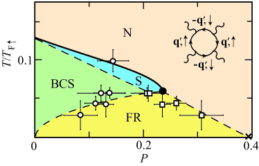
Figure 2: (Color online) The phase diagram of the homogeneous two-component Fermi mixture in the unitarity limit, consisting of the superfluid Sarma (S) and BCS phases, the normal phase (N) and the forbidden region (FR). The solid black line is the result of our RG calculations. The Monte-Carlo result of Lobo et al. Lobo , which is recovered by our RG, is indicated by a cross. The open circles and squares are data along the phase boundaries from the experiment of Shin et al. Shin . The dashed lines are only guides to the eye. Also shown is the Feynman diagram determining the tricritical point.

At larger values of $|a|$, the flow of the chemical potential becomes important and we obtain higher critical temperatures. In the unitarity limit, when $a$ diverges, we obtain $T_{\rm c}=0.13T_{\rm F}$ and $\mu(T_{\rm c})=0.55\epsilon_{\rm F}$ in good agreement with the Monte-Carlo results $T_{\rm c}=0.152(7)T_{\rm F}$ and $\mu(T_{\rm c})=0.493(14)\epsilon_{\rm F}$ Burovski . With our RG approach, we are in the unique position to accurately calculate the critical temperature as a function of polarization $P$ and compare with the recent experiment of Shin et al.. The result is shown in Fig. 2. The inset of this figure shows the one-loop diagram determining the position of the tricritical point. If it changes sign, then the fourth-order coefficient in the Landau theory for the superfluid phase transition changes sign and the nature of the phase transition changes from second order to first order. This yields $P_{\rm c3}=0.24$ and $T_{\rm c3}=0.06$ $T_{{\rm F}\uparrow}$ in good agreement with the experimental data. Our previous confirmation of the Monte-Carlo equation of state at $T=0$ implies that we also agree with the prediction of a quantum phase transition from the superfluid to the normal phase at a critical imbalance of $P_{\rm c}=0.39$ Lobo . Note that up to now, all theoretical predictions for the location of the tricritical point do not fit on the scale of Fig. 2. However, our calculations find good agreement with the experiments of Shin et al. in all limits.

Near the second-order phase boundary, the BCS order parameter $|\Delta|$ becomes arbitrarily small. Since at nonzero polarization we have that $h(\infty)>0$, it immediately follows that $h(\infty)>|\Delta|$. This means that the normal gas is unstable towards the so-called Sarma phase, which is a polarized superfluid with a gapless excitation spectrum for the majority spin-species Gubbels . However, the present RG is not suitable to calculate the full extent of the Sarma phase in the phase diagram or the precise shape of the forbidden region, because this requires a RG for the superfluid phase. The corresponding calculations are more involved than the present RG for the normal phase and is work in progress.

Acknowledgements. — We thank Tilman Enss and Pietro Massignan for useful discussions and Yong-il Shin for kindly providing us with the experimental data. This work is supported by the Stichting voor Fundamenteel Onderzoek der Materie (FOM) and the Nederlandse Organisatie voor Wetenschaplijk Onderzoek (NWO).

References

- (1) C. A. Regal et al., Phys. Rev. Lett. 92, 040403 (2004).
- (2) J. Carlson et al., Phys. Rev. Lett. 91, 050401 (2003).
- (3) G. E. Astrakharchik et al., Phys. Rev. Lett. 93, 200404 (2004).
- (4) E. Burovski et al., Phys. Rev. Lett. 96, 160402 (2006).
- (5) C. Lobo et al., Phys. Rev. Lett. 97, 200403 (2006).
- (6) C. A. Sá de Melo et al., Phys. Rev. Lett. 71, 3202 (1993).
- (7) R. Haussmann, Phys. Rev. B 49, 12975 (1994).
- (8) A. Perali et al., Phys. Rev. Lett. 92, 220404 (2004).
- (9) M. M. Parish et al., Nat. Phys. 3, 124 (2007).
- (10) H. Hu et al., Nat. Phys. 3, 469 (2007).
- (11) Y. Nishida and D. T. Son, Phys. Rev. Lett. 97, 050403 (2006).
- (12) P. Nikolić and S. Sachdev, Phys. Rev. A 75, 033608 (2007).
- (13) M. Y. Veillette et al., Phys. Rev. A 75, 043614 (2007).
- (14) M. C. Birse et al., Phys. Lett. B 605, 287 (2005).
- (15) S. Diehl et al., Phys. Rev. A 76, 021602(R) (2007).
- (16) K. G. Wilson and J. Kogut, Phys. Rep. 12, 75 (1974).
- (17) R. Shankar, Rev. Mod. Phys. 66, 129 (1994).
- (18) C. Honerkamp et al., Phys. Rev. B 63, 035109 (2001).
- (19) P. Kopietz and T. Busche, Phys. Rev. B 64, 155101 (2001).
- (20) M. W. Zwierlein et al., Science 311, 492 (2006).
- (21) G. B. Partridge et al., Science 311, 503 (2006).
- (22) K. B. Gubbels et al., Phys. Rev. Lett. 97, 210402 (2006).
- (23) G. B. Partridge et al., Phys. Rev. Lett. 97, 190407 (2006).
- (24) M. Haque and H. T. C. Stoof, Phys. Rev. Lett. 98, 260406 (2007).
- (25) Y. Shin et al., Nature 451, 689 (2008).
- (26) R. Combescot et al., Phys. Rev. Lett. 98, 180402 (2007).
- (27) M. Bijlsma and H. T. C. Stoof, Phys. Rev. A 54, 5085 (1996).
- (28) H. Heiselberg et al., Phys. Rev. Lett. 85, 2418 (2000).