Persistent current and Wigner crystallization in a one dimensional quantum ring

Abstract

We use Density Functional Theory to study interacting spinless electrons on a one-dimensional quantum ring in the density range where the system undergoes Wigner crystallization. The Wigner transition leads to a drastic “collective” electron localization due to the Wigner crystal pinning, provided a weak impurity potential is applied. To reveal this localization we examine a persistent current in a ring penetrated by a magnetic flux. Using the DFT-OEP method we calculated the current as a function of the interaction parameter $r_{\rm S}$. We find that in the limit of vanishing impurity potential the persistent current stays constant up to a critical value of $r_{\rm S}^{\rm c}\approx 2.05$ but shows a drastic exponential decay for larger $r_{\rm S}$ which reflects a formation of a pinned Wigner crystal. Above $r_{\rm S}^{\rm c}$ the amplitude of the electron density oscillations exactly follows the $(r_{\rm S}-r_{\rm S}^{\rm c})^{{}^{1}/_{2}}$ behaviour, confirming a second-order phase transition as expected in the mean-field-type OEP approximation.

I Introduction

In the last years, the fabrication of quasi-one-dimensional quantum rings became possible Ihn et al. (2003); Mailly et al. (1993). In such systems only few transverse states are occupied and by increasing the curvature of the confining potential the system can be made effectively one-dimensional. The number of electrons on the ring can be controlled by the gate electrode. The experimental studies of the rings with only one or two electrons were reported by Lorke et al. Lorke et al. (2000) The possibility to vary the number of particles from very few to several hundreds enables experimentalists to tune the electron-electron interaction in a wide range. One of the most striking consequences of the interaction is the formation of a Wigner crystal Wigner (1934), a many-body state with electrons localized at discrete lattice sites. Yet it is well known that in an infinite one-dimensional system the fluctuations destroy the long-range orderLandau and Lifschitz (1969). This raised doubts about the existence of a one-dimensional Wigner crystal which has become a long-debated subject. Only in the nineties Glazman et al. Glazman et al. (1992) have shown that the arbitrarily weak pinning potential stabilizes the one-dimensional Wigner crystal. It was proven that the pinning potential suppresses the long-wavelength fluctuation modes which are responsible for destroying the long-range order. Due to the pinning potential the Wigner state is always localized in contrast to the electron liquid state Glazman et al. (1992). Thus in the presence of a weak impurity the Wigner transition should manifest itself as electron localization.

The critical $r_{\rm S}^{\rm c}$ for a 1D system estimated in the work of Glazman et al. was of the order of unity. For the two-dimensional electron gas Tanatar and Ceperley found a critical value $r_{\rm S}^{\rm c}=37\pm 5$, using a Monte-Carlo technique Tanatar and Ceperley (1989). The reason for this large value is a very small shear modulus of the two-dimensional Wigner crystal Glazman et al. (1992). In three dimensions a Wigner crystal is expected at $r_{\rm S}>65\pm 10$ (Ref. Ortiz et al., 1999).

Electron localization seems to be a convenient signature to observe a formation of the pinned one-dimensional Wigner crystal. However, in numerical simulations it is not quite evident how to quantify the localization of a correlated many body state. Several indirect criteria such as the inverse participation number Kramer and MacKinnon (1993) or the curvature of the ground state energy Kohn (1964) have been suggested to distinguish between a localized and a delocalized state. However, to the best of our knowledge, the electrons’ ability to carry electric current – which is the most direct indication of the delocalized vs. localized behaviour – has not yet been explored. In this work we calculate the persistent current in a one-dimensional quantum ring penetrated by a magnetic flux. We apply a weak impurity potential which pins a Wigner state but practically does not influence the electron liquid state.

In the density range where a Wigner crystal already exists as a ground state the persistent current has been studied analytically by Krive et al.Krive et al. (1995) for smooth potentials allowing semiclassical treatment. In a perfect ring the Wigner crystal rotates as a whole producing exactly the same current as non-interacting electrons. In the presence of a weak impurity potential the persistent current was found to be suppressed exponentially with the increasing impurity strength or the Wigner crystal stiffness Krive et al. (1995).

We use Density Functional Theory (DFT) to calculate self-consistently the persistent current in a one-dimensional system with ten electrons. In the limit of vanishing (on a scale of the inter-electron Coulomb repulsion) repulsive potential we find that the current is independent of $r_{\rm S}$ for $r_{\rm S}<2.05$. At larger $r_{\rm S}$ the persistent current decreases exponentially with increasing $r_{\rm S}$, indicating a localization of the electrons. At the transition point the system undergoes a second-order phase transition which can be seen by considering the amplitude of the density oscillations $\delta$ as an order parameter. We find that in a crystalline phase $\delta$ exactly follows a square root behaviour $\delta\sim\left(r_{\rm S}-r_{\rm S}^{\rm c}\right)^{{}^{1/_{2}}}$. The stronger pinning potentials smear the phase transition such that no distinct transition point can be observed.

The article is organized as follows. In section II we introduce the model of a one-dimensional quantum ring with the Gaussian impurity potential. We briefly discuss the OEP approximation Sharp and Horton (1953); Talman and Shadwick (1976) which is used for the exchange potential. We also introduce an Electron Localization Function Becke and Edgecombe (1990) which is helpful for a real-space visualization of the electron localization. In section III we describe the computational method for solving the self-consistent Kohn-Sham equations. In section IV we present our results for the persistent current as a function of $r_{\rm S}$. We consider impurity potentials of various amplitude and width and show how these parameters influence the current. The conclusions are given in section V.

II The model

We study a system of $N=10$ interacting spinless electrons in a one dimensional ring of circumference $L=2\pi R$. The ring geometry is accounted for via periodic boundary conditions and $x=\varphi R$ denotes the coordinate along the ring. A persistent current is induced by a vector potential $\vec{A}=(A_{r},A_{\varphi})$ with a tangential component

$$A_{\varphi}=\frac{\Phi}{L}$$ (1)

that provides a magnetic flux $\Phi$ through the ring. The vector potential is chosen such that the electrons move in a field-free space.

Additionally, we introduce a repulsive Gaussian potential centered at $x_{0}$

$$V_{\rm imp}(x)=V_{0}\exp\left(-\frac{(x-x_{0})^{2}}{\sigma^{2}}\right),\hskip 30.00005pt(V_{0}>0)$$ (2)

which should pin the Wigner crystal phase.

We calculate the ground state current density for a given value of the magnetic flux and for a given strength and width of the impurity potential using Density Functional Theory. The self consistent Kohn-Sham Kohn and Sham (1965) equations for this system are given by

$$\left[\frac{1}{2m_{0}^{\ast}}\left(-i\hbar\partial_{x}-eA_{\varphi}\right)^{2}+V_{\rm imp}(x)+V_{\rm int}(x)\right]\varphi_{i}(x)\\ =\epsilon_{i}\varphi_{i}(x)$$ (3)

where index $i$ labels the Kohn-Sham orbitals $\varphi_{i}$ and the eigenvalues $\epsilon_{i}$. The electron-electron interaction is described by an effective one-particle scalar potential $V_{\rm int}=V_{\rm H}+V_{\rm OEP}^{\rm x}$. Here, $V_{\rm H}$ is the Hartree potential and $V_{\rm OEP}^{\rm x}$ is the exchange contribution. The latter is calculated in the KLI version Krieger et al. (1992a, b) of the OEP method Sharp and Horton (1953); Talman and Shadwick (1976).

The central assumption of the OEP method is that the exchange-correlation energy functional can be written explicitely in terms of the Kohn-Sham orbitals. A common choice is the “exact exchange” functional

$$E_{\rm x}^{\rm EXX}=-\frac{1}{2}\frac{e^{2}}{4\pi\varepsilon\varepsilon_{0}}\sum_{i,j}^{N}\iint dx\,dx^{\prime}\,\frac{\varphi^{\ast}_{i}(x)\varphi_{j}(x)\varphi^{\ast}_{j}(x^{\prime})\varphi_{i}(x^{\prime})}{|x-x^{\prime}|}$$ (4)

which has the form of the Fock energy but the wavefunctions $\varphi_{i}$ are the Kohn-Sham orbitals rather than the Hartree-Fock orbitals. Minimization of the full energy functional with respect to the density leads to an integral equation for the exchange-correlation potential. In this work we use the exact-exchange functional and apply the KLI approximation which allows to transform the OEP integral equation into a considerably simpler algebraic equation. Still, it retains important features of the exact xc potential such as the derivative discontinuities and correct asymptotic behaviour Grabo et al. (2000).

Since DFT in the Kohn-Sham formulation is essentially a mean-field theory, fluctuations are not accounted for in our calculations. It is well known that fluctuations are particularly important in one dimension Landau and Lifschitz (1969). But since even an infinite one-dimensional Wigner crystal is stabilized by an arbitrarily weak pinning potential Glazman et al. (1992) we expect that the fluctuations are effectively suppressed not only due to the pinning potential, but also due to the finite size of the ring.

Whether the ground state of a many electron system is an electron gas-like one or a Wigner crystal state depends on the ratio of the kinetic energy and the Coulomb energy. In one dimension this ratio is simply proportional to the electron density $n$, whereas in two and three dimensions it is proportional to $\sqrt{n}$ and $n^{{}^{1}/_{3}}$, respectively. Hence for high densities the kinetic energy dominates and the ground state is electron gas-like whereas for low densities the Coulomb repulsion favours the crystalline state.

Experimentally it is most straightforward to vary the electron density to switch between weakly and strongly interacting regimes. Yet the variation of the electron number should alter the persistent current even in a non-interacting system which conceals the interaction effects. As we use a “persistent current criterion” to identify the Wigner transition we prefer to exclude the aforementioned trivial single particle contribution and to retain only the influence of many-body effects. It can be done using an alternative (though somewhat artificial) way of controlling the ratio of kinetic and Coulomb energy. Namely, let us consider the effective electron mass $m^{\ast}$ as a free parameter. In one dimension, the energy ratio $r_{\rm S}$ is proportional to $m^{\ast}$:

$$r_{\rm S}=\frac{1}{2N}\frac{L}{a_{\rm B}}\frac{m^{\ast}}{m_{0}^{\ast}}\,{,}$$ (5)

where $a_{\rm B}$ and $m_{0}^{\ast}$ are the Bohr radius and the “true” effective electron mass in the host material. The persistent current density

$$j(x)=-\frac{i\hbar}{2m_{0}^{\ast}}\sum_{i=1}^{N}\left[\varphi_{i}^{\ast}(x)\partial_{x}\varphi_{i}(x)-\varphi_{i}(x)\partial_{x}\varphi_{i}^{\ast}(x)\right]\\ -\frac{\hbar}{m_{0}^{\ast}}\frac{2\pi}{L}\frac{\Phi}{\Phi_{0}}n(x)$$ (6)

should be calculated with the fixed “true” effective electron mass $m_{0}^{\ast}$. Here, $\Phi_{0}=\frac{h}{e}$ is the flux quantum and

$$n(x)=\sum_{i=1}^{N}\varphi_{i}^{\ast}(x)\varphi_{i}(x)$$ (7)

is the density.

Also, the ratio of the kinetic energy to the impurity potential must be kept constant when changing $r_{\rm S}$ via changing $m^{\ast}$. Otherwise the current density of a system of non-interacting electrons would depend on $r_{\rm S}$. The impurity potential strength $V_{0}$ must be renormalized as

$$V_{0}\rightarrow V_{0}^{\ast}=V_{0}\frac{m_{0}^{\ast}}{m^{\ast}}\,{.}$$ (8)

The potential renormalization (8) guarantees that the artificial variation of the electron mass results in a dependence of the persistent current on $r_{\rm S}$ solely due to the electron-electron interaction.

Equation (6) expresses the current density via the Kohn-Sham orbitals within the framework of the ordinary density-based DFT. It is not, however, strictly justified since the common DFT Kohn-Sham equations by construction yield the exact ground state density but not the current density. Strictly speaking, one has to employ the current density functional theory Vignale and Rasolt (1988) (CDFT) which expresses the ground-state energy functional as a functional of the density and the paramagnetic current density. The Kohn-Sham orbitals in CDFT thus give the exact current density of the interacting system. However, the CDFT corrections are, as a matter of fact, usually very small. For example in a recent paper Sharma et al. (2007) is shown that the orbital magnetic moments in magnetic (Fe, Co and Ni) and non-magnetic (Si and Ge) solids calculated with CDFT only slightly differ from those calculated with DFT. Hence we expect that Eq. (6) evaluates the current reasonably well, keeping in mind, that for our purposes not the current value itself, but its critical $r_{\rm S}$-dependence close to the Wigner transition is of interest.

In addition to the current density we also use the Electron Localization Function (ELF) Becke and Edgecombe (1990) to visualize the electrons’ localization. The idea behind the definition of the ELF is that the more localized electron produces a stronger repulsion of the other like-spin electrons due to the Pauli exclusion principle. According to this picture the ELF measures the probability to find a second electron (with the parallel spin) anywhere close to a reference electron. It is defined such that its value of one half means a homogeneous electron-gas like state whereas a value of one refers to a perfectly localized electron at this point in space.

In its original definition Becke and Edgecombe (1990) the ELF was formulated for the real wavefunctions only. Recently it was generalized to the time-dependent case Burnus et al. (2005) where complex wavefunctions have to be employed. This form of the ELF is also suitable for the current-carrying static system we consider. It is given by

$$\eta(x)=\frac{1}{1+\chi^{2}(x)}$$ (9)

with

$$\chi(x)=\frac{\tau(x)-\frac{1}{4}\frac{(n^{\prime}(x))^{2}}{n(x)}-\frac{(j_{\rm p}(x))^{2}}{n(x)}}{\tau^{\rm hom}(x)}\,{.}$$ (10)

In this expression $\tau(x)=\frac{\hbar^{2}}{m_{0}^{\ast}}\sum_{i}|\partial_{x}\varphi_{i}(x)|^{2}$ is the kinetic energy density of the Kohn-Sham system and $\tau^{\rm hom}(x)=\frac{\hbar^{2}\pi^{2}}{6m_{0}^{\ast}}n^{3}(x)$ is the respective quantity in a one-dimensional homogeneous electron gas with density $n(x)$.

III Computational method

For numerical solution of the Kohn-Sham equations (3) we use a real space method. We expand the wave functions $\varphi_{i}(x)$ using a spline basis Hofmann et al. (2001)

$$\varphi_{i}(x)=\sum_{\nu}a_{i}^{(\nu)}b_{\nu}(x)$$ (11)

with the complex coefficients $a_{i}^{(\nu)}$ and the real basis functions

$$b_{\nu}(x)=\left\{\begin{array}[]{r@{\quad:\quad}l}\frac{1}{4}\left(2+\frac{x-x_{\nu}}{h}\right)^{3}&-2<\frac{x-x_{\nu}}{h}\leq-1\\[2.15277pt] 1-\frac{3}{2}\left(\frac{x-x_{\nu}}{h}\right)^{2}-\frac{3}{4}\left(\frac{x-x_{\nu}}{h}\right)^{3}&-1<\frac{x-x_{\nu}}{h}\leq 0\\[2.15277pt] 1-\frac{3}{2}\left(\frac{x-x_{\nu}}{h}\right)^{2}+\frac{3}{4}\left(\frac{x-x_{\nu}}{h}\right)^{3}&0<\frac{x-x_{\nu}}{h}\leq 1\\[2.15277pt] \frac{1}{4}\left(2-\frac{x-x_{\nu}}{h}\right)^{3}&1<\frac{x-x_{\nu}}{h}\leq 2\\[2.15277pt] 0&\textrm{else.}\end{array}\right.$$ (12)

The spline nodes are $x_{\nu}$ and $h$ is the distance between the two adjacent nodes. The basis functions (12) are not orthogonal which means that the overlap matrix

$$S_{\mu,\nu}=\int dx\,b_{\mu}(x)b_{\nu}(x)$$ (13)

is not diagonal. With this representation of the wave functions, the Schrödinger equation reads

$$\sum_{\nu}H_{\mu,\nu}a_{i}^{(\nu)}=\epsilon_{i}\sum_{\nu}S_{\mu,\nu}a_{i}^{(\nu)}$$ (14)

with the Hamiltonian matrix

$$H_{\mu,\nu}=\int dx\,b_{\mu}(x)\hat{H}b_{\nu}(x)\,{.}$$ (15)

At the first step this generalized eigenvalue equation is transformed into a standard eigenvalue equation. We use a Cholesky decomposition Press et al. (1996) of the overlap matrix

$$\hat{S}=\hat{L}\hat{L}^{\rm T}$$ (16)

into a lower triangular matrix $\hat{L}$ and its transpose and write the eigenvalue equation as

$$\hat{L}^{-1}\hat{H}\left(\hat{L}^{\rm T}\right)^{-1}\hat{L}^{\rm T}\vec{a}_{i}=\epsilon_{i}\hat{L}^{\rm T}\vec{a}_{i}\,{.}$$ (17)

The matrix $\hat{L}^{-1}\hat{H}\left(\hat{L}^{\rm T}\right)^{-1}$ is diagonalized using the zheev-routine form the LAPACK library Anderson et al. (1999) and the resulting eigenvector $\hat{L}^{\rm T}\vec{a}_{i}$ is transformed back to obtain the eigenvector $\vec{a}_{i}$ of the original generalized eigenvalue problem.

The starting point for the iterative self-consistent procedure is a system of non-interacting particles i.e. a system with $V_{\rm H}=V_{\rm x}=0$. The resulting non-interacting eigenfunctions are then used to construct the first approximation for the Hartee- and the exchange potential. In the subsequent iterations the Hartree- and the exchange potential are calculated from the eigenfunctions of the previous step . As a measure of the convergence we consider the maximum difference between two Kohn-Sham eigenvalues in the $n$-th and $(n-1)$-th iteration step:

$$\max_{i}\left|\varepsilon_{i}^{(n)}-\varepsilon_{i}^{(n-1)}\right|<\Delta\,{.}$$ (18)

We found that this difference has to be extremely small compared to the Kohn-Sham eigenvalues themselves which are of the order of several tens of meV, namely $\Delta\approx 10^{-10}$meV. The reason for this very small number are low energy excitations which correspond to a charge displacement over a large distance in the system. If the chosen $\Delta$ is too large, one encounters a density range where the system seems to be in a delocalized state whereas in fact it becomes localized after the solution is converged. Generally, a very high computational accuracy is required to distinguish correctly between a localized and a delocalized state of the system.

IV Results

In this section we present the results of our calculations of the persistent current in the one-dimensional quantum ring. For the effective electron mass and the dielectric constant we have chosen the GaAs values $m_{0}^{\ast}=0.0665m_{\rm e}$ and $\epsilon=12.5$. The value of the magnetic field flux was chosen as $\Phi=0.3\Phi_{0}$. In fact, the particular magnitude of the flux does not matter provided the current distinctly exceeds numerical inaccuracy.

For the Wigner crystal pinning we apply a narrow impurity potential of a width $\sigma=0.025L$ much smaller than the average distance between electrons $\frac{L}{N}=0.1L$. The persistent current is calculated as a function of $r_{\rm S}$, the latter being altered by varying $m^{\ast}$, according to Eqs. (5), (8). The current is normalized to its value $j_{0}$ for non-interacting electrons in the presence of an impurity potential with unrenormalized strength $V_{0}=10^{-3}$meV. The results for various impurity potential strengths are shown in Fig. 1. The dashed line $\frac{j}{j_{0}}=1$ reflects the current independence of $r_{\rm S}$ for noninteracting electrons.

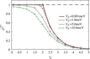
Figure 1: (Color online) The persistent current as a function of $r_{\rm S}$ for a Gaussian impurity potential with a half maximum width of $2.5\%$ of the ring circumference. The current is normalized to its value $j_{0}$ in a non-interacting system and potential strength $V_{0}=10^{-3}$meV. The long-dashed line ${}^{j}/_{j_{0}}=1$ corresponds to the interaction-free system.

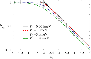
Figure 2: (Color online) Logarithmic version of the plot in Fig. 1. The exponential dependence of the persistent current on $r_{\rm S}$ is clearly seen.

As seen in Fig. 1 for the smallest $V_{0}=10^{-3}$ meV, one can clearly distinguish two different regions of $r_{\rm S}$. Below the critical value of $r_{\rm S}^{\rm c}\approx 2.05$, the persistent current is independent of $r_{\rm S}$. Its magnitude is the same as in the non-interacting system which means that the interacting system is electron gas-like. In contrast, for $r_{\rm S}>r_{\rm S}^{\rm c}$, the persistent current drops exponentially with increasing $r_{\rm S}$ which is seen explicitely from the linear dependence of $\log^{j}/_{j_{0}}$ on $r_{\rm S}$ shown in Fig. 2. This signifies the formation of the Wigner crystal pinned by an extremely small impurity potential. Hence the value $r_{\rm S}^{\rm c}=2.05$ can be interpreted as a critical $r_{\rm S}$ of the Wigner transition.

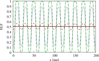
Figure 3: (Color online) Electron Localization Function in the presence of a weak ($V_{0}=0.001$meV) potential. Shown is the ELF for different values of $r_{\rm S}$. Solid line: $r_{\rm S}=0.1$, dashed line: $r_{\rm S}=2.06$, dotted line: $r_{\rm S}=2.5$, dash-dotted line: $r_{\rm S}=5.0$. An ELF value of one corresponds to perfect localization whereas an ELF value of one half means homogeneous electron gas-like delocalization.

This interpretation is supported by the ELF plot in Fig. 3. For $r_{\rm S}\leq 2.05$ we find an ELF value of one half, corresponding to completely delocalized electrons. This changes drastically when $r_{\rm S}$ exceeds $r_{\rm S}^{\rm c}$. With increasing $r_{\rm S}$ the electrons tend to localize at discrete lattice sites. At $r_{\rm S}\approx 5$ they arrange in an “almost classical” one-dimensional lattice. The complete localization is achieved within a rather narrow interval of $r_{\rm S}$ as exemplified in Fig. 3 by the ELF graphs for $r_{\rm S}=2.06$ and $r_{\rm S}=2.5$. This reflects the exponential decay of the persistent current as shown in Fig. 1.

We believe, that within our numerical accuracy the solid curve in Fig. 1 corresponds to the case of the “vanishing” external potential. Such a potential does not disturb the Wigner transition, but provides the pinning. The particular potential strength and width should be then unimportant. We tested this calculating the current density for several values of the width of the pinning potential (all with $V_{0}=10^{-3}$meV) and found that the persistent current follows exactly the same $r_{\rm S}$-dependence. However, the convergence is getting much harder for wider potentials since the “smoother” potentials are less effective in pinning the Wigner crystal. For $V_{0}$ values below $10^{-3}$meV the convergence could not be reached. Yet using a semiclassical approach Krive et al. (1995) it can be shown analytically that the current value $j_{0}$ of a non-interacting system is indeed recovered for $V_{\rm imp}=0$.

The critical $r_{\rm S}^{\rm c}=2.05$ we obtained in this work is of the same order as the values for $r_{\rm S}^{\rm c}$ found in a previous work Hofmann (2005) for a different model using the ground state energy curvature Kohn (1964) as a localization criterion. In the presence of a disorder potential with an amplitude $\Delta V=0.02$meV a Wigner transition has been observed in the range $2.08\leq r_{\rm S}^{\rm c}\leq 5.04$ depending on the model for the electron-electron interaction.

The other three curves in Fig. 1 show the current of the interacting system for $V_{0}=1.0$meV, $V_{0}=5.0$meV and $V_{0}=10.0$meV. Although at $V_{0}=1.0$meV there is still the range of $r_{\rm S}$ where $j=j_{\rm 0}$, the sharp kink at $r_{\rm S}=r_{\rm S}^{\rm c}$ vanishes. The transition smoothing is more pronounced for $V_{0}=5.0$meV and $V_{0}=10.0$meV where no region of $r_{\rm S}$ where the current is independent of $r_{\rm S}$ is seen.

It should be emphasized that the dependence of the normalized current on $r_{\rm S}$ is solely due to the electron-electron interaction. The smooth decrease of the current with increasingly strong Coulomb interaction observed for stronger impurity potentials ($V_{0}=5.0$meV and $V_{0}=10.0$meV) reflects a gradual localization of the many-body state instead of a distinct phase transition. This behaviour parallels the absence of a sharp phase transition in an external potential field that lowers the symmetry of the high-symmetry phase Landau and Lifschitz (1969).

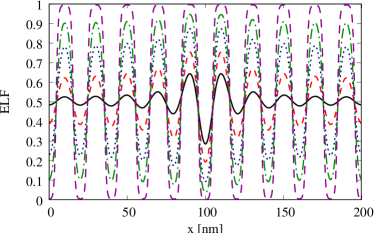
Figure 4: (Color online) Electron Localization Function in the presence of an intermediate ($V_{0}=5.0$meV) narrow potential. Shown is the ELF for different values of $r_{\rm S}$. Solid line: $r_{\rm S}=0.1$, dashed line: $r_{\rm S}=1.5$, dotted line: $r_{\rm S}=2.0$, dash-dotted line: $r_{\rm S}=2.5$, long-dashed line: $r_{\rm S}=5.0$. For intermediate values of $r_{\rm S}$ the electrons next to the impurity are more localized. This localization increases gradually with increasing $r_{\rm S}$. For large values of $r_{\rm S}$ the ELF is the same as found in the case of the weak potential (see Fig 3).

An estimate of the Coulomb energy of two electrons at a distance $d=\frac{L}{N}=20.0$nm

$$U=\frac{e^{2}}{4\pi\varepsilon\varepsilon_{0}}\frac{1}{d}\approx 5.75\text{meV}$$ (19)

shows that it is indeed of the order of the pinning potential which smoothes out the phase transition and induces a gradual localization. For $V_{0}\geq 1$meV and at intermediate values of $r_{\rm S}$ it can be seen directly from the ELF plots (Fig. 4) that the localization is more pronounced next to the pinning potential. This indicates that a gradual localization seen in Fig. 1 is driven by the interplay between the long-range Coulomb repulsion and the interaction with the short-range impurity potential, both being of the same order.

The sharp transition we found for a “vanishing” impurity potential (solid line in Fig. 1) is a second order phase transition from an electron liquid state to the Wigner crystal state. This can be verified by plotting the $r_{\rm S}$-dependence of the order parameter $\delta$ which shows a behaviour $\delta\sim\left(r_{\rm S}-r_{\rm S}^{\rm c}\right)^{{}^{1}/_{2}}$ at $r_{\rm S}>r_{\rm S}^{\rm c}$, i.e. in the low-symmetry phase Landau and Lifschitz (1969). Indeed, taking the amplitude of the density oscillations as the order parameter $\delta$, we obtain an exact square root dependence, as shown in Fig. 5. The second-order type of the transition we observe in our calculations is quite natural for the mean-field-type DFT-OEP approach.

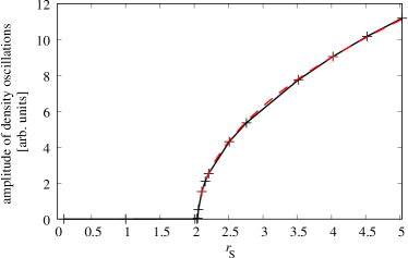
Figure 5: (Color online) Amplitude of the density oscillations as a function of $r_{\rm S}$ for a weak impurity potential ($V_{0}=0.001$meV). The solid black curve shows the calculated data, the dashed red curve is a square root $\left(r_{\rm S}-r_{\rm S}^{\rm c}\right)^{{}^{1}/_{2}}$ behaviour.

From the exponential dependence of the current on $r_{\rm S}$ (Fig. 1) we can deduce the relation between the persistent current density and the order parameter

$$j(\delta)=j_{0}\exp(-\alpha\delta^{2})$$ (20)

where the numerical factor $\alpha=0.033L^{2}$.

V Conclusions

In this article we investigated numerically the influence of the electron-electron interaction on the ground state of a one-dimensional electron gas confined in a ring geometry. To break the rotational invariance of the ring we introduce a weak “impurity” potential. This potential does not affect the delocalized electron liquid phase, but provides a pinning of the crystalline Wigner phase. We employ a persistent current in the ring as a measure of the Wigner crystal pinning. For a sufficiently weak impurity potential we found that for $r_{\rm S}<r_{\rm S}^{\rm c}$ the current density of the interacting system is exactly the same as the current density of a non-interacting electron gas. For $r_{\rm S}>r_{\rm S}^{\rm c}$ the current of the interacting system decays exponentially with increasing $r_{\rm S}$ while the current of a non-interacting system remains constant. This behaviour clearly shows the formation of the Wigner crystal in a one-dimensional system. This interpretation is confirmed by the ELF plots which reveal the delocalized electron distribution below the critical $r_{\rm S}^{\rm c}$ and a localized one above $r_{\rm S}^{\rm c}$. At $r_{\rm S}=r_{\rm S}^{\rm c}$ the system undergoes a second-order phase transition from an electron liquid to a Wigner crystal. This is evident from the square root dependence of the amplitude of the density oscillations (taken as the order parameter) on $r_{\rm S}$ above the critical value. Experimentally, this transition should be observable as a sharp decrease of the ring’s magnetization when the electron density is lowered. However, in a real experiment this transition will be superposed with the interaction-independent variation of the current density due to the variation of the particle number. The critical value $r_{\rm S}^{\rm c}=2.05$ we find for the Wigner transition is consistent with the density rangeGlazman et al. (1992) in which Glazman et al. expected the existence of a stable one-dimensional Wigner crystal.

References

- Ihn et al. (2003) T. Ihn, A. Fuhrer, T. Heinzel, K. Ensslin, W. Wegscheider, and M. Bichler, Physica E Low-Dimensional Systems and Nanostructures 16, 83 (2003).
- Mailly et al. (1993) D. Mailly, C. Chapelier, and A. Benoit, Phys. Rev. Lett. 70, 2020 (1993).
- Lorke et al. (2000) A. Lorke, R. Johannes Luyken, A. O. Govorov, J. P. Kotthaus, J. M. Garcia, and P. M. Petroff, Phys. Rev. Lett. 84, 2223 (2000).
- Wigner (1934) E. Wigner, Phys. Rev. 46, 1002 (1934).
- Landau and Lifschitz (1969) L. Landau and E. Lifschitz, Course of theoretical physics, vol. V,Statistical physics (Pergamon Press, London, 1969), 2nd ed.
- Glazman et al. (1992) L. I. Glazman, I. M. Ruzin, and B. I. Shklovskii, Phys. Rev. B 45, 8454 (1992).
- Tanatar and Ceperley (1989) B. Tanatar and D. M. Ceperley, Phys. Rev. B 39, 5005 (1989).
- Ortiz et al. (1999) G. Ortiz, M. Harris, and P. Ballone, Phys. Rev. Lett. 82, 5317 (1999).
- Kramer and MacKinnon (1993) B. Kramer and A. MacKinnon, Reports on Progress in Physics 56, 1469 (1993), URL http://stacks.iop.org/0034-4885/56/1469.
- Kohn (1964) W. Kohn, Phys. Rev. 133, A171 (1964).
- Krive et al. (1995) I. V. Krive, P. Sandström, R. I. Shekhter, S. M. Girvin, and M. Jonson, Phys. Rev. B 52, 16451 (1995).
- Sharp and Horton (1953) R. T. Sharp and G. K. Horton, Phys. Rev. 90, 317 (1953).
- Talman and Shadwick (1976) J. D. Talman and W. F. Shadwick, Phys. Rev. A 14, 36 (1976).
- Becke and Edgecombe (1990) A. D. Becke and K. E. Edgecombe, J. Chem. Phys. 92, 5397 (1990).
- Kohn and Sham (1965) W. Kohn and L. J. Sham, Physical Review 140, A1133 (1965).
- Krieger et al. (1992a) J. B. Krieger, Y. Li, and G. J. Iafrate, Phys. Rev. A 45, 101 (1992a).
- Krieger et al. (1992b) J. B. Krieger, Y. Li, and G. J. Iafrate, Phys. Rev. A 46, 5453 (1992b).
- Grabo et al. (2000) T. Grabo, T. Kreibich, S. Kurth, and E. K. U. Gross, in Strong Coulomb correlations in electronic structure calculations: beyond the Local Density Approximation, edited by V. Anisimov (Gordon and Breach, Amsterdam, 2000).
- Vignale and Rasolt (1988) G. Vignale and M. Rasolt, Phys. Rev. B 37, 10685 (1988).
- Sharma et al. (2007) S. Sharma, S. Pittalis, S. Kurth, S. Shallcross, J. K. Dewhurst, and E. K. U. Gross, Physical Review B (Condensed Matter and Materials Physics) 76, 100401 (pages 4) (2007), URL http://link.aps.org/abstract/PRB/v76/e100401.
- Burnus et al. (2005) T. Burnus, M. A. L. Marques, and E. K. U. Gross, Physical Review A (Atomic, Molecular, and Optical Physics) 71, 010501 (pages 4) (2005), URL http://link.aps.org/abstract/PRA/v71/e010501.
- Hofmann et al. (2001) M. Hofmann, M. Bockstedte, and O. Pankratov, Phys. Rev. B 64, 245321 (2001).
- Press et al. (1996) W. H. Press, S. A. Teukolsky, W. T. Vetterling, and B. P. Flannery, Numerical Recipes in C (Cambride University Press, Cambridge, 1996).
- Anderson et al. (1999) E. Anderson, Z. Bai, C. Bischof, S. Blackford, J. Demmel, J. Dongarra, J. Du Croz, A. Greenbaum, S. Hammarling, A. McKenney, et al., LAPACK Users’ Guide (Society for Industrial and Applied Mathematics, Philadelphia, PA, 1999).
- Hofmann (2005) M. Hofmann, Ph.D. thesis, Universität Erlangen-Nürnberg (2005).