Abstract

In this article, we calculate the electromagnetic form-factor of the $\pi$ meson with the light-cone QCD sum rules. The numerical value $F_{\pi}^{p}(0)=0.999\pm 0.001$ is in excellent agreement with the experimental data (extrapolated to the limit of zero momentum transfer, or the normalization condition $F_{\pi}(0)=1$). For large momentum transfers, the values from the two sum rules are all comparable with the experimental data and theoretical estimations.

PACS numbers: 12.38.Lg; 13.40.Gp

Key Words: Electromagnetic form-factor, Light-cone QCD sum rules

1 Introduction

The $\pi$ meson, as both Nambu-Goldstone boson and quark-antiquark bound state, plays an important role in testing the quark models and exploring the low energy QCD. Its electromagnetic form-factor and electromagnetic radius are important parameters, and have been extensively studied both experimentally [1, 2, 3, 4, 5, 6, 7] and theoretically, for examples, the QCD sum rules [8, 9, 10, 11], the light-cone QCD sum rules [12, 13, 14, 15], perturbative QCD [16, 17, 18, 19, 20, 21], Schwinger-Dyson equation [22, 23, 24], etc.

In Refs.[12, 13, 14, 15], the axial-current is used to interpolate the $\pi$ meson, in Refs.[13, 14], the radiative $\mathcal{O}(\alpha_{s})$ corrections and higher-twist effects are taken into account. In this article, we choose the pseudoscalar current to interpolate the $\pi$ meson and calculate the electromagnetic form-factor of the $\pi$ meson with the light-cone QCD sum rules. In our previous works, we have studied the vector form-factors and scalar form-factors of the $\pi$ and $K$ mesons, the form-factors of the nucleons, and obtain satisfactory results [25, 26, 27, 28, 29]. The light-cone QCD sum rules carry out the operator product expansion near the light-cone $x^{2}\approx 0$ instead of short distance $x\approx 0$, while the non-perturbative matrix elements are parameterized by the light-cone distribution amplitudes (which classified according to their twists) instead of the vacuum condensates [30, 31, 32, 33, 34, 35, 36]. The non-perturbative parameters in the light-cone distribution amplitudes are calculated with the conventional QCD sum rules and the values are universal [37, 38].

The article is arranged as: in Section 2, we derive the electromagnetic form-factor $F_{\pi}(Q^{2})$ with the light-cone QCD sum rules; in Section 3, the numerical result and discussion; and in Section 4 is reserved for conclusion.

2 Electromagnetic form-factor of the $\pi$ meson with light-cone QCD sum rules

In the following, we write down the definition for the electromagnetic form-factor $F_{\pi}(q^{2})$,

$$\langle\pi(p_{2})|J_{\mu}(0)|\pi(p_{1})\rangle=F_{\pi}(q^{2})(p_{1}+p_{2})_{\mu}\,,$$ (1)

where the $J_{\mu}(x)$ is the electromagnetic current and $q=p_{2}-p_{1}$. We study the electromagnetic form-factor $F_{\pi}(q^{2})$ with the two-point correlation function $\Pi_{\mu}(p,q)$,

$$\Pi_{\mu}(p,q) = i\int d^{4}x\,e^{-iq\cdot x}\,\langle 0|T\left\{J_{\pi}(0)J_{\mu}(x)\right\}|\pi(p)\rangle\,,$$

$$J_{\mu}(x) = e_{u}{\bar{u}}(x)\gamma_{\mu}u(x)+e_{d}{\bar{d}}(x)\gamma_{\mu}d(x)\,,$$

$$J_{\pi}(0) = \bar{d}(0)i\gamma_{5}u(0)\,,$$ (2)

where we choose the pseudoscalar current $J_{\pi}(0)$ to interpolate the $\pi$ meson. The correlation function $\Pi_{\mu}(p,q)$ can be decomposed as

$$\Pi_{\mu}(p,q) = \Pi_{p}\left(p,q\right)p_{\mu}+\Pi_{q}\left(p,q\right)q_{\mu}$$ (3)

due to Lorentz covariance. In this article, we derive the sum rules with the tensor structures $p_{\mu}$ and $q_{\mu}$, respectively.

According to the basic assumption of the current-hadron duality in the QCD sum rules approach [37, 38], we can insert a complete series of intermediate states with the same quantum numbers as the current operator $J_{\pi}(0)$ into the correlation function $\Pi_{\mu}(p,q)$ to obtain the hadronic representation. After isolating the ground state contribution from the pole term of the $\pi$ meson, the correlation function $\Pi_{\mu}(p,q)$ can be expressed in the following form,

$$\Pi_{\mu}(p,q) = \frac{2f_{\pi}m_{\pi}^{2}F_{\pi}^{p}(q^{2})}{(m_{u}+m_{d})\left[m_{\pi}^{2}-(q+p)^{2}\right]}p_{\mu}+$$ (4)

$$\frac{f_{\pi}m_{\pi}^{2}F_{\pi}^{q}(q^{2})}{(m_{u}+m_{d})\left[m_{\pi}^{2}-(q+p)^{2}\right]}q_{\mu}+\cdots\,,$$

where we introduce the indexes $p$ and $q$ to denote the electromagnetic form-factor from the tensor structures $p_{\mu}$ and $q_{\mu}$ respectively, and we use the standard definition for the decay constant $f_{\pi}$,

$$\langle 0|J_{\pi}(0)|\pi(p)\rangle = \frac{f_{\pi}m_{\pi}^{2}}{m_{u}+m_{d}}\,.$$

In the following, we briefly outline the operator product expansion for the correlation function $\Pi_{\mu}(p,q)$ in perturbative QCD theory. The calculations are performed at the large space-like momentum regions $P^{2}=-(q+p)^{2}\gg 0$ and $Q^{2}=-q^{2}\gg 0$, which correspond to the small light-cone distance $x^{2}\approx 0$ required by validity of the operator product expansion approach. We write down the propagator of a massive quark in the external gluon field in the Fock-Schwinger gauge firstly [39],

$$\langle 0|T\{q_{i}(x_{1})\,\bar{q}_{j}(x_{2})\}|0\rangle=i\int\frac{d^{4}k}{(2\pi)^{4}}e^{-ik(x_{1}-x_{2})}$$

$$\left\{\frac{\not\!k+m}{k^{2}-m^{2}}\delta_{ij}-\int\limits_{0}^{1}dv\,g_{s}\,\frac{\lambda^{a}_{ij}}{2}G^{a}_{\mu\nu}(vx_{1}+(1-v)x_{2})\right.$$

$$\left.\Big{[}\frac{1}{2}\frac{\not\!k+m}{(k^{2}-m^{2})^{2}}\sigma^{\mu\nu}-\frac{1}{k^{2}-m^{2}}v(x_{1}-x_{2})^{\mu}\gamma^{\nu}\Big{]}\right\}\,,$$ (5)

where the $G^{a}_{\mu\nu}$ is the gluonic field strength. Substituting the above $u$ and $d$ quark propagators and the corresponding $\pi$ meson light-cone distribution amplitudes into the correlation function $\Pi_{\mu}(p,q)$, and completing the integrals over the variables $x$ and $k$, finally we obtain the representation at the level of quark-gluon degrees of freedom,

$$\Pi_{i}(p,q) = e_{u}\Pi_{i}^{u}(p,q)+e_{d}\Pi_{i}^{d}(p,q)\,,$$ (6)

the explicit expressions of the $\Pi_{i}^{u}(p,q)$ and $\Pi_{i}^{d}(p,q)$ are given in the appendix. In calculation, we have used the two-particle and three-particle light-cone distribution amplitudes of the $\pi$ meson [30, 31, 32, 33, 34, 39, 40, 41, 42, 43], the explicit expressions of the light-cone distribution amplitudes are also presented in the appendix. The parameters in the light-cone distribution amplitudes are scale dependent and estimated with the QCD sum rules [30, 31, 32, 33, 34, 39, 40, 41, 42, 43]. In this article, the energy scale $\mu$ is chosen to be $\mu=1\,\,\rm{GeV}$.

We take the Borel transformation with respect to the variable $P^{2}=-(q+p)^{2}$ for the correlation functions $\Pi_{p}(p,q)$ and $\Pi_{q}(p,q)$. After matching with the hadronic representation below the threshold, we obtain the following two sum rules for the electromagnetic form-factors $F_{\pi}^{p}(q^{2})$ and $F_{\pi}^{q}(q^{2})$ respectively,

$$\frac{2f_{\pi}m_{\pi}^{2}}{m_{u}+m_{d}}F_{\pi}^{p}(q^{2})e^{-\frac{m_{\pi}^{2}}{M^{2}}}$$

$$= \frac{f_{\pi}m_{\pi}^{2}}{m_{u}+m_{d}}\int_{\Delta}^{1}du\varphi_{p}(u)e^{-\Xi}-\frac{(e_{u}m_{u}-e_{d}m_{d})f_{\pi}m_{\pi}^{2}}{M^{2}}\int_{\Delta}^{1}du\int_{0}^{u}dt\frac{B(t)}{u}e^{-\Xi}$$

$$+\frac{1}{6}\frac{f_{\pi}m_{\pi}^{2}}{m_{u}+m_{d}}\int_{\Delta}^{1}du\varphi_{\sigma}(u)\left\{\left[1-u\frac{d}{du}\right]\frac{1}{u}+\frac{2(e_{u}m_{u}^{2}-e_{d}m_{d}^{2})}{u^{2}M^{2}}\right\}e^{-\Xi}$$

$$+(e_{u}m_{u}-e_{d}m_{d})f_{\pi}\int_{\Delta}^{1}du\frac{\varphi_{\pi}(u)}{u}e^{-\Xi}-\frac{(e_{u}m_{u}^{3}-e_{d}m_{d}^{3})f_{\pi}m_{\pi}^{2}}{4M^{4}}\int_{\Delta}^{1}du\frac{A(u)}{u^{3}}e^{-\Xi}$$

$$-e_{u}f_{3\pi}\int_{0}^{1}dv\int_{0}^{1}d\alpha_{g}\int_{0}^{1-\alpha_{g}}d\alpha_{u}\varphi_{3\pi}(\alpha_{d},\alpha_{g},\alpha_{u})\Theta(u-\Delta)$$

$$\left\{\frac{(1+2v)m_{\pi}^{2}}{uM^{2}}-2(1-v)\frac{d}{du}\frac{1}{u}\right\}e^{-\Xi}\mid_{u=(1-v)\alpha_{g}+\alpha_{u}}$$

$$+e_{d}f_{3\pi}\int_{0}^{1}dv\int_{0}^{1}d\alpha_{g}\int_{0}^{1-\alpha_{g}}d\alpha_{d}\varphi_{3\pi}(\alpha_{d},\alpha_{g},\alpha_{u})\Theta(u-\Delta)$$

$$\left\{\frac{(1+2v)m_{\pi}^{2}}{uM^{2}}-2(1-v)\frac{d}{du}\frac{1}{u}\right\}e^{-\Xi}\mid_{u=(1-v)\alpha_{g}+\alpha_{d}}$$

$$+\frac{2f_{\pi}m_{\pi}^{4}}{M^{4}}\int_{0}^{1}dvv\int_{0}^{1}d\alpha_{g}\int_{0}^{\alpha_{g}}d\beta\int_{0}^{1-\beta}d\alpha$$

$$\frac{e_{u}m_{u}\Phi(1-\alpha-\beta,\beta,\alpha)+e_{d}m_{d}\widetilde{\Phi}(\alpha,\beta,1-\alpha-\beta)}{u^{2}}\Theta(u-\Delta)e^{-\Xi}\mid_{u=1-v\alpha_{g}}$$

$$-\frac{2e_{u}m_{u}f_{\pi}m_{\pi}^{4}}{M^{4}}\int_{0}^{1}dv\int_{0}^{1}d\alpha_{g}\int_{0}^{1-\alpha_{g}}d\alpha_{u}\int_{0}^{\alpha_{u}}d\alpha$$

$$\frac{\Phi(1-\alpha-\alpha_{g},\alpha_{g},\alpha)\Theta(u-\Delta)}{u^{2}}e^{-\Xi}\mid_{u=(1-v)\alpha_{g}+\alpha_{u}}$$

$$-\frac{2e_{d}m_{d}f_{\pi}m_{\pi}^{4}}{M^{4}}\int_{0}^{1}dv\int_{0}^{1}d\alpha_{g}\int_{0}^{1-\alpha_{g}}d\alpha_{d}\int_{0}^{\alpha_{d}}d\alpha$$

$$\frac{\widetilde{\Phi}(\alpha,\alpha_{g},1-\alpha-\alpha_{g})\Theta(u-\Delta)}{u^{2}}e^{-\Xi}\mid_{u=(1-v)\alpha_{g}+\alpha_{d}}$$

$$+\frac{e_{u}m_{u}f_{\pi}m_{\pi}^{2}}{M^{2}}\int_{0}^{1}dv\int_{0}^{1}d\alpha_{g}\int_{0}^{1-\alpha_{g}}d\alpha_{u}\frac{\Psi(\alpha_{d},\alpha_{g},\alpha_{u})\Theta(u-\Delta)}{u^{2}}e^{-\Xi}\mid_{u=(1-v)\alpha_{g}+\alpha_{u}}$$

$$+\frac{e_{d}m_{d}f_{\pi}m_{\pi}^{2}}{M^{2}}\int_{0}^{1}dv\int_{0}^{1}d\alpha_{g}\int_{0}^{1-\alpha_{g}}d\alpha_{d}\frac{\widetilde{\Psi}(\alpha_{d},\alpha_{g},\alpha_{u})\Theta(u-\Delta)}{u^{2}}e^{-\Xi}\mid_{u=(1-v)\alpha_{g}+\alpha_{d}}\,,$$

$$\frac{f_{\pi}m_{\pi}^{2}}{m_{u}+m_{d}}F_{\pi}^{q}(q^{2})e^{-\frac{m_{\pi}^{2}}{M^{2}}}$$ (8)

$$= \frac{f_{\pi}m_{\pi}^{2}}{m_{u}+m_{d}}\int_{\Delta}^{1}du\frac{\varphi_{p}(u)}{u}e^{-\Xi}-\frac{(e_{u}m_{u}-e_{d}m_{d})f_{\pi}m_{\pi}^{2}}{M^{2}}\int_{\Delta}^{1}du\int_{0}^{u}dt\frac{B(t)}{u^{2}}e^{-\Xi}$$

$$-\frac{1}{6}\frac{f_{\pi}m_{\pi}^{2}}{m_{u}+m_{d}}\int_{\Delta}^{1}du\varphi_{\sigma}(u)\frac{d}{du}\frac{1}{u}e^{-\Xi}$$

$$-\frac{e_{u}f_{3\pi}m_{\pi}^{2}}{M^{2}}\int_{0}^{1}dv\int_{0}^{1}d\alpha_{g}\int_{0}^{1-\alpha_{g}}d\alpha_{u}\varphi_{3\pi}(\alpha_{d},\alpha_{g},\alpha_{u})$$

$$\Theta(u-\Delta)\frac{1+2v}{u^{2}}e^{-\Xi}\mid_{u=(1-v)\alpha_{g}+\alpha_{u}}$$

$$+\frac{e_{d}f_{3\pi}m_{\pi}^{2}}{M^{2}}\int_{0}^{1}dv\int_{0}^{1}d\alpha_{g}\int_{0}^{1-\alpha_{g}}d\alpha_{d}\varphi_{3\pi}(\alpha_{d},\alpha_{g},\alpha_{u})$$

$$\Theta(u-\Delta)\frac{1+2v}{u^{2}}e^{-\Xi}\mid_{u=(1-v)\alpha_{g}+\alpha_{d}}$$

$$+\frac{2f_{\pi}m_{\pi}^{4}}{M^{4}}\int_{0}^{1}dvv\int_{0}^{1}d\alpha_{g}\int_{0}^{\alpha_{g}}d\beta\int_{0}^{1-\beta}d\alpha$$

$$\frac{e_{u}m_{u}\Phi(1-\alpha-\beta,\beta,\alpha)+e_{d}m_{d}\widetilde{\Phi}(\alpha,\beta,1-\alpha-\beta)}{u^{3}}\Theta(u-\Delta)e^{-\Xi}\mid_{1-v\alpha_{g}}$$

$$-\frac{2e_{u}m_{u}f_{\pi}m_{\pi}^{4}}{M^{4}}\int_{0}^{1}dv\int_{0}^{1}d\alpha_{g}\int_{0}^{1-\alpha_{g}}d\alpha_{u}\int_{0}^{\alpha_{u}}d\alpha$$

$$\frac{\Phi(1-\alpha-\alpha_{g},\alpha_{g},\alpha)}{u^{3}}\Theta(u-\Delta)e^{-\Xi}\mid_{u=(1-v)\alpha_{g}+\alpha_{u}}$$

$$-\frac{2e_{d}m_{d}f_{\pi}m_{\pi}^{4}}{M^{4}}\int_{0}^{1}dv\int_{0}^{1}d\alpha_{g}\int_{0}^{1-\alpha_{g}}d\alpha_{d}\int_{0}^{\alpha_{d}}d\alpha$$

$$\frac{\Phi(\alpha,\alpha_{g},1-\alpha-\alpha_{g})}{u^{3}}\Theta(u-\Delta)e^{-\Xi}\mid_{u=(1-v)\alpha_{g}+\alpha_{d}}\,,$$

where

$$\Xi = \frac{m_{q}^{2}+u(1-u)m_{\pi}^{2}-(1-u)q^{2}}{uM^{2}}\,,$$

$$\Delta = \frac{m_{q}^{2}-q^{2}}{s_{0}-q^{2}}\,,$$

$$\Theta(x) = 1\,\,\rm{for\,\,x\geq 0}\,,$$ (9)

and the $s_{0}$ is threshold parameter.

3 Numerical result and discussion

The input parameters of the light-cone distribution amplitudes are taken as $\lambda_{3}=0.0$, $f_{3\pi}=(0.45\pm 0.15)\times 10^{-2}\,\,\rm{GeV}^{2}$, $\omega_{3}=-1.5\pm 0.7$, $\omega_{4}=0.2\pm 0.1$, $a_{1}=0.0$, $a_{2}=0.25\pm 0.15$, $a_{4}=0.0$, $\eta_{4}=10.0\pm 3.0$ [30, 31, 32, 33, 34, 39, 40, 41, 42, 43]; and $m_{u}=m_{d}=m_{q}=(5.6\pm 1.6)\,\,\rm{MeV}$, $f_{\pi}=0.130\,\,\rm{GeV}$, $m_{\pi}=135\,\,\rm{MeV}$. The threshold parameter is chosen to be $s_{0}=0.8\,\,\rm{GeV}^{2}$, which can reproduce the value of the decay constant $f_{\pi}=0.130\,\,\rm{GeV}$ in the QCD sum rules.

In this article, we take the values of the coefficients $a_{i}$ of the twist-2 light-cone distribution amplitude $\varphi_{\pi}(u)$ from the conventional QCD sum rules [40, 43]. The $\varphi_{\pi}(u)$ has been analyzed with the light-cone QCD sum rules and (non-local condensates) QCD sum rules confronting with the high precision CLEO data on the $\gamma\gamma^{*}\to\pi^{0}$ transition form-factor [44, 45, 46, 47, 48, 49]. We also study the electromagnetic form-factors $F_{\pi}^{p}(Q^{2})$ and $F_{\pi}^{q}(Q^{2})$ with the values $a_{2}=0.29$ and $a_{4}=-0.21$ at $\mu=1$ GeV, which are obtained via one-loop renormalization group equation for the central values $a_{2}=0.268$ and $a_{4}=-0.186$ at $\mu^{2}=1.35\,\,\rm{GeV}^{2}$ from the (non-local condensates) QCD sum rules with improved model [49].

The Borel parameters in the two sum rules are taken as $M^{2}=(0.8-1.5)\,\,\rm{GeV}^{2}$, in this region, the values of the electromagnetic form-factors $F_{\pi}^{p}(Q^{2})$ and $F_{\pi}^{q}(Q^{2})$ are rather stable. In this article, we take the special value $M^{2}=1.0\,\,\rm{GeV}^{2}$ in numerical calculations, although such a definite Borel parameter cannot take into account some uncertainties, the predictive power cannot be impaired qualitatively.

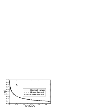
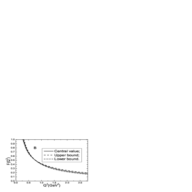
Figure 1: The $F_{\pi}^{p}(Q^{2})$(A) and $F_{\pi}^{q}(Q^{2})$(B) with the parameter $M^{2}=1\,\,\rm{GeV^{2}}$.

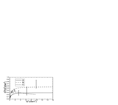
Figure 2: The numerical values of the form-factors $Q^{2}F_{\pi}^{p}(Q^{2})$(A) and $Q^{2}F_{\pi}^{q}(Q^{2})$(B) in comparison with the experimental data [3, 6, 7], line $C$ corresponds to the central values of $Q^{2}F_{\pi}(Q^{2})$ from the light-cone sum rules with the axial-vector current [14].

In the two sum rules in Eqs.(7-8), the dominant contributions come from the two-particle twist-3 light-cone distribution amplitudes $\varphi_{p}(u)$ and $\varphi_{\sigma}(u)$ due to the pseudoscalar current $J_{\pi}(x)$. The different values of the coefficients of the $\varphi_{\pi}(u)$ obtained in Ref.[43] and Ref.[49] respectively can lead to results of minor difference. If we choose the axial-vector current to interpolate the $\pi$ meson, the main contributions come from the twist-2 light-cone distribution amplitude $\varphi_{\pi}(u)$ [17, 18, 19, 20, 21]. The uncertainties concerning the denominator $\frac{1}{m_{u}+m_{d}}$ are canceled out with each other, see Eqs.(7-8), which result in small net uncertainties.

Taking into account all the uncertainties, finally we obtain the numerical values of the electromagnetic form-factors $F_{\pi}^{p}(Q^{2})$ and $F_{\pi}^{q}(Q^{2})$, which are shown in the Figs.1-2, at zero momentum transfer,

$$F_{\pi}^{p}(0) = 0.999\pm 0.001\,,$$

$$F_{\pi}^{q}(0) = 16.05\pm 1.82\,,$$ (10)

the parameters of the twist-2 light-cone distribution amplitude $\varphi_{\pi}(u)$ obtained in Ref.[49] can reduce the values of the form-factors $F_{\pi}^{p}(Q^{2})$ and $F_{\pi}^{q}(Q^{2})$ slightly, about $(1-2)\%$.

Comparing the experimental data (extrapolated to the limit $Q^{2}\rightarrow 0$, or the normalization condition $F_{\pi}(0)=1$) [1, 2, 3, 4, 5, 6, 7] and theoretical estimation with the vector meson dominance theory [50], our numerical value $F_{\pi}^{p}(0)=0.999\pm 0.001$ is excellent. The value $F_{\pi}^{q}(0)=16.05\pm 1.82$ is too large to make any reliable prediction, however, it is not un-expected. From the two sum rules, we can see that the terms of the $F_{\pi}^{q}(Q^{2})$ are companied with an extra factor $\frac{1}{u}$, for example,

$$F_{\pi}^{q}(Q^{2}) \propto \int_{\Delta}^{1}du\frac{\varphi_{p}(u)}{u}e^{-\frac{m_{q}^{2}+u(1-u)m_{\pi}^{2}-(1-u)q^{2}}{uM^{2}}}=\int_{\Delta}^{1}\frac{du}{u}e^{-\frac{m_{q}^{2}+u(1-u)m_{\pi}^{2}-(1-u)q^{2}}{uM^{2}}}\,,$$

$$F_{\pi}^{p}(Q^{2}) \propto \int_{\Delta}^{1}du\varphi_{p}(u)e^{-\frac{m_{q}^{2}+u(1-u)m_{\pi}^{2}-(1-u)q^{2}}{uM^{2}}}=\int_{\Delta}^{1}due^{-\frac{m_{q}^{2}+u(1-u)m_{\pi}^{2}-(1-u)q^{2}}{uM^{2}}}\,,$$

where we have taken the asymptotic distribution amplitude $\varphi_{p}(u)=1$. The value of the $F_{\pi}^{q}(Q^{2})$ is greatly enhanced in the region of small-$Q^{2}$ due to the extra $\frac{1}{u}$, in the limit $Q^{2}=0$, $\Delta\approx 0.00004$, the dominant contributions come from the end-point of the light-cone distribution amplitudes. We should introduce extra phenomenological form-factors (for example, the Sudakov factor [18, 19]) to suppress the contribution from the end-point. The value of the $F_{\pi}^{p}(Q^{2})$ is more reliable at small momentum transfers.

In the light-cone QCD sum rules, we carry out the operator product expansion near the light-cone $x^{2}\approx 0$, which corresponds to $Q^{2}\gg 0$ and $P^{2}\gg 0$, the two sum rules for the form-factors $F_{\pi}^{p}(Q^{2})$ and $F_{\pi}^{q}(Q^{2})$ are valid at large momentum transfers. We take the analytical expressions of the $F_{\pi}^{p}(Q^{2})$ and $F_{\pi}^{q}(Q^{2})$ in Eqs.(7-8) as some functions which model the electromagnetic form-factor $F_{\pi}(Q^{2})$ at large momentum transfers, then extrapolate the $F_{\pi}^{p}(Q^{2})$ and $F_{\pi}^{q}(Q^{2})$ to zero momentum transfer (or beyond zero momentum transfer) with analytical continuation in hope of obtaining some interesting results . It is obvious that the model functions $F_{\pi}^{p}(Q^{2})$ and $F_{\pi}^{q}(Q^{2})$ may have good or bad low-$Q^{2}$ behaviors, although they have solid theoretical foundation at large momentum transfers. We extrapolate the model functions tentatively to zero momentum transfer, systematic errors maybe very large and the results maybe unreliable. The predictions merely indicate the possible values of the light-cone QCD sum rules approach, they should be confronted with the experimental data or other theoretical approaches. The numerical results indicate that the small-$Q^{2}$ behavior of the $F_{\pi}^{p}(Q^{2})$ is better than that of the $F_{\pi}^{q}(Q^{2})$, so we take the value of the $F_{\pi}^{p}(Q^{2})$ at $Q^{2}<1\,\,\rm{GeV}^{2}$.

The electromagnetic form-factors $F_{\pi}^{p}(Q^{2})$ and $F_{\pi}^{q}(Q^{2})$ are complex functions of the input parameters, in principle, they can be expanded in terms of Taylor series of $\frac{1}{Q^{2}}$ for large-$Q^{2}$. At large momentum transfer, for example, $Q^{2}=(6-16)\,\,\rm{GeV}^{2}$, the central values of the two form-factors $F_{\pi}^{p}(Q^{2})$ and $F_{\pi}^{q}(Q^{2})$ can be fitted numerically as

$$F_{\pi}^{p}(Q^{2}) = \frac{0.285}{Q^{2}}\,,$$

$$F_{\pi}^{q}(Q^{2}) = \frac{0.554}{Q^{2}}\,,$$ (11)

which are comparable with the experimental data [1, 2, 3, 4, 5, 6, 7] and theoretical estimations, for examples, the light-cone QCD sum rules [12, 13, 14, 15], perturbative QCD [17, 18, 19, 20, 21]. In Fig.2, we plot the electromagnetic form-factor $Q^{2}F_{\pi}(Q^{2})$ comparing with the experimental data in Refs. [3, 6, 7] and prediction of the light-cone QCD sum rules with the axial-vector current in Ref.[14]. For more literatures, one can consult Ref.[53].

The large-$Q^{2}$ behavior $F_{\pi}(Q^{2})\sim\frac{1}{Q^{2}}$ is expected from the naive power counting rules [54, 55, 56]. At large-$Q^{2}$, the $i$-th term in the form-factors $F_{\pi}^{p}(Q^{2})$ and $F_{\pi}^{q}(Q^{2})$ respectively can be expanded as $\frac{A_{i}}{Q^{2}}+\frac{B_{i}}{Q^{4}}+\frac{C_{i}}{Q^{6}}+\cdots$, the terms proportional to $\frac{1}{Q^{2n}}$ with $n\geq 2$ are canceled out approximately with each other, i.e. $\sum B_{i}\approx 0$, $\sum C_{i}\approx 0$, $\cdots$. Finally we obtain $\sum A_{i}=0.285$ and $\sum A_{i}=0.554$ for the $F_{\pi}^{p}(Q^{2})$ and $F_{\pi}^{q}(Q^{2})$ respectively. Due to partial conservation of the axial-vector current, the axial-vector current has no-vanishing coupling with the $\pi$ meson, we can choose either the axial-vector current or the pseudoscalar current to interpolate the $\pi$ meson. They can lead to different sum rules, in the case of the axial-vector current, the soft contributions proportional to $\frac{1}{Q^{4}}$ manifest themselves at large-$Q^{2}$ [13, 14], see Fig.2, more experimental data are needed to select the pertinent sum rules.

In the limit of large-$Q^{2}$, $F_{\pi}(Q^{2})\sim\frac{1}{Q^{2}}$, which is consistent with the prediction of perturbative QCD theory, i.e. hard-gluon exchange between the $u$ and $d$ quarks dominates over Feynman mechanism.

4 Conclusion

In this article, we calculate the electromagnetic form-factor of the $\pi$ meson with the light-cone QCD sum rules. Our numerical value $F_{\pi}^{p}(0)=0.999\pm 0.001$ is in excellent agreement with the experimental data (extrapolated to the limit $Q^{2}\rightarrow 0$ or the normalization condition $F_{\pi}(0)=1$). For large momentum transfers, the values from the two sum rules are all comparable with the experimental data and theoretical estimations.

Appendix

The explicit expressions of the correlation functions,

$$\Pi_{p}^{u} = \frac{f_{\pi}m_{\pi}^{2}}{m_{u}+m_{d}}\int_{0}^{1}du\frac{u\varphi_{p}(u)}{m_{u}^{2}-(q+up)^{2}}-m_{u}f_{\pi}m_{\pi}^{2}\int_{0}^{1}du\int_{0}^{u}dt\frac{uB(t)}{\left[m_{u}^{2}-(q+up)^{2}\right]^{2}}$$ (12)

$$+\frac{1}{6}\frac{f_{\pi}m_{\pi}^{2}}{m_{u}+m_{d}}\int_{0}^{1}du\varphi_{\sigma}(u)\left\{\left[1-u\frac{d}{du}\right]\frac{1}{m_{u}^{2}-(q+up)^{2}}+\frac{2m_{u}^{2}}{\left[m_{u}^{2}-(q+up)^{2}\right]^{2}}\right\}$$

$$+m_{u}f_{\pi}\int_{0}^{1}du\left\{\frac{\varphi_{\pi}(u)}{m_{u}^{2}-(q+up)^{2}}-\frac{m_{\pi}^{2}m_{u}^{2}}{2}\frac{A(u)}{\left[m_{u}^{2}-(q+up)^{2}\right]^{3}}\right\}$$

$$-f_{3\pi}\int_{0}^{1}dv\int_{0}^{1}d\alpha_{g}\int_{0}^{1-\alpha_{g}}d\alpha_{u}\varphi_{3\pi}(\alpha_{d},\alpha_{g},\alpha_{u})$$

$$\left\{\frac{(1+2v)um_{\pi}^{2}}{\left[m_{u}^{2}-(q+up)^{2}\right]^{2}}-2(1-v)\frac{d}{du}\frac{1}{m_{u}^{2}-(q+up)^{2}}\right\}\mid_{u=(1-v)\alpha_{g}+\alpha_{u}}$$

$$+4m_{u}f_{\pi}m_{\pi}^{4}\int_{0}^{1}dvv\int_{0}^{1}d\alpha_{g}\int_{0}^{\alpha_{g}}d\beta\int_{0}^{1-\beta}d\alpha\frac{u\Phi(1-\alpha-\beta,\beta,\alpha)}{\left[m_{u}^{2}-(q+up)^{2}\right]^{3}}\mid_{1-v\alpha_{g}}$$

$$-4m_{u}f_{\pi}m_{\pi}^{4}\int_{0}^{1}dv\int_{0}^{1}d\alpha_{g}\int_{0}^{1-\alpha_{g}}d\alpha_{u}\int_{0}^{\alpha_{u}}d\alpha\frac{u\Phi(1-\alpha-\alpha_{g},\alpha_{g},\alpha)}{\left[m_{u}^{2}-(q+up)^{2}\right]^{3}}\mid_{u=(1-v)\alpha_{g}+\alpha_{u}}$$

$$+m_{u}f_{\pi}m_{\pi}^{2}\int_{0}^{1}dv\int_{0}^{1}d\alpha_{g}\int_{0}^{1-\alpha_{g}}d\alpha_{u}\frac{\Psi(\alpha_{d},\alpha_{g},\alpha_{u})}{\left[m_{u}^{2}-(q+up)^{2}\right]^{2}}\mid_{u=(1-v)\alpha_{g}+\alpha_{u}}\,,$$

$$\Pi_{p}^{d} = -\frac{f_{\pi}m_{\pi}^{2}}{m_{u}+m_{d}}\int_{0}^{1}du\frac{u\varphi_{p}(u)}{m_{d}^{2}-(q+up)^{2}}+m_{d}f_{\pi}m_{\pi}^{2}\int_{0}^{1}du\int_{0}^{u}dt\frac{uB(t)}{\left[m_{d}^{2}-(q+up)^{2}\right]^{2}}$$ (13)

$$-\frac{1}{6}\frac{f_{\pi}m_{\pi}^{2}}{m_{u}+m_{d}}\int_{0}^{1}du\varphi_{\sigma}(u)\left\{\left[1-u\frac{d}{du}\right]\frac{1}{m_{d}^{2}-(q+up)^{2}}+\frac{2m_{d}^{2}}{\left[m_{d}^{2}-(q+up)^{2}\right]^{2}}\right\}$$

$$-m_{d}f_{\pi}\int_{0}^{1}du\left\{\frac{\varphi_{\pi}(u)}{m_{d}^{2}-(q+up)^{2}}-\frac{m_{\pi}^{2}m_{d}^{2}}{2}\frac{A(u)}{\left[m_{d}^{2}-(q+up)^{2}\right]^{3}}\right\}$$

$$+f_{3\pi}\int_{0}^{1}dv\int_{0}^{1}d\alpha_{g}\int_{0}^{1-\alpha_{g}}d\alpha_{d}\varphi_{3\pi}(\alpha_{d},\alpha_{g},\alpha_{u})$$

$$\left\{\frac{(1+2v)um_{\pi}^{2}}{\left[m_{d}^{2}-(q+up)^{2}\right]^{2}}-2(1-v)\frac{d}{du}\frac{1}{m_{d}^{2}-(q+up)^{2}}\right\}\mid_{u=(1-v)\alpha_{g}+\alpha_{d}}$$

$$+4m_{d}f_{\pi}m_{\pi}^{4}\int_{0}^{1}dvv\int_{0}^{1}d\alpha_{g}\int_{0}^{\alpha_{g}}d\beta\int_{0}^{1-\beta}d\alpha\frac{u\widetilde{\Phi}(\alpha,\beta,1-\alpha-\beta)}{\left[m_{d}^{2}-(q+up)^{2}\right]^{3}}\mid_{1-v\alpha_{g}}$$

$$-4m_{d}f_{\pi}m_{\pi}^{4}\int_{0}^{1}dv\int_{0}^{1}d\alpha_{g}\int_{0}^{1-\alpha_{g}}d\alpha_{d}\int_{0}^{\alpha_{d}}d\alpha\frac{u\widetilde{\Phi}(\alpha,\alpha_{g},1-\alpha-\alpha_{g})}{\left[m_{d}^{2}-(q+up)^{2}\right]^{3}}\mid_{u=(1-v)\alpha_{g}+\alpha_{d}}$$

$$+m_{d}f_{\pi}m_{\pi}^{2}\int_{0}^{1}dv\int_{0}^{1}d\alpha_{g}\int_{0}^{1-\alpha_{g}}d\alpha_{d}\frac{\widetilde{\Psi}(\alpha_{d},\alpha_{g},\alpha_{u})}{\left[m_{d}^{2}-(q+up)^{2}\right]^{2}}\mid_{u=(1-v)\alpha_{g}+\alpha_{d}}\,,$$

$$\Pi_{q}^{u} = \frac{f_{\pi}m_{\pi}^{2}}{m_{u}+m_{d}}\int_{0}^{1}du\frac{\varphi_{p}(u)}{m_{u}^{2}-(q+up)^{2}}-m_{u}f_{\pi}m_{\pi}^{2}\int_{0}^{1}du\int_{0}^{u}dt\frac{B(t)}{\left[m_{u}^{2}-(q+up)^{2}\right]^{2}}$$

$$-\frac{1}{6}\frac{f_{\pi}m_{\pi}^{2}}{m_{u}+m_{d}}\int_{0}^{1}du\varphi_{\sigma}(u)\frac{d}{du}\frac{1}{m_{u}^{2}-(q+up)^{2}}$$

$$-f_{3\pi}m_{\pi}^{2}\int_{0}^{1}dv\int_{0}^{1}d\alpha_{g}\int_{0}^{1-\alpha_{g}}d\alpha_{u}\varphi_{3\pi}(\alpha_{d},\alpha_{g},\alpha_{u})\frac{1+2v}{\left[m_{u}^{2}-(q+up)^{2}\right]^{2}}\mid_{u=(1-v)\alpha_{g}+\alpha_{u}}$$

$$+4m_{u}f_{\pi}m_{\pi}^{4}\int_{0}^{1}dvv\int_{0}^{1}d\alpha_{g}\int_{0}^{\alpha_{g}}d\beta\int_{0}^{1-\beta}d\alpha\frac{\Phi(1-\alpha-\beta,\beta,\alpha)}{\left[m_{u}^{2}-(q+up)^{2}\right]^{3}}\mid_{1-v\alpha_{g}}$$

$$-4m_{u}f_{\pi}m_{\pi}^{4}\int_{0}^{1}dv\int_{0}^{1}d\alpha_{g}\int_{0}^{1-\alpha_{g}}d\alpha_{u}\int_{0}^{\alpha_{u}}d\alpha\frac{\Phi(1-\alpha-\alpha_{g},\alpha_{g},\alpha)}{\left[m_{u}^{2}-(q+up)^{2}\right]^{3}}\mid_{u=(1-v)\alpha_{g}+\alpha_{u}}\,,$$

$$\Pi_{q}^{d} = -\frac{f_{\pi}m_{\pi}^{2}}{m_{u}+m_{d}}\int_{0}^{1}du\frac{\varphi_{p}(u)}{m_{d}^{2}-(q+up)^{2}}+m_{d}f_{\pi}m_{\pi}^{2}\int_{0}^{1}du\int_{0}^{u}dt\frac{B(t)}{\left[m_{d}^{2}-(q+up)^{2}\right]^{2}}$$

$$+\frac{1}{6}\frac{f_{\pi}m_{\pi}^{2}}{m_{u}+m_{d}}\int_{0}^{1}du\varphi_{\sigma}(u)\frac{d}{du}\frac{1}{m_{d}^{2}-(q+up)^{2}}$$

$$+f_{3\pi}m_{\pi}^{2}\int_{0}^{1}dv\int_{0}^{1}d\alpha_{g}\int_{0}^{1-\alpha_{g}}d\alpha_{d}\varphi_{3\pi}(\alpha_{d},\alpha_{g},\alpha_{u})\frac{1+2v}{\left[m_{d}^{2}-(q+up)^{2}\right]^{2}}\mid_{u=(1-v)\alpha_{g}+\alpha_{d}}$$

$$+4m_{d}f_{\pi}m_{\pi}^{4}\int_{0}^{1}dvv\int_{0}^{1}d\alpha_{g}\int_{0}^{\alpha_{g}}d\beta\int_{0}^{1-\beta}d\alpha\frac{\widetilde{\Phi}(\alpha,\beta,1-\alpha-\beta)}{\left[m_{d}^{2}-(q+up)^{2}\right]^{3}}\mid_{1-v\alpha_{g}}$$

$$-4m_{d}f_{\pi}m_{\pi}^{4}\int_{0}^{1}dv\int_{0}^{1}d\alpha_{g}\int_{0}^{1-\alpha_{g}}d\alpha_{d}\int_{0}^{\alpha_{d}}d\alpha\frac{\widetilde{\Phi}(\alpha,\alpha_{g},1-\alpha-\alpha_{g})}{\left[m_{d}^{2}-(q+up)^{2}\right]^{3}}\mid_{u=(1-v)\alpha_{g}+\alpha_{d}}\,,$$

where

$$\Phi = A_{\parallel}+A_{\perp}-V_{\perp}-V_{\parallel}\,,$$

$$\widetilde{\Phi} = A_{\parallel}+A_{\perp}+V_{\perp}+V_{\parallel}\,,$$

$$\Psi = 2A_{\perp}-2V_{\perp}-A_{\parallel}+V_{\parallel}\,,$$

$$\widetilde{\Psi} = 2A_{\perp}+2V_{\perp}-A_{\parallel}-V_{\parallel}\,.$$

The light-cone distribution amplitudes of the $\pi$ meson are defined as

$$\langle 0|{\bar{u}}(0)\gamma_{\mu}\gamma_{5}d(x)|\pi(p)\rangle = if_{\pi}p_{\mu}\int_{0}^{1}due^{-iup\cdot x}\left\{\varphi_{\pi}(u)+\frac{m_{\pi}^{2}x^{2}}{16}A(u)\right\}$$

$$+if_{\pi}m_{\pi}^{2}\frac{x_{\mu}}{2p\cdot x}\int_{0}^{1}due^{-iup\cdot x}B(u)\,,$$

$$\langle 0|{\bar{u}}(0)i\gamma_{5}d(x)|\pi(p)\rangle = \frac{f_{\pi}m_{\pi}^{2}}{m_{u}+m_{d}}\int_{0}^{1}due^{-iup\cdot x}\varphi_{p}(u)\,,$$

$$\langle 0|{\bar{u}}(0)\sigma_{\mu\nu}\gamma_{5}d(x)|\pi(p)\rangle = i(p_{\mu}x_{\nu}-p_{\nu}x_{\mu})\frac{f_{\pi}m_{\pi}^{2}}{6(m_{u}+m_{d})}\int_{0}^{1}due^{-iup\cdot x}\varphi_{\sigma}(u)\,,$$

$$\langle 0|{\bar{u}}(0)\sigma_{\alpha\beta}\gamma_{5}g_{s}G_{\mu\nu}(vx)d(x)|\pi(p)\rangle = f_{3\pi}\left\{(p_{\mu}p_{\alpha}g^{\bot}_{\nu\beta}-p_{\nu}p_{\alpha}g^{\bot}_{\mu\beta})-(p_{\mu}p_{\beta}g^{\bot}_{\nu\alpha}\right.$$

$$\left.-p_{\nu}p_{\beta}g^{\bot}_{\mu\alpha})\right\}\int{\cal D}\alpha_{i}\varphi_{3\pi}(\alpha_{i})e^{-ip\cdot x(\alpha_{d}+v\alpha_{g})}\,,$$

$$\langle 0|{\bar{u}}(0)\gamma_{\mu}\gamma_{5}g_{s}G_{\alpha\beta}(vx)d(x)|\pi(p)\rangle = p_{\mu}\frac{p_{\alpha}x_{\beta}-p_{\beta}x_{\alpha}}{p\cdot x}f_{\pi}m_{\pi}^{2}$$

$$\int{\cal D}\alpha_{i}A_{\parallel}(\alpha_{i})e^{-ip\cdot x(\alpha_{d}+v\alpha_{g})}$$

$$+f_{\pi}m_{\pi}^{2}(p_{\beta}g_{\alpha\mu}-p_{\alpha}g_{\beta\mu})$$

$$\int{\cal D}\alpha_{i}A_{\perp}(\alpha_{i})e^{-ip\cdot x(\alpha_{d}+v\alpha_{g})}\,,$$

$$\langle 0|{\bar{u}}(0)\gamma_{\mu}g_{s}\tilde{G}_{\alpha\beta}(vx)d(x)|\pi(p)\rangle = p_{\mu}\frac{p_{\alpha}x_{\beta}-p_{\beta}x_{\alpha}}{p\cdot x}f_{\pi}m_{\pi}^{2}$$ (16)

$$\int{\cal D}\alpha_{i}V_{\parallel}(\alpha_{i})e^{-ip\cdot x(\alpha_{d}+v\alpha_{g})}$$

$$+f_{\pi}m_{\pi}^{2}(p_{\beta}g_{\alpha\mu}-p_{\alpha}g_{\beta\mu})$$

$$\int{\cal D}\alpha_{i}V_{\perp}(\alpha_{i})e^{-ip\cdot x(\alpha_{d}+v\alpha_{g})}\,,$$

where $\tilde{G}_{\alpha\beta}={1\over 2}\epsilon_{\alpha\beta\mu\nu}G^{\mu\nu}$ and ${\cal{D}}\alpha_{i}=d\alpha_{1}d\alpha_{2}d\alpha_{3}\delta(1-\alpha_{1}-\alpha_{2}-\alpha_{3})$.

The light-cone distribution amplitudes are parameterized as

$$\varphi_{\pi}(u) = 6u(1-u)\left\{1+a_{1}C^{\frac{3}{2}}_{1}(2u-1)+a_{2}C^{\frac{3}{2}}_{2}(2u-1)+a_{4}C^{\frac{3}{2}}_{4}(2u-1)\right\}\,,$$

$$\varphi_{p}(u) = 1+\left\{30\eta_{3}-\frac{5}{2}\rho^{2}\right\}C_{2}^{\frac{1}{2}}(2u-1)$$

$$+\left\{-3\eta_{3}\omega_{3}-\frac{27}{20}\rho^{2}-\frac{81}{10}\rho^{2}a_{2}\right\}C_{4}^{\frac{1}{2}}(2u-1)\,,$$

$$\varphi_{\sigma}(u) = 6u(1-u)\left\{1+\left[5\eta_{3}-\frac{1}{2}\eta_{3}\omega_{3}-\frac{7}{20}\rho^{2}-\frac{3}{5}\rho^{2}a_{2}\right]C_{2}^{\frac{3}{2}}(2u-1)\right\}\,,$$

$$\varphi_{3\pi}(\alpha_{i}) = 360\alpha_{u}\alpha_{d}\alpha_{g}^{2}\left\{1+\lambda_{3}(\alpha_{u}-\alpha_{d})+\omega_{3}\frac{1}{2}(7\alpha_{g}-3)\right\}\,,$$

$$V_{\parallel}(\alpha_{i}) = 120\alpha_{u}\alpha_{d}\alpha_{g}\left(v_{00}+v_{10}(3\alpha_{g}-1)\right)\,,$$

$$A_{\parallel}(\alpha_{i}) = 120\alpha_{u}\alpha_{d}\alpha_{g}a_{10}(\alpha_{d}-\alpha_{u})\,,$$

$$V_{\perp}(\alpha_{i}) = -30\alpha_{g}^{2}\left\{h_{00}(1-\alpha_{g})+h_{01}\left[\alpha_{g}(1-\alpha_{g})-6\alpha_{u}\alpha_{d}\right]\right.$$

$$\left.+h_{10}\left[\alpha_{g}(1-\alpha_{g})-\frac{3}{2}\left(\alpha_{u}^{2}+\alpha_{d}^{2}\right)\right]\right\}\,,$$

$$A_{\perp}(\alpha_{i}) = 30\alpha_{g}^{2}(\alpha_{u}-\alpha_{d})\left\{h_{00}+h_{01}\alpha_{g}+\frac{1}{2}h_{10}(5\alpha_{g}-3)\right\},$$

$$A(u) = 6u(1-u)\left\{\frac{16}{15}+\frac{24}{35}a_{2}+20\eta_{3}+\frac{20}{9}\eta_{4}\right.$$

$$+\left[-\frac{1}{15}+\frac{1}{16}-\frac{7}{27}\eta_{3}\omega_{3}-\frac{10}{27}\eta_{4}\right]C^{\frac{3}{2}}_{2}(2u-1)$$

$$\left.+\left[-\frac{11}{210}a_{2}-\frac{4}{135}\eta_{3}\omega_{3}\right]C^{\frac{3}{2}}_{4}(2u-1)\right\}+\left\{-\frac{18}{5}a_{2}+21\eta_{4}\omega_{4}\right\}$$

$$\left\{2u^{3}(10-15u+6u^{2})\log u+2\bar{u}^{3}(10-15\bar{u}+6\bar{u}^{2})\log\bar{u}\right.$$

$$\left.+u\bar{u}(2+13u\bar{u})\right\}\,,$$

$$g_{\pi}(u) = 1+g_{2}C^{\frac{1}{2}}_{2}(2u-1)+g_{4}C^{\frac{1}{2}}_{4}(2u-1)\,,$$

$$B(u) = g_{\pi}(u)-\varphi_{\pi}(u)\,,$$ (17)

where

$$h_{00} = v_{00}=-\frac{\eta_{4}}{3}\,,$$

$$a_{10} = \frac{21}{8}\eta_{4}\omega_{4}-\frac{9}{20}a_{2}\,,$$

$$v_{10} = \frac{21}{8}\eta_{4}\omega_{4}\,,$$

$$h_{01} = \frac{7}{4}\eta_{4}\omega_{4}-\frac{3}{20}a_{2}\,,$$

$$h_{10} = \frac{7}{2}\eta_{4}\omega_{4}+\frac{3}{20}a_{2}\,,$$

$$g_{2} = 1+\frac{18}{7}a_{2}+60\eta_{3}+\frac{20}{3}\eta_{4}\,,$$

$$g_{4} = -\frac{9}{28}a_{2}-6\eta_{3}\omega_{3}\,,$$ (18)

$C_{2}^{\frac{1}{2}}(\xi)$, $C_{4}^{\frac{1}{2}}(\xi)$ , $C_{2}^{\frac{3}{2}}(\xi)$ and $C_{4}^{\frac{3}{2}}(\xi)$ are Gegenbauer polynomials, $\eta_{3}=\frac{f_{3\pi}}{f_{\pi}}\frac{m_{u}+m_{d}}{m_{\pi}^{2}}$ and $\rho^{2}={(m_{u}+m_{d})^{2}\over m_{\pi}^{2}}$ [30, 31, 32, 33, 34, 39, 40, 41, 42, 43].

References

- [1] C. J. Bebek et al, Phys. Rev. D13 (1976) 25.
- [2] G. T. Adylov et al, Nucl. Phys. B128 (1977) 461.
- [3] C. J. Bebek et al, Phys. Rev. D17 (1978) 1693.
- [4] E. B. Dally et al, Phys. Rev. Lett. 48 (1982) 375.
- [5] S. R. Amendolia et al, Phys. Lett. B146 (1984) 116.
- [6] S. R. Amendolia et al, Nucl. Phys. B277 (1986) 168.
- [7] J. Volmer et al, Phys. Rev. Lett. 86 (2001) 1713.
- [8] V. A. Nesterenko and A. V. Radyushkin, Phys. Lett. B115 (1982) 410.
- [9] B. L. Ioffe and A. V. Smilga, Phys. Lett. B114 (1982) 353.
- [10] A. P. Bakulev and A. V. Radyushkin, Phys. Lett. B271 (1991) 223.
- [11] A. V. Radyushkin and R. T. Ruskov, Nucl. Phys. B481 (1996) 625.
- [12] V. M. Braun and I. E. Halperin, Phys. Lett. B328 (1994) 457.
- [13] V. M. Braun, A. Khodjamirian and M. Maul, Phys. Rev. D61 (2000) 073004.
- [14] J. Bijnens and A. Khodjamirian, Eur. Phys. J. C26 (2002) 67.
- [15] S. S. Agaev, Phys. Rev. D72 (2005) 074020.
- [16] A. V. Radyushkin, hep-ph/0410276.
- [17] G. P. Lepage and S. J. Brodsky, Phys. Rev. D22 (1980) 2157.
- [18] H. n. Li and G. Sterman, Nucl. Phys. B381 (1992) 129.
- [19] R. Jakob and P. Kroll, Phys. Lett. B315 (1993) 463.
- [20] T. Huang, X.-G. Wu and X.-H. Wu, Phys. Rev. D70 (2004) 053007.
- [21] A. P. Bakulev, K. Passek-Kumericki, W. Schroers and N. G. Stefanis, Phys. Rev. D70 (2004) 033014 .
- [22] P. Maris and P. C. Tandy, Phys. Rev. C62 (2000) 055204.
- [23] Z. G. Wang, S. L. Wan and K. L. Wang, Commun. Theor. Phys. 35 (2001) 697.
- [24] P. Maris and P. C. Tandy, Phys. Rev. C65 (2002) 045211.
- [25] Z. G. Wang, S. L. Wan and W. M. Yang, Phys. Rev. D73 (2006) 094011.
- [26] Z. G. Wang, S. L. Wan and W. M. Yang, Eur. Phys. J. C47 (2006) 375.
- [27] Z. G. Wang, J. Phys. G34 (2007) 493.
- [28] Z. G. Wang and S. L. Wan, Eur. Phys. J. C50 (2007) 781.
- [29] Z. G. Wang, J. Phys. G34 (2007) 2183.
- [30] I. I. Balitsky, V. M. Braun and A. V. Kolesnichenko, Nucl. Phys. B312 (1989) 509.
- [31] V. L. Chernyak and I. R. Zhitnitsky, Nucl. Phys. B345 (1990) 137.
- [32] V. L. Chernyak and A. R. Zhitnitsky, Phys. Rept. 112 (1984) 173.
- [33] V. M. Braun and I. E. Filyanov, Z. Phys. C44 (1989) 157.
- [34] V. M. Braun and I. E. Filyanov, Z. Phys. C48 (1990) 239.
- [35] V. M. Braun, hep-ph/9801222.
- [36] P. Colangelo and A. Khodjamirian, hep-ph/0010175.
- [37] M. A. Shifman, A. I. Vainshtein and V. I. Zakharov, Nucl. Phys. B147 (1979) 385, 448.
- [38] L. J. Reinders, H. Rubinstein and S. Yazaki, Phys. Rept. 127 (1985) 1.
- [39] V. M. Belyaev, V. M. Braun, A. Khodjamirian and R. Rückl, Phys. Rev. D51 (1995) 6177.
- [40] P. Ball, JHEP 9901 (1999) 010.
- [41] P. Ball and R. Zwicky, Phys. Lett. B633 (2006) 289.
- [42] P. Ball and R. Zwicky, JHEP 0602 (2006) 034.
- [43] P. Ball, V. M. Braun and A. Lenz, JHEP 0605 (2006) 004.
- [44] A. Schmedding and O. I. Yakovlev, Phys. Rev. D62 (2000) 116002.
- [45] A. P. Bakulev, S. V. Mikhailov and N. G. Stefanis, Phys. Lett. B508 (2001) 279.
- [46] A. P. Bakulev, S. V. Mikhailov and N. G. Stefanis, Phys. Rev. D67 (2003) 074012.
- [47] A. P. Bakulev, S. V. Mikhailov and N. G. Stefanis, Phys. Lett. B578 (2004) 91.
- [48] A. P. Bakulev and A. V. Pimikov, Acta. Phys. Polon. B37 (2006) 3627.
- [49] A. P. Bakulev, hep-ph/0611139.
- [50] J. J. Sakurai, Annals Phys. 11 (1960) 1.
- [51] S. J. Brodsky and G. P. Lepage, Phys. Rev. D24 (1981) 1808.
- [52] J. Gronberg et al, Phys. Rev. D57 (1998) 33; and references therein.
- [53] P. Zweber, hep-ex/0605026; and the references therein.
- [54] S. J. Brodsky and G. R. Farrar, Phys. Rev. Lett. 31 (1973) 1153.
- [55] S. J. Brodsky and G. R. Farrar, Phys. Rev. D11 (1975) 1309.
- [56] D. W. Sivers, S. J. Brodsky and R. Blankenbecler, Phys. Rept. 23 (1976) 1.