Finite temperature behavior of strongly disordered quantum magnets coupled to a dissipative bath

Abstract

We study the effect of dissipation on the infinite randomness fixed point and the Griffiths-McCoy singularities of random transverse Ising systems in chains, ladders and in two-dimensions. A strong disorder renormalization group scheme is presented that allows the computation of the finite temperature behavior of the magnetic susceptibility and the spin specific heat. In the case of Ohmic dissipation the susceptibility displays a crossover from Griffiths-McCoy behavior (with a continuously varying dynamical exponent) to classical Curie behavior at some temperature $T^{*}$. The specific heat displays Griffiths-McCoy singularities over the whole temperature range. For super-Ohmic dissipation we find an infinite randomness fixed point within the same universality class as the transverse Ising system without dissipation. In this case the phase diagram and the parameter dependence of the dynamical exponent in the Griffiths-McCoy phase can be determined analytically.

1 Introduction

The interplay between quantum fluctuations and quenched disorder in the form of an extensive amount impurities or other random spatial inhomogeneities can lead to a new class of quantum phase transitions, governed by an infinite randomness fixed point (IRFP) as established for transverse Ising models [1] and many other disordered quantum systems (for an overview see [3]). Besides unusual scaling laws at the transition the IRFP is characterized by a whole parameter range around the transition, in which physical observables display singular and even divergent behavior in spite of a finite spatial correlation length. This is the manifestation of Griffiths-McCoy singularities or quantum Griffiths behavior [4, 6, 8, 10, 12]. They have their origin in rare regions of strongly coupled spins (or other quantum mechanical degrees of freedoms) that tend to order locally and thus produce a strong response to small external fields, long relaxation (or tunneling) times and small excitation energies.

If the underlying quantum phase transition is governed by an infinite randomness fixed point the statistics of these rare events leads to a power law divergence of the susceptibility in a region around the quantum critical point with a continuously varying exponent. This dynamical exponent determines all singularities in the Griffiths-McCoy phase. Continuously varying exponents, interrelated in a specific way for different physical observables, were observed in many heavy-fermion materials, and it was argued that this is a manifestation of Griffiths-McCoy behavior due to an underlying IRFP [14, 16]. In essence these systems form local moments that interact via long-range RKKY interaction and have a strong Ising anisotropy, such that an effective model describing these degrees of freedom and their interaction is a random transverse Ising system.

Later it was argued that due to the interaction via band electrons the effective spin degrees of freedom are strongly coupled to a dissipative Ohmic bath [17, 19]. From this point of view the rare regions should be described by spin-boson systems, which are known to behave classically for sufficiently strong coupling to the dissipative bath [21], which would destroy the expected Griffiths-McCoy singularities.

Since in the presence of dissipation rare regions can undergo phase transitions and freeze independently from one another (like in the McCoy-Wu model in the mean-field approximation [22]), the global phase transition of the system is destroyed by smearing because different spatial parts of the system order at different values of the control parameter [23, 24].

Recently we analyzed the random transverse Ising chain coupled to a Ohmic dissipative bath with a strong disorder renormalization group (SDRG) scheme and could demonstrate that the transition is indeed smeared, but argued that Griffiths-McCoy singularities are still observable, at least down to very low temperatures also in the presence of dissipation [25]. This was done by analyzing the gap and cluster distribution. In this paper we continue and extend this SDRG study by a) analyzing the low temperature behavior of the magnetic susceptibility and the spin specific heat in the case of Ohmic dissipation, where we will argue that Griffiths-McCoy singularities are visible at all temperatures in the specific heat and above a (small) crossover temperature in the susceptibility; b) considering in addition to chains also ladders and two-dimensional systems, where we obtain similar results as for the chain; and c) applying the SDRG also to super-Ohmic dissipation, where we find a quantum phase transition belonging to the same IRFP universality class as the system without dissipation and compute analytically the phase diagram and dynamical exponent in the Griffiths-McCoy phase.

The system that we study is the random transverse Ising model where each spin is coupled to a dissipative bath of harmonic oscillators, i.e. ferromagnetically coupled spin-boson systems [21]. It is defined on $d$-dimensional square lattice of linear size $L$ with periodic boundary conditions (pbc) and described by the Hamiltonian

$$H=-\sum_{\langle i,j\rangle}J_{ij}\sigma_{i}^{z}\sigma_{j}^{z}-\sum_{i}\biggl{[}h_{i}\sigma_{i}^{x}+\sum_{k}\Bigl{(}C_{k,i}\hat{x}_{k,i}\sigma_{i}^{z}+\frac{\hat{p}_{k,i}^{2}}{2}+\omega_{k,i}^{2}\frac{\hat{x}_{k,i}^{2}}{2}\Bigr{)}\biggr{]}\;,$$ (1)

where $\sigma_{i}^{x,z}$ are Pauli matrices and the masses of the oscillators are set to one. The quenched random bonds $J_{i}$ (respectively random transverse field $h_{i}$) are uniformly distributed between $0$ and $J_{0}$ (respectively between $0$ and $h_{0}$). The properties of the bath are specified by its spectral function ${\cal J}_{i}(\omega)$

$${\cal J}_{i}(\omega)=\frac{\pi}{2}\sum_{k}\frac{C_{k,i}^{2}}{\omega_{k,i}}\delta(\omega-\omega_{k,i})=\frac{\pi}{2}\alpha_{i}\Omega_{i}^{1-s}\omega^{s}\theta(\Omega_{i}-\omega)\;,$$ (2)

where $\Omega_{i}$ is a cutoff frequency and $\theta(x)$ the Heaviside function such that $\theta(x)=1$ if $x>0$ and $\theta(x)=0$ if $x<0$. The case $s=1$ is known as Ohmic dissipation although $s>1$ (respectively $s<1$) corresponds to a super-ohmic (respectively sub-ohmic) dissipation. Initially the spin-bath couplings and cut-off frequencies are site-independent, i.e. $\alpha_{i}=\alpha$ and $\Omega_{i}=\Omega$, but both become site-dependent under renormalization.

2 Real space renormalization.

2.1 Decimation procedure.

In this section, we derive in detail the real space renormalization scheme to study dissipative random transverse Ising model as in Eq. (1). For simplicity, we present the calculation in dimension $d=1$ (extensions to higher dimensions are discussed below) and focus on the random transverse Ising chain (RTFIC):

$$H_{1d}=\sum^{L}_{i=1}\biggl{[}-J_{i}\sigma_{i}^{z}\sigma_{i+1}^{z}-h_{i}\sigma_{i}^{x}+\sum_{k}\Bigl{(}C_{k,i}\hat{x}_{k,i}\sigma_{i}^{z}+\frac{\hat{p}_{k,i}^{2}}{2}+\omega_{k,i}^{2}\frac{\hat{x}_{k,i}^{2}}{2}\Bigr{)}\biggr{]}\;.$$ (3)

To characterize the ground state properties of this system (1), we follow the idea of a real space renormalization group (RG) procedure introduced in Ref. [26] and pushed further in the context of the RTFIC without dissipation in Ref. [4]. The strategy is to find the largest coupling in the chain, either a transverse field or a bond, compute the ground state of the associated part of the Hamiltonian and treat the remaining couplings in perturbation theory. The bath degrees of freedom are dealt with in the spirit of the “adiabatic renormalization” introduced in the context of the (single) spin-boson (SB) model [21], where it describes accurately its critical behavior [28].

2.1.1 When the largest coupling is a bond.

Suppose that the largest coupling in the chain is a bond, say $J_{2}$. The associated part $H_{2}$ of the full Hamiltonian $H_{1d}$ in Eq. (3) is

$$H_{2}= H_{2}^{(0)} +V$$

$$H_{2}^{(0)} =-J_{2}\sigma_{2}^{z}\sigma_{3}^{z}+\sum_{i=2,3}\sum_{k}\Bigl{(}C_{k,i}\hat{x}_{k,i}\sigma_{i}^{z}+\frac{\hat{p}_{k,i}^{2}}{2}+\omega_{k,i}^{2}\frac{\hat{x}_{k,i}^{2}}{2}\Bigr{)}$$

$$V =-h_{2}\sigma_{2}^{x}-h_{3}\sigma_{3}^{x}\;.$$

Let us first focus on $H_{2}^{(0)}$ in Eq. (2.1.1) and first introduce the notation for the spin part $|{\mathbf{S}}\rangle\equiv|S_{2},S_{3}\rangle$, with $S_{i}=\pm 1$ such that $\sigma_{i}^{z}|{\mathbf{S}}\rangle=S_{i}|{\mathbf{S}}\rangle$ for $i=2,3$. Considering now the two baths on site $i=2,3$ respectively, they are composed of a set of harmonic oscillators which are labeled by an integer $k$ (which formally runs from $0$ to $\infty$) and by $i=2,3$. We denote by $|n_{k,i}\rangle$ the eigenvalues of these harmonic oscillators such that

$$\left(\frac{\hat{p}_{k,i}^{2}}{2}+\omega_{k,i}^{2}\frac{\hat{x}_{k,i}^{2}}{2}\right)|n_{k,i}\rangle=(n_{k,i}+\frac{1}{2})\omega_{k,i}|n_{k,i}\rangle\;.$$ (5)

In the absence of the coupling between the spins and the bath, $H_{2}^{(0)}$ can be straightforwardly diagonalized by tensorial products of $|{\mathbf{S}}\rangle$ and $|n_{k,i}\rangle$. The corresponding eigenvalues are simply the sum of the eigenvalues of the individual Hamiltonians in Eq. (2.1.1) without the last term of interaction. The coupling between the spins and the baths does not change these eigenvalues (up to a global shift) and only affects the eigenstates. We introduce the shifted "eigenvectors"

$$|n_{k,j}^{\pm}\rangle=\exp{\left(\pm i\frac{C_{k,j}}{\omega_{k,j}^{2}}\hat{p}_{k,j}\right)}|n_{k,j}\rangle\quad,\quad j=2,3\;,$$ (6)

from which we can construct the eigenvectors of $H_{2}^{(0)}$, including the interaction between the baths and the spins as

$$|{\mathbf{S}},{\mathbf{n}}\rangle = |S_{2},S_{3}\rangle\otimes|{\mathfrak{n}}_{2}^{S_{2}}\rangle\otimes|{\mathfrak{n}}_{3}^{S_{3}}\rangle$$

$$|{\mathfrak{n}}_{i}^{S_{i}}\rangle = \bigotimes_{k}|n_{k,i}^{S_{i}}\rangle\;.$$ (7)

The eigenvalues of $H_{2}^{(0)}$ are given by

$$H_{2}^{(0)}|{\mathbf{S}},{\mathbf{n}}\rangle = E^{(0)}_{{\mathbf{S}},{\mathbf{n}}}|{\mathbf{S}},{\mathbf{n}}\rangle\;,$$

$$E^{(0)}_{{\mathbf{S}},{\mathbf{n}}} = -J_{2}S_{2}S_{3}+\sum_{i=2,3}\sum_{k}\biggl{[}\Bigl{(}n_{k,i}+\frac{1}{2}\Bigr{)}\omega_{k,i}-\frac{1}{2}\frac{C_{k,i}^{2}}{\omega_{k,i}^{2}}\biggr{]}\;.$$ (8)

Each level is thus a priori degenerated twice (except accidental degeneracy) and in the limit of large coupling $J_{2}$ we first restrict ourselves to the lowest energy levels, such that $S_{2}S_{3}=+1$. Performing perturbation theory in $V$, one obtains that the first order corrections vanish. To second order in $V$, one has to diagonalize the $2\times 2$ matrix $V^{(2)}$ in the eigensubspace associated to the zeroth order eigenvalue $E^{(0)}_{{\mathbf{S}},{\mathbf{n}}}$ with $S_{2}S_{3}=+1$ which is formally given by

$$V^{(2)}=\sum_{{\mathbf{S}^{\prime}},{\mathbf{n}^{\prime}},E_{{\mathbf{S}^{\prime}},{\mathbf{n}^{\prime}}}\neq E_{{\mathbf{S}},{\mathbf{n}}}}\frac{V|{\mathbf{S}}^{\prime},{\mathbf{n}}^{\prime}\rangle\langle{\mathbf{S}}^{\prime},{\mathbf{n}}^{\prime}|V}{E^{(0)}_{{\mathbf{S}},{\mathbf{n}}}-E^{(0)}_{{\mathbf{S}^{\prime}},{\mathbf{n}}^{\prime}}}\;.$$ (9)

One obtains from (9) the diagonal elements

$$V^{(2)}_{11}=V^{(2)}_{22} =h_{2}^{2}\sum_{{\mathfrak{n}}^{\prime}_{2}}\frac{|\langle{\mathfrak{n}}_{2}^{+}|{{\mathfrak{n}}^{\prime}_{2}}^{-}\rangle|^{2}}{-2J_{2}+\sum_{k}(n_{k,2}-n^{\prime}_{k,2})\omega_{k,2}}$$ (10)

$$+h_{3}^{2}\sum_{{\mathfrak{n}}^{\prime}_{3}}\frac{|\langle{\mathfrak{n}}_{3}^{+}|{{\mathfrak{n}}^{\prime}_{3}}^{-}\rangle|^{2}}{-2J_{2}+\sum_{k}(n_{k,3}-n^{\prime}_{k,3})\omega_{k,3}}\;,$$

and the off-diagonal elements

$$V_{12}^{(2)}=V_{21}^{(2)}=-\frac{h_{2}h_{3}}{J_{2}}\langle{\mathfrak{n}}_{2}^{-}|{\mathfrak{n}}_{2}^{+}\rangle\langle{\mathfrak{n}}_{3}^{-}|{\mathfrak{n}}_{3}^{+}\rangle\;.$$ (11)

In the absence of a coupling to the dissipative bath (i.e. $C_{k,i}=0$ for all $k$ and $i$) the shifted eigenstates (6) are identical with the non-shifted eigenstates and therefore $\langle{\mathfrak{n}}_{i}^{-}|{\mathfrak{n}}_{j}^{+}\rangle=\delta_{{\mathfrak{n}}_{i},{\mathfrak{n}}_{j}}$ and thus $V^{(2)}_{11}=V^{(2)}_{22}=\frac{h_{1}^{2}+h_{2}^{2}}{-2J_{2}}$ and $V_{12}^{(2)}=V_{21}^{(2)}=-h_{2}h_{3}/J_{2}$. This matrix has two eigenvalues whose difference, the gap, is $2h_{2}h_{3}/J_{2}$. Thus for each oscillator state the low lying excitations of $H_{2}$ in (2.1.1), with $S_{2}=S_{3}$, can again be described by an effective two-state system, i.e. a spin in a transverse field of strength $h^{\prime}=h_{2}h_{3}/J_{2}$. The spirit of the strong disorder renormalization group is to keep this effective two-level system (for each oscillator state) and to neglect the large energy doublet with $S_{2}\neq S_{3}$. In this way one has replaced two spins (with moments $\mu_{2}$ and $\mu_{3}$) and a large coupling $J_{2}$ between them by a single effective spin with moment $\mu_{2}+\mu_{3}$ in a small transverse field $h_{2}h_{3}/J_{2}$, thus one degree of freedom with a large energy has been decimated.

In the presence of non-vanishing couplings $C_{k,i}$ to the oscillators one needs to decimate also the high energy modes of the bath such that $\omega_{k,i}>pJ_{2}$, where $p$ is some (large) number. Given that $J_{2}$ is a large energy scale, the low lying energy levels will be those with $n_{k,i}=0$ for $\omega_{k,i}>pJ_{2}$. Therefore we decompose the oscillator states according to

$$|{\mathfrak{n}}_{i}^{S}\rangle=|{\mathfrak{n}}_{i}^{<S}\rangle\otimes|{\mathfrak{n}}_{i}^{>S}\rangle\;,$$ (12)

with $S=\pm 1$ and

$$|{\mathfrak{n}}_{i}^{<S}\rangle=\bigotimes_{k_{i}^{<}}|n_{k_{i}}^{S}\rangle\quad{\rm and}\quad|{\mathfrak{n}}_{i}^{>S}\rangle=\bigotimes_{k_{i}^{>}}|n_{k_{i}}^{S}\rangle\;,$$ (13)

where $k_{i}^{<}={\{k|\omega_{k,i}\leq pJ_{2}\}}$ and $k_{i}^{>}={\{k|\omega_{k,i}>pJ_{2}\}}$. Additionally we introduce the product state of oscillators which are in the ground state by $|{{\mathfrak{0}}_{i}^{>}}^{S_{i}}\rangle=\bigotimes_{k_{i}^{>}}|0_{k_{i}}^{S_{i}}\rangle$. At energy scales smaller than $pJ_{2}$ all oscillators with frequencies larger than $pJ_{2}$ will be in their ground states, and therefore we will consider the matrix elements in (10) and (11) only for oscillator states $|{\mathfrak{n}}^{+}\rangle=|{\mathfrak{n}}^{<+}\rangle\otimes|{\mathfrak{o}}^{>+}\rangle$. For these states the two sums on the r.h.s. of (10) read

$$\sum_{{\mathfrak{m}}_{i}^{<},{\mathfrak{m}}_{i}^{>}}h_{i}^{2}\frac{|\langle{\mathfrak{n}}_{i}^{<+}|{\mathfrak{m}}_{i}^{<-}\rangle|^{2}\cdot|\langle{\mathfrak{o}}_{i}^{>+}|{\mathfrak{m}}_{i}^{>-}\rangle|^{2}}{-2J_{2}-\sum_{k^{>}}m_{k,2}\omega_{k,2}+\sum_{k^{<}}(n_{k,2}-m_{k,2})\omega_{k,2}}\;.$$ (14)

To leading order in $J_{2}$ one can neglect the term $\sum_{k^{<}}(n_{k,2}-m_{k,2})\omega_{k,2}$, since it involves only frequencies smaller than $pJ_{2}$. Then the sum over the low frequency oscillator states $|{\mathfrak{m}}_{i}^{<}\rangle$ yields one since they form a complete basis for the low frequency oscillator Hilbert space and the individual terms in the sum do not depend on the quantum numbers ${\mathfrak{n}}_{i}^{<}$ any more. Thus the diagonal matrix elements in (10) read to leading order in $J_{2}$

$$V^{(2)}_{ii}=h_{2}^{2}\sum_{{\mathfrak{m}}_{2}^{>}}\frac{|\langle{\mathfrak{0}}_{2}^{>+}|{{\mathfrak{m}}_{2}^{>}}^{-}\rangle|^{2}}{-2J_{2}-\sum_{k_{2}^{>}}m_{k_{2}}\omega_{k,2}}+h_{3}^{2}\sum_{{\mathfrak{m}}_{3}^{>}}\frac{|\langle{\mathfrak{0}}_{3}^{>+}|{{\mathfrak{m}}_{3}^{>}}^{-}\rangle|^{2}}{-2J_{2}-\sum_{k_{3}^{>}}m_{k_{3}}\omega_{k,3}}\;.$$ (15)

Note that this expression does not depend on the quantum numbers ${\mathbf{n}}^{<}$ for the low frequency oscillators. For the non-diagonal matrix elements in (11) one gets

$$V_{12}^{(2)}=V_{21}^{(2)}=-\frac{{\mathcal{A}}h_{2}h_{3}}{J_{2}}\langle{\mathfrak{n}}_{2}^{<-}|{\mathfrak{n}}_{2}^{<+}\rangle\langle{\mathfrak{n}}_{3}^{<-}|{\mathfrak{n}}_{3}^{<+}\rangle$$ (16)

with

$${\mathcal{A}}=\langle{\mathfrak{0}}_{2}^{>+}|{\mathfrak{0}}_{2}^{>-}\rangle\langle{\mathfrak{0}}_{3}^{>+}|{\mathfrak{0}}_{3}^{>-}\rangle=\prod_{k_{2}^{>}}\langle 0_{k_{2}}^{+}|0_{k_{2}}^{-}\rangle\prod_{k_{3}^{>}}\langle 0_{k_{3}}^{+}|0_{k_{3}}^{-}\rangle\;.$$ (17)

The amplitude ${\mathcal{A}}$ can be then expressed in terms of the spectral density, using that $\langle 0_{k,i}^{+}|0_{k,i}^{-}\rangle=\exp{-(C_{k,i}^{2}/\omega_{k,i}^{3})}$. This yields

$${\mathcal{A}}=\exp{\left(-\frac{2}{\pi}\int_{pJ_{2}}^{\Omega_{2}}\frac{J_{2}(\nu)}{\nu^{2}}d\nu-\frac{2}{\pi}\int_{pJ_{2}}^{\Omega_{3}}\frac{J_{3}(\nu)}{\nu^{2}}d\nu\right)}\;,$$ (18)

where we have used the definition of the spectral density in Eq. (2). Since the diagonal term does not depend on ${\mathbf{n}}^{<}$ the diagonalization of $V^{(2)}$ yields (up to second order) the following correction to the lowest eigenvalues

$$E^{(2)}_{\pm,{\mathbf{n}}^{<}}={\cal E}_{0}+\sum_{i=2,3}\sum_{k}\left(n_{k,i}+\frac{1}{2}\right)\omega_{k,i}\pm\frac{{\mathcal{A}}h_{2}h_{3}}{J_{2}}\langle{\mathfrak{n}}_{2}^{<-}|{\mathfrak{n}}_{2}^{<+}\rangle\langle{\mathfrak{n}}_{3}^{<-}|{\mathfrak{n}}_{3}^{<+}\rangle\;,$$

where ${\cal E}_{0}=-J_{2}+V_{11}-\frac{1}{2}\sum_{i=2,3}\sum_{k}C_{k,i}^{2}/\omega_{k,i}^{2}$ is a constant, independent of ${\mathbf{n}}^{<}$. We now consider an effective spin-boson Hamiltonian coupled to both baths $2$ and $3$:

$$\tilde{H}_{2}=-\tilde{h}_{2}\sigma_{2}^{x}+\sum_{i=2,3}\sum_{k}\biggl{(}\frac{\hat{p}_{k,i}^{2}}{2}+\omega_{k,i}\frac{\hat{x}_{k,i}^{2}}{2}+C_{k,i}\hat{x}_{k,i}\sigma_{2}^{z}\biggr{)}$$ (20)

where the frequencies are such that $\omega_{k,i}<pJ_{2}$. The effective spins being coupled to both baths, one has

$$\tilde{\cal J}_{2}(\omega)=\theta(pJ_{2}-\omega)({\cal J}_{2}(\omega)+{\cal J}_{3}(\omega))\;.$$ (21)

Treating the small parameter $\tilde{h}_{2}$ in (degenerate) perturbation theory, one obtains the low lying eigenvalues of $\tilde{H}_{2}$ to first order in $\tilde{h}_{2}$:

$$\tilde{E}^{(1)}_{\pm,{\mathbf{n}}^{<}}=\sum_{i=2,3}\sum_{k}\left(n_{k,i}+\frac{1}{2}\right)\omega_{k,i}\pm\tilde{h}_{2}\langle{\mathfrak{n}}_{2}^{<-}|{\mathfrak{n}}_{2}^{<+}\rangle\langle{\mathfrak{n}}_{3}^{<-}|{\mathfrak{n}}_{3}^{<+}\rangle\;.$$ (22)

The comparison between Eq. (2.1.1) and Eq. (22) shows that the low energy spectrum of the two interacting spin-bosons in $H_{2}$ can be described by a single spin-boson system with renormalized parameters given by

$$\tilde{h}_{2}=\frac{{\mathcal{A}}h_{2}h_{3}}{J_{2}}$$ (23)

$$\tilde{\alpha}_{2}=\alpha_{2}+\alpha_{3}\quad,\quad\tilde{\Omega}_{2}=pJ_{2}\;,$$ (24)

where ${\mathcal{A}}$, which depends on the parameters of the Hamiltonian $H_{2}$, is given by Eq. (18) and the equalities in (24) are a direct consequence of Eq. (21). This effective spin-boson will interact ferromagnetically with the spin-boson on site $1$ and site $4$ with couplings

$$\tilde{J}_{1}=J_{1}\quad,\quad\tilde{J}_{2}=J_{3}\;.$$ (25)

These relations (23), (24) and (25) constitute the first set of decimation rules.

2.1.2 When the largest coupling is a field.

Suppose now that the largest coupling in the chain is a transverse field, say $h_{2}$. Before we treat the coupling of site $2$ to the rest of the system $-J_{1}\sigma_{1}^{z}\sigma_{2}^{z}-J_{2}\sigma_{2}^{z}\sigma_{3}^{z}$ perturbatively as in [4] we consider the part of the Hamiltonian that represents a single spin-boson system

$$H_{2}^{\prime}=-h_{2}\sigma_{2}^{x}+\sum_{k}(\frac{\hat{p}_{k,2}^{2}}{2}+\omega_{k,2}\frac{\hat{x}_{k,2}^{2}}{2}+C_{k,2}\hat{x}_{k,2}\sigma_{2}^{z})\;.$$ (26)

In this case, one would like to have a way to decimate the high energy modes of the bath, here the harmonic oscillators such that $\omega_{k,2}>ph_{2}$, where $p$ is some (large) number. Since for those oscillators $\omega_{k,2}\gg h_{2}$ one can assume that they adjust instantaneously to the current value of $\sigma_{2}^{z}$ the renormalized energy splitting is easily calculated using Eq. (22) – the so called adiabatic renormalization [21]– and one gets an effective transverse field $\tilde{h}_{2}<h_{2}$:

$$\tilde{h}_{2}={\mathcal{A}}^{\prime}h_{2}\;,\;\tilde{\Omega}_{2}=ph_{2}$$ (27)

$${\mathcal{A}}^{\prime}=\exp{\left(-\frac{2}{\pi}\int_{ph_{2}}^{\Omega_{2}}\frac{{\cal J}_{2}(\nu)}{\nu^{2}}d\nu\right)}\;.$$ (28)

If $\tilde{h}_{2}$ is still the largest coupling in the chain the iteration (27) is repeated. Two situations may occur depending on the parameters $s$ and $\alpha_{i}$.

• If $s>1$ or $s=1$ and $\alpha_{2}<1$ this procedure (27) will converge to a finite value $h_{2}^{*}$ given by

  $$h_{2}^{*}=h_{2}\exp{\left(-\frac{2}{\pi}\int_{ph_{2}^{*}}^{\Omega_{2}}\frac{{\cal J}_{2}(\nu)}{\nu^{2}}d\nu\right)}\sim\cases{h_{2}\exp{\left(-\frac{\alpha_{2}}{s-1}\right)}\quad,\quad s>1\\ h_{2}\left(\frac{ph_{2}}{\Omega_{2}}\right)^{\frac{\alpha_{2}}{1-\alpha_{2}}}\quad,\quad s=1,\alpha_{2}<1\;,}$$ (29)

  where the expression of $h_{2}^{*}$ for $s>1$ is valid only in the limit $ph_{2}\ll\Omega_{2}$. In this case, the spin-boson system at site $2$ is in a delocalized phase in which the spin and the bath can be considered as being decoupled (formally $\alpha_{2}=0$), as demonstrated by an RG treatment in [28]. If this value $h_{2}^{*}$ (29) is still the largest coupling in the chain the spin on site $2$ will be aligned with the transverse field. As in the RTFIC without dissipation, this spin is then decimated (as it will not contribute to the magnetic susceptibility) and gives rise, in second order degenerate perturbation theory, to an effective coupling $\tilde{J_{1}}$ between the neighboring moments at site $1$ and $3$ [4]

  $$\tilde{J}_{1}=\frac{J_{1}J_{2}}{h_{2}^{*}}\;.$$ (30)

• If $s=1$ and $\alpha_{2}>1$, $\tilde{h}_{2}$ can be made arbitrarily small by repeating the procedure (27) implying that the SB system on site $2$ is in its localized phase [28] and essentially behaves classically: the decimation rule (27) indeed amounts to set $\tilde{h}_{2}=0$. Such a moment, or cluster of spins, will be aligned with an infinitesimal external longitudinal field and is denoted as “frozen”.

These relations (27-30) constitute the second set of decimation rules. The complete decimation procedure is sketched for the Ohmic case in Fig. 1.

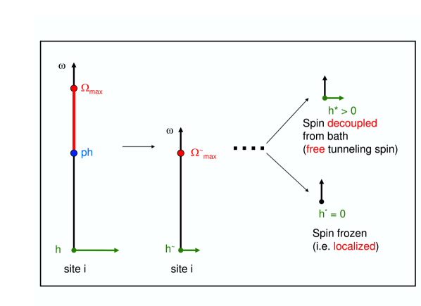
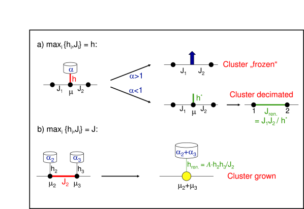
Figure 1: Left: Sketch of the adiabatic renormalization of the bosonic bath for a single spin-boson system in the Ohmic case: The fast oscillators with frequencies $\omega>ph$, where $h$ is the transverse field acting on the spin and $p$ an arbitrary large parameter, are treated in the adiabatic approximation resulting in a renormalized transverse field $\tilde{h}$ for the spin and a decreased upper cut-off frequency $\tilde{\Omega}_{\rm max}$ for the bosonic bath. This procedure is continued until it runs into a fixed point, where either the renormalized field $h^{*}$ vanishes (for $\alpha>1$) and the spin is frozen, or the renormalized field $h^{*}$ has a positive value, in which case it is a nonfrozen spin in a transverse field $h^{*}$, decoupled from the bath. Right: Sketch of the SDRG in the presence of a dissipative bath for the Ohmic case. When a field $h$ is the largest coupling (top), first the oscillator bath is renormalized along the lines sketch on the left site. Once this is done and the field is still the largest coupling the spin gets decimated as described in the text. When a bond $J$ between two spins at site 2 and 3 is the largest coupling the two spins get decimated to form a cluster with moment $\mu_{2}+\mu_{3}$, coupled to a combination of bath 2 and 3, i.e. a new dissipative bath with coupling strength $\alpha_{2}+\alpha_{3}$.

2.2 Numerical implementation.

In the following we analyze this RG procedure defined by the decimation rules (23-25, 27-30) numerically. This is done by considering a finite system of linear size $L$ with pbc and iterating the decimation rules until only one site is left. This numerical implementation has been widely used in previous works [3, 29], and it has been shown to reproduce with good accuracy the exact results of Ref. [4] for the RTFIC [29]. In particular, the transverse field $h$ acting on the last remaining spin is, at low ferromagnetic coupling $J_{0}$, an estimate for the smallest excitation energy. Its distribution, $P_{L}(h/\Gamma_{0})$, where $\Gamma_{0}$ is the largest coupling in the initial system of linear size $L$, reflects the characteristics of the gap distribution [8]. This quantity, and specifically its dependence on the system size $L$ can be efficiently used to characterize Griffith-Mc Coy singularities and critical behavior characterized by an infinite randomness fixed point.

3 Ohmic dissipation.

Ohmic dissipation means $s=1$ in (2), i.e. a spectral function for the oscillators that is linear in the frequency (up to the upper cut-off $\Omega$). For a single spin in a transverse field $h$ and coupled to such an Ohmic bath, a lot of results are available [21]. Here we mention only that this system has a phase transition at zero temperature driven by the coupling strength $\alpha$. For small $\alpha$ the spin can still tunnel quantum mechanically, whereas for large $\alpha$ the spin is frozen and behaves classically, the critical coupling strength $\alpha_{c}(h)$ is equal to $1$ in the limit where $h/\Omega\ll 1$ where $\Omega$ is the cut-off frequency of the bath, an exact result predicted correctly by the adiabatic approximation mentioned above. Such a transition is also present in an infinite ferromagnetic spin chain coupled to a dissipative bath, as it was shown recently numerically [30]. Here we want to focus on the interplay of disorder, quantum fluctuations and dissipation and study random transverse field Ising systems coupled to a dissipative environment by implementing the decimation rules (23-25, 27-30) for ohmic dissipation. For $s=1$, the amplitudes ${\cal A}$ in Eq. (18) and ${\cal A}^{\prime}$ in Eq. (28) which enter these decimation rules are given by

$${\cal A}=\left(\frac{pJ_{2}}{{\Omega}_{2}}\right)^{\alpha_{2}}\left(\frac{pJ_{2}}{{\Omega}_{3}}\right)^{\alpha_{3}}\;,\;{\cal A}^{\prime}=\left(\frac{ph_{2}}{\Omega_{2}}\right)^{\alpha_{2}}\;.$$ (31)

3.1 One dimensional system : Random transverse field Ising chain.

3.1.1 Gap distribution : finite size analysis.

The RTFIC coupled to a ohmic bath was treated in detail in Ref. [25]. We just recall here the main results. Since the last spin can either be frozen (i.e the last field $h$ is zero) or non-frozen we split $P_{L}(h/\Gamma_{0})$ into two parts:

$$P_{L}(h/\Gamma_{0})=A_{L}\tilde{P}_{L}(h/\Gamma_{0})+(1-A_{L})\delta(h/\Gamma_{0})\;,$$ (32)

where $\tilde{P}_{L}(h/\Gamma_{0})$ is the restricted distribution of the last fields in the samples that are non-frozen and $A_{L}$ is the fraction of these samples. It, or equivalently $\tilde{P}_{L}(\log(\Gamma_{0}/h))$, represents the distribution of the smallest excitation energy in the ensemble of non-localized spins. At low coupling (small $J_{0}$ or small $\alpha$), $\tilde{P}_{L}(\log(\Gamma_{0}/h))$ shows indications of Griffiths-McCoy singularities characterized by the following scaling behavior for $\tilde{P}_{L}$

$$\tilde{P}_{L}(\log(\Gamma_{0}/h))={\cal P}(\log(\Gamma_{0}/hL^{z}))\;,$$ (33)

where $z$ is a dynamical exponent continuously varying with ($J_{0}$, $\alpha$, etc.). As the coupling is increased, $z$ is also increasing and eventually, at some pseudo-critical point, $\tilde{P}_{L}(\log(\Gamma_{0}/h))$ exhibits a scaling which is characteristic for an IRFP:

$$\tilde{P}_{L}(\log(\Gamma_{0}/h))=L^{-\psi}{\cal P}_{\rm{IRFP}}(L^{-\psi}\log(\Gamma_{0}/h))$$ (34)

whith $\psi\simeq 0.32$ [25] is a critical exponent characterizing the IRFP. Notice that this value of $\psi$ is different from $\psi_{\rm RTFIC}=1/2$ computed exactly for the RTFIC [4]. The main striking point in the case of ohmic dissipation is that although the restricted distribution $\tilde{P}_{L}(\log(\Gamma_{0}/h))$ displays Griffith’s like behavior like in Eq. (33) the magnetization becomes finite above a certain length scale $L^{*}$. This finite magnetization is a manifestation of the “frozen” clusters which lead to the concept of rounded quantum phase transitions in the presence of dissipation [23]. Due to these “frozen” clusters, the amplitude $A_{L}$ decays exponentially above $L^{*}$, with $A_{L}\propto e^{-L/L^{*}}$. However, as we pointed out in Ref. [25], the interpretation of the finite size analysis (32,33,34) in presence of dissipation has to be done carefully. Indeed in Ref. [25] we suggested that despite the presence of these frozen clusters, Griffith’s singularities should be observable in the susceptibility $\chi(T)$, above a certain temperature $T^{*}\propto L^{*-z}$ as well as in the specific heat $C_{v}(T)$. This property can actually be shown (see A) on a toy model where one considers a RTFIC without dissipation but with a finite fraction $\rho$ of zero transverse fields.

Here we will use this strong disorder approach to extract thermodynamical properties of the full problem described by the Hamiltonian (3).

3.1.2 Susceptibility at finite temperatures.

The SDRG successively eliminates degrees of freedom with a large excitation energy from the starting Hamiltonian, thereby reducing continuously the maximum energy scale of the effective Hamiltonian. If continued down to the smallest energy scale the final effective Hamiltonian (consisting only of a single but large cluster in an effective transverse field) provides information about the ground state of the starting spin chain, the gap, the size, the geometry, etc… of the smallest excitation energy. To extract information on thermodynamic properties, at low but non-vanishing temperatures, one has to stop the RG procedure at an energy scale of the same order of magnitude as the temperature $T$: clusters (or degrees of freedom) that are already frozen at this energy scale will not be active at this temperature and behave like classical spins (at this temperature). The thermodynamical properties, observables like susceptibility or specific heat, will be determined by the active, i.e. not yet frozen clusters.

It is instructive to have a look at the number and size of frozen clusters as a function of the upper cut-off energy, which we identify now with the temperature $T$. As one can see from the left panel of Fig. 2 the number of frozen clusters is zero at high temperatures (simply because $\alpha<1$) and increases rapidly with decreasing temperature before it reaches a maximum and then decreases. The initial increase is due to the formation of many small clusters that behave like classical spins at the corresponding temperature with moments of the order of $10$. The subsequent decrease of the number of clusters correlates with an increase in the size of the clusters as can be seen in th right panel of Fig. 2 and which is due to the coalescence of small clusters into larger ones at the corresponding temperatures.

Figure 2: Number (left) and size (right) of frozen clusters in the disordered chain coupled to an ohmic bath as a function of temperature $T$ for different values of $\alpha$. Shown are data for a single large disorder realization, the size is $L=40000$, the disorder strength is $h_{0}=1$, $J_{0}=0.025$. For this value of $J_{0}$ the pseudo critical point is located at $\alpha=0.2$ [25].

With this picture in mind we estimate the zero frequency susceptibility $\chi(T)$, as the sum of two contributions $\chi(T)=\chi_{\rm active}(T)+\chi_{\rm frozen}(T)$, one arising from the active, i.e. non “frozen” spins, $\chi_{\rm active}(T)$ and one from the “frozen” ones, $\chi_{\rm frozen}(T)$. In doing this, we assume that the interaction between the frozen and the non frozen clusters is negligible. $\chi_{\rm active}(T)$ is given by (see also Eq. (53)):

$$\chi_{\rm active}(T)=\int_{0}^{\infty}\frac{d\epsilon}{\epsilon}\rho(\epsilon)(1-\exp{(-\beta\epsilon}))$$ (35)

with $\beta=1/T$. To estimate the density of states $\rho(\epsilon)$ using our RG scheme we compute the distribution of the amplitudes of fields and bonds which are decimated during the renormalization procedure [1]. Having computed $\rho(\epsilon)$, we then perform numerically the integration in Eq. (35) to compute $\chi_{\rm active}(T)$. In the Griffith’s region where the restricted distribution scales with $L$ as in Eq. (33), one has $\rho(\epsilon)\propto\epsilon^{-1+1/z}$ and thus $\chi_{\rm active}(T)\propto T^{-1+1/z}$. On the other hand, each (quantum mechanically) frozen spin contributes the susceptibility by an amount of $1/T$ and thus

$$\chi_{\rm frozen}(T)=\frac{{\cal N}_{\rm frozen}(T)}{T}$$ (36)

where ${\cal N}_{\rm frozen}(T)$ denotes the number of frozen spins at temperature $T$ and its finite $T$ dependence is computed as explained above. We have computed $\chi(T)$ using our RG scheme for a system of size $L=4096$ for different values of $\alpha=0.15,0.17,0.19,0.20$ and $0.22$ for $J_{0}=0.025$. In each case, $\chi(T)$ is averaged over $10^{4}$ different realizations of the random couplings and the plots are shown on the left panel of Fig. 3.

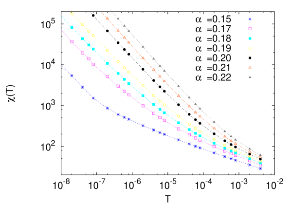
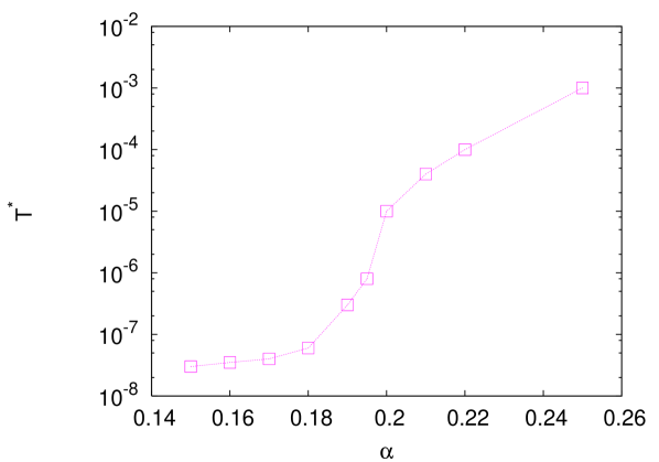
Figure 3: Left: Magnetic susceptibility $\chi(T)$ for a disordered chain coupled to an ohmic bath as a function of temperature for different coupling strength $\alpha$. The susceptibility is calculated as $\chi(T)=\chi_{\rm active}(T)+\chi_{\rm frozen}(T)$ using Eq. (35) and Eq. (36). The size is $L=4096$, the disorder strength is $h_{0}=1$, $J_{0}=0.025$. For this value of $J_{0}$ the pseudo-critical point is located at $\alpha=0.2$ [25] Right: Crossover temperature $T^{*}$ as a function of $\alpha$ extracted from the data on the left panel by the condition $\chi_{\rm active}(T^{*})=\chi_{\rm frozen}(T^{*})$ (see text).

Let us first consider the curves for $\alpha<0.2$, where the restricted distribution $\tilde{P}_{L}(\log(\Gamma_{0}/h))$ shows a scaling with $L$ as in Eq. (33) [25]. For low temperatures still above some temperature $T^{*}$, $T>T^{*}$, one sees in the left panel of Fig. 3 that $\chi(T)$ is dominated by $\chi_{\rm active}(T)\propto T^{-1+1/z}$, for $\alpha<0.2$. In this regime of dissipation, one observes that the slope of $\chi(T)$ in a log-log plot depends on $\alpha$: this is the characteristics of Griffith’s behavior. At lower temperature $T<T^{*}$, $\chi(T)$ is dominated by the $1/T$ behavior of $\chi_{\rm frozen}(T)$ coming from the frozen clusters. Thus Fig. 3 shows that Griffith’s behavior can indeed be observed above $T^{*}$. For $\alpha>0.2$, the susceptibility behaves like $\chi(T)\sim 1/T$ in the whole range of temperature.

In addition, given that we compute separately $\chi_{\rm active}(T)$ in Eq. (35) and $\chi_{\rm frozen}(T)$ in Eq. (36) our numerical RG procedure allows to estimate $T^{*}$ for which these two contributions are equal, $\chi_{\rm active}(T^{*})=\chi_{\rm frozen}(T^{*})$. In the right panel of Fig. 3, we show a plot of $T^{*}$ as a function of $\alpha$. One observes in particular that $T^{*}$ shows an inflexion point as the pseudo-critical point is crossed such that $T^{*}$ is actually quite small in the Griffith’s region.

We now turn to the specific heat $C_{v}(T)$ of the spin degrees of freedom. Assuming that one can also neglect the interaction between frozen and non frozen clusters one immediately obtains that $C_{v}(T)=C_{v,{\rm active}}(T)$ given that $C_{v,{\rm frozen}}(T)=0$. $C_{v}(T)$ is thus

$$C_{v}=\frac{\partial{\cal E}(T)}{\partial T}$$ (37)

$${\cal E}(T)-{\cal E}(T=0)=\frac{1}{L}\int_{0}^{\infty}\;d\epsilon\;\rho(\epsilon)\,\epsilon\frac{\exp{(-\beta\epsilon)}}{1+\exp{(-\beta\epsilon)}}$$ (38)

where ${\cal E}(T)$ is the internal energy at temperature $T$. In the Griffith’s region where the restricted gap distribution has a finite $L$ scaling as in Eq. (33), one expects ${\cal E}(T)-{\cal E}(T=0)\propto T^{1+1/z}$, thus $C_{v}(T)\propto T^{1/z}$ without any cut-off at some temperature $T^{*}$. In analogy to $\chi(T)$ we have computed numerically ${\cal E}(T)-{\cal E}(T=0)$ (also averaged over $10^{4}$ disordered samples) for different values of $\alpha$. On Fig. 4 we show a plot of $T^{-1}({\cal E}(T)-{\cal E}(T=0))\propto C_{v}(T)$ as a function of $T$ for different values of $\alpha$. One observes clearly that the slope decreases as $\alpha$ is increased, i.e. as the critical point is reached. We tried to extract an estimate of the dynamical exponent $z$ by fitting the curves in Fig. 4 by $T^{-1}({\cal E}(T)-{\cal E}(T=0))\propto T^{1/z}$ at low $T$ as well as by fitting the curves in the left panel of Fig. 3 by $\chi(T)\propto T^{-1+1/z}$ for $T>T^{*}$. Both estimates for $z$ coincide approximately but since the data shown are close to the pseudo-critical point (which corresponds here to $\alpha=0.2$), it is rather hard to extract properly the dynamical exponent given that $1/z$ becomes quite small, thus one would certainly need smaller temperatures to obtain a reliable estimate of $z$.

We conclude this paragraph by noting that the data in Fig. 3 and 4 indicate that Griffith’s behavior of thermodynamical quantities is observable also in the presence of dissipation.

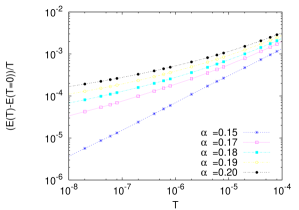
Figure 4: The scaled energy $T^{-1}({\cal E}(T)-{\cal E}(T=0))$, which is proportional to the specific heat $C_{v}(T)$, for the disordered chain coupled to an ohmic bath as a function of temperatur $T$ in a log-log plot. Copmputations are done using Eq. (38). The different curves correspond to different values of $\alpha$. Note that the low temperature behavior is characterized by different slopes for different $\alpha$, corresponding to a varying exponent $1/z$. The system size is $L=4096$, the disorder strength $h_{0}=1$, $J_{0}=0.025$. For this value of $J_{0}$ the pseudo critical point is located at $\alpha=0.2$ [25].

3.2 Disordered ladder.

Our previous study on Ref. [25] was restricted to the one dimensional case. Here, we implement numerically the real space renormalization defined by Eq. (23-25) and Eq. (27-30) for a disordered ladder coupled to a dissipative bath. When considering a ladder (as well as a two-dimensional square lattice) these decimation rules have to be slightly modifed to take into account the topology of the system [29]. First, Eq. (25) has to be modified. In this case, the two spins $2$ and $3$ are combined to a cluster but when we compute the interactions between this cluster and the rest of the chain, one has to consider the case in which the two original spins $2$ and $3$ were actually coupled to the same spin $i$. Although this does not happen in the initial ladder, such a situation may occur during later stages of the renormalization. In this case we set the ferromagnetic coupling of this spin $i$ with the newly formed cluster to

$$\tilde{J}_{i,{\rm cluster}}={\rm max}(J_{i2},J_{i3})\;.$$ (39)

The sum of the two bond strengths could also be taken, but does not make a significant difference when the probability distribution of the bond strengths is broad.

The decimation rule on Eq. (30) has also to be modified. This rule says that when the spin on site $2$ is decimated, effective interactions are generated between the neighboring sites of $2$. But during renormalization of the ladder there might already be bonds $J_{ij}$ present between neighboring sites $i$ and $j$ of site $2$. In this case we replace Eq. (30) by

$$\tilde{J}_{ij}\simeq{\rm max}(J_{ij},\frac{J_{i2}J_{2j}}{h_{2}})\;.$$ (40)

The topology of the system changes drastically under renormalization. One starts with a ladder and the decimations change its structure into a random graph, but this change is straightforward to implement numerically.

In the absence of dissipation a critical point was found for $h_{0}=1.9,J_{0}=1$ [29]. In the following we fix $h_{0}=1.9$ and $J_{0}=0.001$ and we vary $\alpha$. As it was done previously for the disordered chain in Ref. [25] we first focus on the restricted distribution of the last fields in the samples that are non frozen (32). For small $\alpha$, $\tilde{P}_{L}(h/\Gamma_{0})$ displays Griffith’s like behavior as in Eq. (33). In the left panel of Fig. 5, one plots $\tilde{P}_{L}(h/\Gamma_{0})$ as a function of $\log(\Gamma_{0}/hL^{z})$ with $z=1.7$ for different system sizes $L=64,128,256,512$ for $\alpha=0.2$. The good data collapse of the curves for different $L$ is in a good agreement with Griffith’s scaling (33).

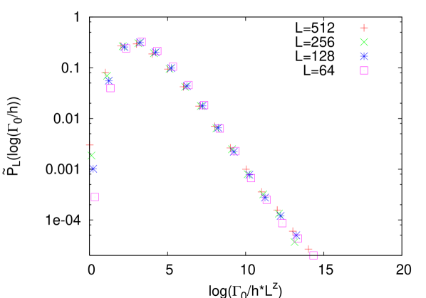
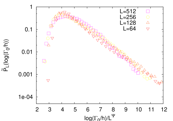
Figure 5: Scaling plot of the restricted distribution $\tilde{P}_{L}(h/\Gamma_{0})$ of the last field to be decimated in the non-frozen samples for the disordered ladder coupled to an ohmic bath. Here $h_{0}=1.9$, $J_{0}=0.001$. Left: In the Griffiths-region ($\alpha=0.27$): $\tilde{P}_{L}(h/\Gamma_{0})$ as a function of $\log(\Gamma_{0}/hL^{z})$ for different system sizes $L$. The best data collapse is obtained with the dynamical exponent $z=1.7$. Right: At the pseudo-critical point ($\alpha=0.27$): $L^{\psi}\tilde{P}_{L}(\Gamma_{0}/h)$ as a function of $\log{(\Gamma_{0}/h)}/L^{\psi}$ for different system sizes $L$. The best data collapse is obtained with the exponent $\psi=0.27(3)$.

We observe that the dynamical exponent $z$ increases with increasing $\alpha$. This is depicted in the left panel of Fig. 6 where one plots again $\tilde{P}_{L}(h/\Gamma_{0})$ as a function of $\log(\Gamma_{0}/hL^{z})$ for different system sizes $L$ but with $z=7.5$ for $\alpha=0.262$.

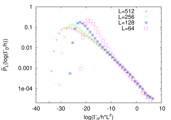
Figure 6: Left: Scaling plot of the restricted distribution $\tilde{P}_{L}(h/\Gamma_{0})$ of the last field to be decimated in the non-frozen samples for the disordered ladder coupled to an ohmic bath. Here $h_{0}=1.9$, $J_{0}=0.001$ and $\alpha=0.262$, i.e. close to the pseudo-critical point at $\alpha=0.27$. The best data collapse is obtained by the dynamical exponent $z=7.5$. Right: Magnetic moment $\mu(L)$ as a function of $L$ in the Griffith’s region (parameters as in the left panel). The linear behavior implies a non-vanishing magnetization $m_{\rm eq}$ per spin.

However, despite the fact that the gap distribution displays Griffith’s behavior, the magnetization is already finite. This can be seen by computing the magnetic moment of the last remaining cluster as a function of the system size $L$, see the right panel of Fig. 6. This behavior, which is due to frozen clusters is very similar to the one observed for the disordered chain [25].

Finally, one reaches a value of $\alpha$ where $z$ is diverging and one observes a scaling characteristic for an infinite randomness fixed point as in Eq. (34). This is shown on the right panel of Fig. 5 where we plot $L^{\psi}\tilde{P}_{L}(\Gamma_{0}/h)$ as a function of $\log{(\Gamma_{0}/h)}/L^{\psi}$ with $\psi=0.27(3)$.

3.3 Two-dimensional square lattice.

We have also implemented the decimation rules in two dimensions for a square lattice. Here also the topology of the system changes drastically during renormalization. In the absence of dissipation a critical point was found for $h_{0}=5.35,J_{0}=1$. Here we include dissipation, fix $J_{0}=0.0001$ and vary $\alpha$. At small $\alpha$ one observes Griffith’s like behavior of the restricted distribution as in Eq. (33). In the left panel of Fig. 7, we plot $\tilde{P}_{L}(\log(\Gamma_{0}/h))$ as a function of $\log{(\Gamma_{0}/h)}$ for different system sizes $L=8,16,32,64$ and $\alpha=0.3$. On the right panel, we show that these curves for different fall $L$ on a master curve if one plots them as a function of $\log(\Gamma_{0}/hL^{z})$ with $z=3.1$.

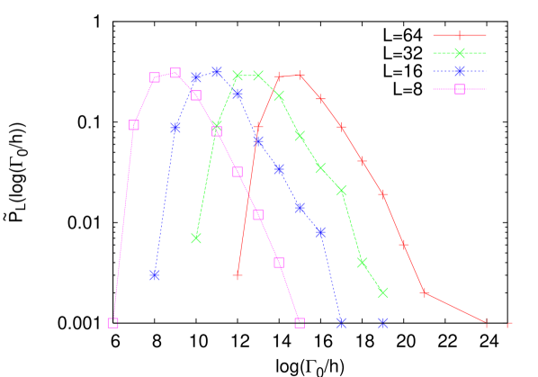
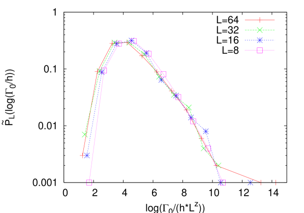
Figure 7: The restricted distribution $\tilde{P}_{L}(h/\Gamma_{0})$ of the last field to be decimated in the non-frozen samples for the disordered square lattice coupled to an ohmic bath. Parameter values fall into the Griffiths-region: the disorder strength is $h_{0}=5.35$, $J_{0}=0.0001$ and the coupling to the bath is $\alpha=0.3$. Left: $\tilde{P}_{L}(\log(\Gamma_{0}/h))$ as a function of $\log{(\Gamma_{0}/h)}$ for different system sizes $L$. Right: Scaling plot of the data in the left panel: $\tilde{P}_{L}(\log(\Gamma_{0}/h))$ as a function of $\log(\Gamma_{0}/hL^{z})$ for different system size $L$. The best data collapse is obtained with $z=3.1$.

As we increase the value of $\alpha$, one observes that $z$ is also increasing and eventually we identify a pseudo critical point, here for $\alpha=0.37$, where the restricted distribution has a scaling form characteristic for an IRFP as in Eq. (34) with $\psi=0.32$. This is shown in Fig. 8.

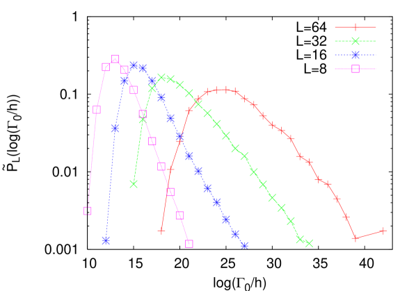
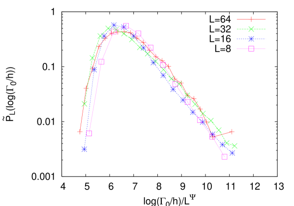
Figure 8: The restricted distribution $\tilde{P}_{L}(h/\Gamma_{0})$ of the last field to be decimated in the non-frozen samples for the disordered square lattice coupled to an ohmic bath. Parameter values correspond to the pseudo-critical point: the disorder strength is $h_{0}=5.35$, $J_{0}=0.0001$ and the coupling to the bath is $\alpha=0.37$. Left: $\tilde{P}_{L}(\log(\Gamma_{0}/h))$ as a function of $\log{(\Gamma_{0}/h)}$ for different system size $L$. Right: Scaling plot of the data in the left panel: $\tilde{L}^{\psi}P_{L}(\log(\Gamma_{0}/h))$ as a function of $\log(\Gamma_{0}/h)/L^{\psi}$. The best data collapse is obtained with the exponent $\psi=0.32$.

4 Super-ohmic dissipation.

We have implemented numerically the decimation rules for the super-ohmic bath, which corresponds to $s>1$. In this case the amplitude ${\cal A}$ in Eq. (18) and ${\cal A}^{\prime}$ in Eq. (28) which enter the decimation rules are given by

$${\cal A}=\exp{\left(-\frac{\alpha_{2}}{s-1}\left(1-\left(\frac{pJ_{2}}{\Omega_{2}}\right)^{s-1}\right)-\frac{\alpha_{3}}{s-1}\left(1-\left(\frac{pJ_{2}}{\Omega_{3}}\right)^{s-1}\right)\right)}\;,$$

$${\cal A}^{\prime}=\exp{\left(-\frac{\alpha_{2}}{s-1}\left(1-\left(\frac{ph_{2}}{\Omega_{2}}\right)^{s-1}\right)\right)}\;.$$ (41)

For $s>1$ iterations of the decimation rules (27) always converge to a fixed point value $h_{2}^{*}>0$ given in Eq. (29). Consequently, the spins can not be frozen by the dissipative bath.

We first present results for $s=3$, which corresponds to a phonon bath, and one fixes the coupling to te bath to $\alpha=0.5$ and the strength of the random transverse field to $h_{0}=1.0$. All data presented here were obtained by averaging over $10^{4}$ different realizations of the disordered couplings.

We first focus on low value of $J_{0}$. In Fig. 9, one shows a plot of $P_{L}(\Gamma_{0}/h)$, the distribution of the transverse field acting on the last remaining cluster as a function of $\log(\Gamma_{0}/hL^{z})$ for different system sizes with $z=2.87$. The good data collapse of these different curves suggests that $P_{L}(h/\Gamma_{0})$ exhibits Griffith’s behavior:

$$P_{L}(\log(\Gamma_{0}/h))={\cal P}(\log(\Gamma_{0}/hL^{z}))\;.$$ (42)

Notice that, at variance with the case of ohmic dissipation (32) one has here $A_{L}=1$.

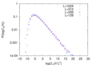
Figure 9: Scaling plot of the probability distribution of the last decimated field for the disordered chain with super-ohmic dissipation, here $s=3$: $P_{L}(\Gamma_{0}/h)$ vs. $\log{(\Gamma_{0}/hL^{z})}$ (scaling in the Griffiths region) for different system size $L$. The best data collapse is obtained with $z=2.87$. The disorder strength is $h_{0}=1.0$ and $J_{0}=0.55$ and the coupling to the bath is $\alpha=0.5$.

If one increases $J_{0}$, $z$ is also increasing and for some critical value of $J_{0}=J_{0c}$, here $J_{0c}=0.78$ one observes a scaling characteristic for an IRFP

$$P_{L}(\log(\Gamma_{0}/h))=L^{-\psi}{\cal P}_{\rm{IRFP}}(L^{-\psi}\log(\Gamma_{0}/h))\;,$$ (43)

with $\psi=1/2$ as in the case without dissipation [4]. This is shown in the left panel of Fig. 10.

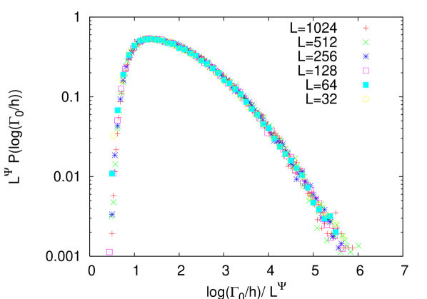
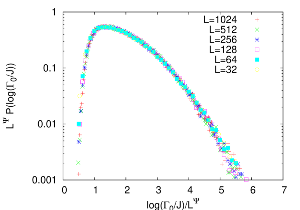
Figure 10: Left: Scaling plot of the probability distribution of the last decimated field for the disordered chain with super-ohmic dissipation, here $s=3$: $L^{\psi}P_{L}(\log(\Gamma_{0}/h))$ vs. $(\log(\Gamma_{0}/h))/L^{\psi}$ (IFRP scaling) for different system size $L$ with $\psi=1/2$. The disorder strength is $h_{0}=1.0$ and $J_{0}=0.55$ and the coupling to the bath is $\alpha=0.78$. Right: The same as in the left panel but for the bond distribution instead of the field distribution. Note the similarity of the two distributions.

In the absence of dissipation random fields and random bonds play a symmetric role in the RTFIC. This is in principle not the case when one includes dissipation in the Hamiltonian (1). However, this symmetry is restored asymptotically, close to the critical point. To show this, we have computed $P_{L}(J/\Gamma_{0})$ where $J$ is the last decimated bond. In Fig. 10 we show a plot of $L^{\psi}P_{L}(\log(\Gamma_{0}/J))$ as a function of $(L^{-\psi}\log(\Gamma_{0}/h))$ with $\psi=1/2$ for $J_{0}=J_{0c}$. The good data collapse, together with the similarities between the plots shown on both panels of Fig. 10 suggest indeed that this symmetry between bonds and fields is restored at the critical point.

To characterize this IRFP, we have also computed the combinations of the products of the exponents $\varphi\psi$ where $\varphi$ is another independent exponent associated to this IRFP. This can be measured by computing the disorder averaged correlation function $C(r)$ at the transition. We compute it by keeping track of the clusters during the decimation procedure and compute $C(r)=L^{-1}\sum_{i}w_{i,i+r}$ where $w_{i,j}=1$ if the sites $i$ and $j$ belong to the same cluster, and $w_{i,j}=0$ otherwise. We have checked that for RTFIC without dissipation at the critical point this gives the correct exponent [4] within $5\%$ accuracy. A plot of $C(r)$ is shown on Fig. 11 for different system sizes $L=64,128,256,512$ and $1024$. This plot shows that $C(r)\propto r^{-\eta}$ with $\eta=0.38(1)$, as in the case without dissipation [4].

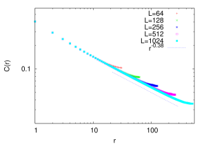
Figure 11: The disorder averaged correlation function $C(r)$ at the critical point for the chain coupled to a super-ohmic bath (here $s=3$) for different system size $L$. The disorder strength is $h_{0}=1$ and $J_{0}=0.78$ and the coupling to the bath is $\alpha=0.5$. The error bars are smaller than the size of the symbols. The decay exponent $\simeq 0.38$ gives $\phi\psi\simeq 0.81$ as in the case without dissipation [4].

We have repeated the same procedure for different values of $s$ and found the critical value $J_{0c}(s)$. We thus obtain the phase diagram in the plane $(J_{0},1/s)$ shown in Fig. 12 where a critical line separates a paramagnetic phase from a ferromagnetic one.

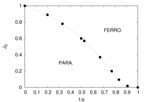
Figure 12: Phase diagram for a disordered chain coupled to a super-ohmic bath (except for $s=1$) and $h_{0}=1,\alpha=0.5$. The error bars are smaller than the size of the symbols. Along the line the critical behavior is governed by an IRFP with $\psi=1/2$ (see Fig. 10 above). The dashed line is the exact expression of the critical coupling given in the text (44).

Along this line, we have found a scaling like in Eq. (43) with an exponent $\psi=1/2$, independently of $s$. One can actually estimate the shape of the critical line in Fig. 12 by assuming that the main effect of dissipation is to reduce the amplitude of the random transverse field $h_{0}$ to $h_{0}^{*}$ given by Eq. (29). If one further assumes that bonds and fields play a symmetric role at the critical point (which is fully compatible with our numerical results in Fig. 10), the critical point is then given by the relation $J_{0}=h_{0}^{*}$, as in the RTFIC [4]. This leads to

$$J_{0c}=h_{0}\exp{\left(\frac{-\alpha}{s-1}\right)}\;,$$ (44)

which is actually in very good agreement with our numerical estimates for the critical line in Fig. 12. Using the same arguments, one can also derive analytically the behavior of the dynamical exponent when approaching the critical point, this yields

$$z\propto\frac{1}{2\delta}\quad,\quad\delta=\frac{1}{2}\log{\left(\frac{h_{0}e^{-\alpha/(s-1)}}{J_{0}}\right)}\;,$$ (45)

which we have checked to be in good agreement with numerical results.

Our results thus suggest that for $s>1$, the large scale $L>L_{s}$ properties of the system with super ohmic dissipation behaves at criticality as the dissipationless system. On the other hand, one expects that $L_{s}$ is diverging when $s\to 1$. To estimate its behavior close to $s=1$ one observes that the typical energy scale at criticality is given by $E_{s}\propto h_{0}\exp(-\alpha/(s-1))$ (44). But given that the critical behavior is governed by an IRFP, one expects that $L_{s}\propto(\log E_{s})^{1/\psi}$, with $\psi=1/2$, see Fig. 10. Therefore we estimate

$$L_{s}\propto\frac{\alpha^{2}}{(s-1)^{2}}\;,$$ (46)

the length above which the system with super ohmic dissipation behaves like the one without dissipation.

5 Conclusion

In this paper we have developed a real space renormalization, which combines the SDRG for strongly disordered quantum magnets with the adiabatic renormalization for spin-boson systems, to study disordered, ferromagnetically interacting transverse Ising systems coupled to a dissipative bath. In the important case of ohmic dissipation, we have first extended our previous study in Ref. [25] to describe thermodynamical properties. In particular we have shown that Griffith’s Mc-Coy singularities are visible in the spin specific heat at all temperatures and in the magnetic susceptibility above a (small) temperature $T^{*}$. For weak dissipation this temperature is extremely small and system sizes above which classical behavior in the susceptibility becomes visible are extremely large, which represents a major obstacle for numerical studies [31].

We have also shown that the disordered ladder as well as the $2d$ disordered square lattice coupled to a ohmic bath displays the same behavior. Using this real space renormalization, we also studied the case of super-ohmic dissipation ($s>1$). There we have found a quantum phase transition described by an IRFP, which is the same as the one found without dissipation. Such a scenario is expected to hold also in higher dimensions.

It would be natural to extend this approach to sub-ohmic dissipation ($s<1$). Unfortunately, it is well known that in that case the adiabatic renormalization fails to describe correctly the single spin-boson, which in itself has been the subject of recent works [32]. Therefore the problem of an infinite chain (possibly disordered) coupled to a sub-ohmic bath remains a challenging problem which surely deserves further investigations.

A final remark concerns the effect of dissipation upon magnetic systems with a continuous symmetry instead of the discrete (Ising) case we studied in this work. Griffiths-McCoy singularities are much weaker in systems with a continuous symmetry [33], and one would therefore expect that coupling to a dissipative bath would not freeze the strongly coupled regions, but enhance their singular behavior. What actually happens can elegantly be classified according to whether rare regions including their long range interactions in imaginary time due to dissipation are below, at or above their upper critical dimension [24]. A disordered itinerant antiferromagnet, for instance, was recently studied with the strong disorder renormalization group and an infinite randomness fixed point was found [34], including the accompanying algebraic Griffiths-McCoy singularities. On the other hand non-intinerant antiferromagnets, involving localized magnetic moments, in spatial dimensions larger than 2 like the Heisenberg antiferromagnet on the square lattice, will not show pronounced Griffiths-McCoy behavior since here the Neél ordered ground state is very robust against disorder [35] and no quantum critical point occurs. The effect of dissipation upon strongly disordered magnets thus depends crucially on the effect of disorder itself on the system’s ground state.

Appendix A A toy model for an Ising chain with ohmic dissipation

To understand qualitatively the full problem described by the Hamiltonian (3) with ohmic dissipation, it is instructive to consider a simpler model where one considers a RTFIC without dissipation but with a finite fraction $\rho$ of zero transverse fields. We thus study in detail in this appendix the RTFIC Hamiltonian with $k$ sites having zero transverse fields ($\rho=k/L$)

$${\cal H}=-\sum_{i=1}^{L}J_{i}\sigma_{i}^{z}\sigma_{j}^{z}+\sum_{i=1}^{L}h_{i}\sigma_{i}^{x}\qquad{\rm and}\quad h_{i_{1}}=\ldots=h_{i_{k}}=0\;.$$ (47)

First, one immediately sees that the distribution $P_{L}(h/\Gamma_{0})$ shows the same behavior as in Eq. (32) with $A_{L}\sim e^{-L/L^{*}}$ and in the small $\rho$ limit, $L^{*}\propto\rho^{-1}$. Besides, the local zero frequency susceptibility is

$$\chi_{i}(\omega=0) = \int_{0}^{\beta}d\tau\langle\sigma_{i}^{z}(\tau)\sigma_{i}^{z}(0)\rangle$$

$$= \int_{0}^{\beta}d\tau\frac{1}{\cal Z}{\rm Sp}\{\rho e^{{\cal H}\tau}\sigma_{i}^{z}e^{-{\cal H}\tau}\sigma_{i}^{z}\}$$

$$= \frac{1}{\cal Z}\sum_{\{n,m\;(E_{n}\neq E_{m})\}}\frac{e^{-\beta E_{m}}-e^{-\beta E_{n}}}{E_{n}-E_{m}}|\langle n|\sigma_{i}^{z}|m\rangle|^{2}$$

$$+ \frac{1}{\cal Z}\sum_{\{n,m\;(E_{n}=E_{m})\}}\beta e^{-\beta E_{n}}|\langle n|\sigma_{i}^{z}|m\rangle|^{2}\;,$$ (49)

where $\{|n\rangle\}$ is a complete basis of eigenvectors of ${\cal H}$ (47). Their corresponding eigenvalues $E_{n}$ are such that $E_{0}<E_{1}<E_{2}<...$. The first term in Eq. (49) yields at zero temperature in the non-degenerate case (all transverse fields positive, finite system size $L$) the known formula

$$\chi_{i}^{T=0}(\omega=0)=2\sum_{n\neq 0}\frac{|\langle n|\sigma_{i}^{z}|0\rangle|^{2}}{E_{n}-E_{0}}\;,$$ (50)

since then $\langle 0|\sigma_{i}^{z}|0\rangle=0$ and the last term in Eq. (49) vanishes.

If one or more transverse fields vanish the Hamiltonian becomes block-diagonal. We choose $z$-representation, such that states can be denoted $\psi=|S_{1},\ldots,S_{L}\rangle$, with $S_{i}=\pm 1$. For convenience we permute the components such that the site $i_{1},\ldots,i_{k}$ with the $k$ vanishing transverse fields $h_{i_{1}},\ldots,h_{i_{k}}$ stand to the left: $\psi=|S_{i_{1}},\ldots,S_{i_{k}},S_{j_{1}},\ldots,S_{j_{L-k}}\rangle$. All $2^{k}$ blocks are identical up to the diagonal part $-\sum_{i}J_{i}S_{i}S_{i+1}$. As a result the two blocks belonging to the states with $S_{i_{1}}=\ldots=S_{i_{k}}$ (ferromagnetically aligned “frozen” spins), have the lowest ground state energy. Obviously

$$\langle\psi|\sigma_{i_{p}}^{z}|\psi\rangle = S_{i_{p}}\quad{\rm for}\quad p=1,\ldots,k$$ (51)

$$\langle\psi|\sigma_{i}^{z}|\psi^{\prime}\rangle = 0\quad{\rm for}\quad i=1,\ldots,L,$$

$$\quad{\rm and}\quad(S_{i_{1}},\ldots,S_{i_{k}})\neq(S_{i_{1}}^{\prime},\ldots,S_{i_{k}}^{\prime})\;.$$

At low temperatures ($T\to 0$) the main contributions in the sums in (49) comes form the terms with $E_{n}=E_{0}$ or $E_{m}=E_{0}$, the ground state energy. When $k\neq 0$ there are two ground states $|0_{S}\rangle$, one with $S=+1$, one with $S=-1$. For $T\to 0$ ${\cal Z}$ can be replaced by $2e^{-\beta E_{0}}$, since ${\cal Z}=2e^{-\beta E_{0}}(1+\sum_{m}e^{-\beta(E_{m}-E_{0})})$. The two ground states produce also an extra factor 2 (in addition to the one for the sum over $n\neq m$, where either $|n\rangle$ or $|m\rangle$ can be the ground state):

$$\chi_{i}(\omega=0) = \frac{4}{2e^{-\beta E_{0}}}\sum_{n\neq 0}\frac{e^{-\beta E_{0}}-e^{-\beta E_{n}}}{E_{n}-E_{0}}|\langle n|\sigma_{i}^{z}|0\rangle|^{2}+\frac{2}{2e^{-\beta E_{0}}}\,\beta\,e^{-\beta E_{0}}|\langle 0|\sigma_{i}^{z}|0\rangle|^{2}$$ (53)

$$= 2\sum_{n\neq 0}\frac{1-e^{-\beta(E_{n}-E_{0})}}{E_{n}-E_{0}}|\langle n|\sigma_{i}^{z}|0\rangle|^{2}+\beta|\langle 0|\sigma_{i}^{z}|0\rangle|^{2}\;.$$

The usual argument leading to $\chi_{i}(\omega=0)\propto T^{-1+1/z}$ in the Griffiths-McCoy phase of the RTFIC with $k=0$ involves neglecting the terms $n>1$ in the first sum in (53). This leads to $\chi_{i}(\omega=0)\sim(\Delta E)^{-1}$, where $\Delta E=E_{1}-E_{0}$ is the gap, which follows the distribution $P(\Delta)\sim\Delta^{-1+1/z}$. In the present case this distribution has a cut-off at $\Delta_{\rm min}$ that is exponentially small in $L^{*}$, the average distance between sites with zero transverse fields. Thus one expects the first term of (53) to display $T^{-1+1/z}$-behavior down to a temperature $T_{\rm min}=\Delta_{\rm min}^{z/(z-1)}\sim e^{-aL^{*}}$. The second term is $\beta\cdot m_{i}^{2}$, where $m_{i}$ is the local magnetization in (one of) the ground states - and is non-zero due to (51). It decays exponentially with the distance $x$ from the nearest frozen site $i_{p}$: $m_{i}~{}e^{-x/2}$, thus the average over all sites is approximately

$$[m_{i}^{2}]_{\rm av}\sim\frac{1}{L^{*}/2}\int_{0}^{L^{*}/2}dx\,e^{-x}\sim\frac{1}{L^{*}}.$$ (54)

Thus a $T^{-1}$-behavior coming from the second term in (53) with amplitude of order $1/L^{*}$ competes with a $T^{-1+1/z}$-behavior with amplitude of order $1$ coming from the first term in (53). The latter dominates for temperatures above a cross-over temperature $T_{\rm cross}$, which is given by

$$T_{\rm cross}\sim(L^{*})^{-z}\;,$$ (55)

which is larger then $T_{\rm min}$ (caused by the finite average length $L^{*}$ of the segments) but still very small when $L^{*}\gg 1$ (for instance for $L^{*}=10^{3}$ and $z=2$ one has $T_{\rm cross}\sim 10^{-6})$.

References

- [1] Fisher D S 1999 Physica A 263 222
- [2] [] Motrunich O, Mau S-C, Huse D A and Fisher D S 2000 Phys. Rev. B 61 1160
- [3] Iglói F and Monthus C 2005 Phys. Rep. 412 277
- [4] Fisher D S 1992 Phys. Rev. Lett. 69 534
- [5] []Fisher D S 1995 Phys. Rev. B 51 6411
- [6] Rieger H and Young A P 1996 Phys. Rev. B 54 3328
- [7] []Guo M, Bhatt R N and Huse D A 1996 Phys. Rev. B 54 3336
- [8] Young A P and Rieger H 1996 Phys. Rev. B 53 8486
- [9] []Iglói F and Rieger H 1998 Phys. Rev. B 57 11404
- [10] Iglói F, Juhász R and Rieger H 1999 Phys. Rev. B 59 11308
- [11] []Iglói F, Juhász R and Rieger H 2000 Phys. Rev. B 61 11552
- [12] Pich C, Young P A, Rieger H and Kawashima N 1998 Phys. Rev. Lett. 81 5916
- [13] []Rieger H and Kawashima N 1999 Europ. Phys. J. B 9 233
- [14] Andrade M C et al. 1998 Phys. Rev. Lett. 81 5620
- [15] [] Castro Neto A H, Castilla G and Jones B A 1998 Phys. Rev. Lett. 81 3531
- [16] Stewart G R 2001 Rev. Mod. Phys. 73 797
- [17] Castro Neto A H and Jones B A 2000 Phys.Rev.B 62 14975
- [18] [] Castro Neto A H and Jones B A 2005 Europhys. Lett. 71 790
- [19] Millis A J, Morr D K and Schmalian J 2001 Phys. Rev. Lett. 87 167202
- [20] []Millis A J, Morr D K and Schmalian J 2002 Phys. Rev. B 66 174433
- [21] Legget A et al. 1987 Rev. Mod. Phys. 59 1
- [22] Berche B, Berche P E, Iglói F and Palágyi G 1998 J. Phys. A 31 5193
- [23] Vojta T 2003 Phys. Rev. Lett. 90 107202
- [24] Vojta T 2006 J. Phys. A 39 R143
- [25] Schehr G and Rieger H 2006 Phys. Rev. Lett. 96 227201
- [26] Ma S K, Dasgupta C and Hu C K 1979 Phys. Rev. Lett. 43 1434
- [27] [] Dasgupta C and Ma S K 1980 Phys. Rev. B 22 1305
- [28] Bulla R, Lee H J, Tonh N H and Vojta M 2005 Phys. Rev. B 71 045122
- [29] Lin Y C, Kawashima N, Igloi F and Rieger H 2000 Prog. Theor. Phys. Suppl. 138 479
- [30] Werner P, Wölker K, Troyer M and Chakravarty S 2005 Phys. Rev. Lett. 94 047201
- [31] Cugliandolo L F, Lozano G S and Lozza H 2005 Phys. Rev. B 71 224421
- [32] Vojta M, Tong N H and Bulla R 2005 Phys. Rev. Lett. 94 070604
- [33] Read N, Sachdev S and Ye J, 1995 Phys. Rev. B 52, 384
- [34] Hoyos J A, Kotabage and Vojta T 2007 arXiv:0705.1865
- [35] Laflorencie N, Wessel S, Läuchli A and Rieger H 2006 Phys. Rev. B 73 060403(R)