Critical behavior of interfaces in disordered Potts ferromagnets :
statistics of free-energy, energy and interfacial adsorption

Abstract

A convenient way to study phase transitions of finite spins systems of linear size $L$ is to fix boundary conditions that impose the presence of a system-size interface. In this paper, we study the statistical properties of such an interface in a disordered Potts ferromagnet in dimension $d=2$ within Migdal-Kadanoff real space renormalization. We first focus on the interface free-energy and energy to measure the singularities of the average and random contributions, as well as the corresponding histograms, both in the low-temperature phase and at criticality. We then consider the critical behavior of the interfacial adsorption of non-boundary states. Our main conclusion is that all singularities involve the correlation length $\xi_{av}(T)\sim(T_{c}-T)^{-\nu}$ appearing in the average free-energy $\overline{F}\sim(L/\xi_{av}(T))^{d_{s}}$ of the interface of dimension $d_{s}=d-1$, except for the free-energy width $\Delta F\sim(L/\xi_{var}(T))^{\theta}$ that involves the droplet exponent $\theta$ and another correlation length $\xi_{var}(T)$ which diverges more rapidly than $\xi_{av}(T)$. We compare with the spin-glass transition in $d=3$, where $\xi_{var}(T)$ is the ’true’ correlation length, and where the interface energy presents unconventional scaling with a chaos critical exponent $\zeta_{c}>1/\nu$ [Nifle and Hilhorst, Phys. Rev. Lett. 68, 2992 (1992)]. The common feature is that in both cases, the characteristic length scale $L_{ch}(T)$ associated with the chaotic nature of the low-temperature phase, diverges more slowly than the correlation length.

I Introduction

I.1 Critical properties of interfaces in pure systems

The critical points of statistical physics models are usually discussed in terms of bulk properties. However, it is also interesting to study how a critical system reacts when boundary conditions impose the presence of a system-size interface. For instance in an Ising ferromagnet defined on a cube of volume $L^{d}$, on may impose the $(+)$ phase on the left boundary and the $(-)$ phase on the right boundary, with periodic boundary conditions in the other directions. The study of interfaces between coexisting phases near criticality has a long history [1]. The most important property is that the free-energy $F^{inter}$ associated to the interface is proportional below $T_{c}$ to its area $L^{d_{s}}$ with $d_{s}=d-1$

$${\rm Pure\ Ferromagnets:}\ \ F^{inter}(L,T<T_{c})\simeq f_{0}(T)L^{d_{s}}+...$$ (1)

where the so-called interfacial tension $f_{0}(T)$ vanishes at criticality as a power-law [1]

$$f_{0}(T)\mathop{\simeq}_{T\to T_{c}^{-}}(T_{c}-T)^{\mu}$$ (2)

Finite-size scaling implies that near criticality, the interface free-energy $F^{inter}$ should only depend on the ratio $L/\xi(T)$ between the system linear size $L$ and the correlation length $\xi(T)\propto(T_{c}-T)^{-\nu}$

$$F^{inter}(L,T<T_{c})\propto\left(\frac{L}{\xi(T)}\right)^{d_{s}}+...$$ (3)

This is similar to the requirement that the singular part of the bulk free-energy should scale as $F^{bulk}\sim(L/\xi(T))^{d}\sim(T_{c}-T)^{\nu d}L^{d}$. The identification with the definition $F^{bulk}\sim(T_{c}-T)^{2-\alpha}L^{d}$ in terms of the specific heat exponent $\alpha$ yields the hyperscaling relation $2-\alpha=\nu d$. So the exponent $\mu$ of the interfacial tension $f_{0}(T)$ satisfies the Widom relation [1]

$$\mu=\nu d_{s}=\nu(d-1)$$ (4)

Exactly at criticality, the free-energy becomes of order $F^{inter}(L,T_{c})\sim O(1)$, whereas the energy and entropy grow as $E^{inter}(L,T_{c})\sim L^{1/\nu}$. Beyond these thermodynamic properties, the interest into interfaces was recently revived by the discovery [2] that some two dimensional critical interfaces are fractal curves which can be constructed via Stochastic Loewner Evolutions (SLEs) reviewed in [3]. Accordingly, the fractal dimensions of spin cluster boundaries of various two-dimensional spin models have been recently measured via Monte Carlo simulations in [4, 5].

Whenever the system under study presents more than two phases, such as the Potts model considered in the this paper, a system-size interface between states 1 and 2 tends to produce a net adsorption of any non-boundary state, called state 3 here. This phenomenon of interfacial adsorption has been much studied in various pure models [6] with the following conclusions. The excess of state ’3’ due to the presence of a (1:2) interface with respect to the case (1:1) with no interface, defined as

$$N_{nb}\equiv\sum_{i}\left(<\delta_{\sigma_{i},3}>_{1:2}-<\delta_{\sigma_{i},3}>_{1:1}\right)$$ (5)

is proportional to the area $L^{d_{s}}$ of the interface for $T<T_{c}$

$$N_{nb}(L,T<T_{c})\sim w_{0}(T)L^{d_{s}}$$ (6)

Finite-size scaling argument yields that the coefficient $w_{0}(T)$ diverges at criticality as [6]

$$w_{0}(T)\mathop{\propto}_{T\to T_{c}^{-}}(T_{c}-T)^{\beta-\nu}$$ (7)

where $\nu$ is the correlation length introduced above, and where $\beta$ is the order parameter exponent. This means that at criticality, the adsorption of non-boundary states $N_{nb}$ scales as the global order parameter $M=(T_{c}-T)^{\beta}L^{d}$.

$$N_{nb}(L,T_{c})\sim M(L,T_{c})\sim L^{d-\frac{\beta}{\nu}}$$ (8)

I.2 Properties of interfaces below $T_{c}$ in disordered systems

In the field of disordered systems such as spin-glasses where the order parameter of the low-temperature phase is more complicated than in pure systems, it turns out that the properties of interfaces are very convenient to characterize the low-temperature phase via a so-called droplet exponent $\theta$ [7, 8]

$${\rm Spin-glass:}\ \ F^{inter}(L,T<T_{c})=\Upsilon(T)L^{\theta}u_{F}+...$$ (9)

where $\Upsilon(T)$ is a generalized ’stiffness’ modulus and where $u_{F}$ is a random variable of order $O(1)$. The exponent $\theta$ is expected to satisfy the bound $\theta\leq(d-1)/2$ [7] The interface is expected to have a non-trivial fractal dimension $d_{s}$ with $d-1\leq d_{s}\leq d$ in the whole low-temperature phase [7]. This fractal dimension $d_{s}$ governs the energy and the entropy of the interface [7]

$${\rm Spin-glass:}\ \ E^{inter}(L,T<T_{c}) =\sigma(T)L^{\frac{d_{s}}{2}}u_{E}+...$$ (10)

$$TS^{inter}(L,T<T_{c}) =\sigma(T)L^{\frac{d_{s}}{2}}u_{E}+$$

One actually expects the strict inequality $\theta<\frac{d_{s}}{2}$, so that the optimized free-energy of Eq 9 is a near cancellation of much larger energy and entropy contributions of Eq. I.2. This is at the origin of the sensitivity of disordered systems to temperature changes or disorder changes, called ’chaos’ in this context [7, 8, 9, 10, 11] : roughly speaking, the chaos exponent $\zeta=\frac{d_{s}}{2}-\theta$ governs the length scale $L^{*}\sim\epsilon^{-1/\zeta}$ above which a small perturbation $\epsilon$ in the temperature or in the disorder will change the state of the system.

For non-frustrated disordered systems such as ferromagnetic spin models in dimension $d$, the interface below $T_{c}$ is expected to be described by a directed manifold of dimension $d_{s}=(d-1)$ in a random medium. In particular, in two-dimensional disordered ferromagnets, the one-dimensional interface is described by the directed polymer model [12]. For this model, a droplet scaling theory has been developed [13] in direct correspondence with the droplet theory of spin-glasses [7] summarized above. In particular, the free-energy of the interface reads

$${\rm Random\ Ferromagnets:}\ \ \ \ F^{inter}(L,T<T_{c})=f_{0}(T)L^{d_{s}}+\Upsilon(T)L^{\theta(d)}u_{F}+...$$ (11)

with a droplet exponent $\theta$ which is exactly known to be $\theta(d=2)=1/3$ on the two-dimensional lattice [14, 15, 16]. The energy and the entropy of the interface reads [13, 17]

$${\rm Random\ Ferromagnets:}\ \ \ \ E^{inter}(L,T<T_{c}) =e_{0}(T)L^{d_{s}}+\sigma(T)L^{\frac{d_{s}}{2}}u_{E}+...$$ (12)

$$TS^{inter}(L,T<T_{c}) =Ts_{0}(T)L^{d_{s}}+\sigma(T)L^{\frac{d_{s}}{2}}u_{E}+...$$

where the fluctuating term has again a bigger exponent $\frac{d_{s}}{2}>\theta$ that the fluctuating term of the free-energy of Eq. 11. As a consequence, the interface is again very sensitive to temperature or disorder changes with the chaos exponent $\zeta=d_{s}/2-\theta$. In particular in dimension $d=2$, where the interface is a directed polymer in dimension $1+1$, the chaos exponent is exactly known $\zeta=1/2-1/3=1/6$ [13, 18, 19, 20].

I.3 Properties of interfaces at criticality in disordered systems

At criticality, the interface free-energy is expected to be a random variable $u_{F_{c}}$ of order $O(1)$

$$F^{inter}(L,T_{c})=u_{F_{c}}+...$$ (13)

For the spin-glass case, the interface free-energy of Eq. 9 is expected to scale as $(L/\xi(T))^{\theta}$ in terms of the diverging correlation length $\xi(T)\sim(T_{c}-T)^{-\nu}$, so that the critical exponent governing the vanishing of $\Upsilon(T)$ is [7]

$$\Upsilon(T)\sim(T_{c}-T)^{\nu\theta}$$ (14)

which is the analog of Widom scaling relation for ferromagnets (Eq. 4).

For the energy of the interface, two possibilities have been described in the literature :

(i) in the first scenario described in [7], the critical behavior follows the usual finite-size scaling forms in terms of the diverging correlation length $\xi(T)\sim(T_{c}-T)^{-\nu}$. More precisely, the singular part of the energy or entropy is assumed to be of order $1/(T_{c}-T)$ on the scale $\xi(T)$, so that the coefficient $\sigma(T)$ in Eq. I.2 presents the following singularity

$${\rm SG\ with\ ^{\prime}Conventional^{\prime}\ critical\ point:}\ \ \sigma(T)\mathop{\simeq}_{T\to T_{c}^{-}}\frac{1}{T_{c}-T}\left(\frac{1}{\xi(T)}\right)^{\frac{d_{s}}{2}}$$ (15)

Equivalently, one then obtains the following ’conventional random critical’ behavior exactly at criticality [7]

$${\rm SG\ with\ ^{\prime}Conventional^{\prime}\ critical\ point:}\ \ E^{inter}(L,T_{c})=L^{\frac{1}{\nu}}u_{E_{c}}+...$$ (16)

where $u_{E_{c}}$ is a random variable of order $O(1)$. In our recent study of the directed polymer delocalization transitions on hierarchical lattices with $b=5$ [21], we have found that the energy and entropy are governed by the ’conventional’ critical behaviors of Eqs 15 and 16.

(ii) however in [10, 11], it has been found that a new exponent $\zeta_{c}$ called the ’critical chaos exponent’ can govern the response to disorder perturbations of spin-glasses at criticality, provided the inequality $\zeta_{c}>1/\nu$ is satisfied. We refer to [10, 11] for a detailed description of these chaos properties. Here, we will only mention an important consequence for the interface : it has been argued in [10, 11] that this new exponent $\zeta_{c}$ should govern the scaling of the interface energy at criticality

$${\rm SG\ with^{\prime}Chaos\ critical\ exponent^{\prime}:}\ \ E^{inter}(L,T_{c})=L^{\zeta_{c}}u_{E_{c}}+...$$ (17)

in contrast with Eq. 16. As a final remark on spin-glasses, let us mention that in $d=2$ where there is no spin-glass phase ($T_{c}=0$), recent studies have suggested that zero-temperature interfaces are actually described by SLE [22, 23].

For random ferromagnetic spin models, one expects ’conventional scaling’ as in Eq. 16 for the energy where $u_{E_{c}}$ is a random variable of order $O(1)$. More generally, in the presence of relevant disorder, there is a lack of self-averaging in all singular contributions of thermodynamic observables in the sense that the leading term remains distributed [24]. Note that for the Potts model with $q\geq 3$ states, the interface becomes a non-directed branching object at criticality. Some authors have studied the relevance of branching within a solid-on-solid approximation where the ’directed’ character of the low-temperature phase is kept [25, 26]. However, the ’directed’ character is not expected to hold at criticality for at least two reasons : first, this ’directed’ character does not hold at criticality already for pure ferromagnets, and second, in two dimensions, the directed polymer is always in its disordered dominated phase, whereas ferromagnets undergo a phase transition where the disorder relevance of the Harris criterion depends on $q$ (see [26] for a more detailed discussion).

The aim of this paper is to study numerically the critical behavior of some two-dimensional random Potts ferromagnet in the presence of relevant disorder. We have chosen to work on the diamond hierarchical lattice of effective dimension $d_{eff}=2$, where large length scales can be studied via exact renormalization, and with the Potts model with $q=8$ states so that disorder is relevant according to the Harris criterion (see Appendix A). We present detailed results on the statistics of the interface free-energy, energy, entropy and interfacial adsorption of non-boundary states.

I.4 Organization of the paper

The paper is organized as follows. In Section II, we recall the exact renormalization equations for the diamond hierarchical lattice, that are used to study numerically the disordered Potts model with $q=8$ states on the diamond hierarchical lattice of effective dimension $d_{eff}=2$. We then describe our numerical results on the interface free-energy statistics (Section III), on the interface energy and entropy statistics (Section IV), and on the interfacial adsorption of non-boundary states (Section V). In Section VI, we discuss the similarities and differences with the spin-glass transition in effective dimension $d_{eff}=3$. Finally we give our conclusions in Section VII. Appendix A contains a reminder on the pure Potts model on hierarchical lattices.

II Renormalization equations for spin models on hierarchical lattices

II.1 Reminder on the diamond hierarchical lattices

Figure 1: Hierarchical construction of the diamond lattice of branching ratio $b$.

Among real-space renormalization procedures [27], Migdal-Kadanoff block renormalizations [28] play a special role because they can be considered in two ways, either as approximate renormalization procedures on hypercubic lattices, or as exact renormalization procedures on certain hierarchical lattices [29, 30]. One of the most studied hierarchical lattice is the diamond lattice which is constructed recursively from a single link called here generation $n=0$ (see Figure 1): generation $n=1$ consists of $b$ branches, each branch containing $2$ bonds in series ; generation $n=2$ is obtained by applying the same transformation to each bond of the generation $n=1$. At generation $n$, the length $L_{n}$ between the two extreme sites $A$ and $B$ is $L_{n}=2^{n}$, and the total number of bonds is

$$B_{n}=(2b)^{n}=L_{n}^{d_{eff}(b)}\ \ \ {\rm\ \ with\ \ }d_{eff}(b)=\frac{\ln(2b)}{\ln 2}$$ (18)

where $d_{eff}(b)$ represents some effective dimensionality.

II.2 Spin models on hierarchical lattices

On this diamond lattice, various disordered models have been studied, such as the diluted Ising model [31], ferromagnetic random Potts model [32, 33, 34] and spin-glasses [35, 36, 37, 38, 10, 11]. The random ferromagnetic Ising Hamiltonian reads

$$H_{Ising}=-\sum_{<i,j>}J_{i,j}S_{i}S_{j}$$ (19)

where the spins take the values $S_{i}=\pm 1$ and where the couplings $J_{i,j}$ are positive random variables (the spin-glass Hamiltonian corresponds to the case of couplings of random sign). The random ferromagnetic Potts Hamiltonian is a generalization where the variable $\sigma_{i}$ can take $q$ different values.

$$H_{Potts}=-\sum_{<i,j>}2J_{i,j}\delta_{\sigma_{i},\sigma_{j}}$$ (20)

(We choose $(2J)$ to recover the Ising case for $q=2$)

II.3 Renormalization equation for the interface free-energy

The free-energy cost $F^{inter}_{L}$ of creating an interface between the two end-points $A$ and $B$ of the diamond lattice of Fig. 1 is defined by

$$F^{inter}\equiv F_{+-}-F_{++}$$ (21)

where $F_{++}=-T\ln Z_{++}$ and $F_{+-}=-T\ln Z_{+-}$ are the free-energies corresponding respectively to the same color at both ends or to two different colors at both ends. The renormalization equation are simpler to write in terms of the ratio of the two partitions functions $Z_{++}$ and $Z_{+-}$

$$x\equiv e^{\beta F^{inter}}=\frac{Z_{++}}{Z_{+-}}$$ (22)

and one obtains [32, 33, 34]

$$x_{n+1}=\prod_{i=1}^{b}\left(\frac{x_{n}^{(i_{1})}x_{n}^{(i_{2})}+(q-1)}{x_{n}^{(i_{1})}+x_{n}^{(i_{2})}+(q-2)}\right)$$ (23)

II.4 Renormalization equation for the interface energy

The energy cost for creating an interface between the two ends at distance $L$ is defined similarly by

$$E^{inter}=E_{+-}-E_{++}=-\frac{d}{d\beta}\left(\ln Z_{+-}-\ln Z_{++}\right)=\frac{d}{d\beta}\ln\frac{Z_{++}}{Z_{+-}}$$ (24)

The renormalization equation reads in terms of the variable $E\equiv E^{inter}$ and $x$ introduced above (Eq 22)

$$E_{n+1}=\sum_{i=1}^{b}\frac{x^{(i_{1})}(x^{(i_{2})}-1)(x^{(i_{2})}+q-1)E_{n}^{(i_{1})}+x^{(i_{2})}(x^{(i_{1})}-1)(x^{(i_{1})}+q-1)E_{n}^{(i_{2})}}{(x^{(i_{1})}+x^{(i_{2})}+q-2)(x^{(i_{1})}x^{(i_{2})}+q-1)}$$ (25)

II.5 Renormalization equations for the order parameter and the interfacial adsorption

To study the order parameter and the interfacial adsorption, let us introduce the notation

$$M^{a,b}_{n}=\sum_{i}<\delta_{\sigma_{i},1}>_{a:b}$$ (26)

for the number of spins in state ’1’ on a hierarchical lattice at generation $n$ when the two end points $A$ and $B$ of Fig. 1 are respectively in states ’a’ and ’b’. Using symmetries, one finally obtains closed renormalizations for the following five variables

$$M^{(1,1)}_{n+1} =\sum_{i=1}^{b}\frac{x_{n,i_{1}}x_{n,i_{2}}(M^{(1,1)}_{n,i_{1}}+M^{(1,1)}_{n,i_{2}}-1)+(q-1)(M^{(1,2)}_{n,i_{1}}+M^{(2,1)}_{n,i_{2}})}{x_{n,i_{1}}x_{n,i_{2}}+q-1}$$ (27)

$$M^{(1,2)}_{n+1} =\sum_{i=1}^{b}\frac{x_{n,i_{1}}(M^{(1,1)}_{n,i_{1}}+M^{(1,2)}_{n,i_{2}}-1)+x_{n,i_{2}}(M^{(1,2)}_{n,i_{1}}+M^{(2,2)}_{n,i_{2}})+(q-2)(M^{(1,2)}_{n,i_{1}}+M^{(2,3)}_{n,i_{2}})}{x_{n,i_{1}}+x_{n,i_{2}}+q-2}$$

$$M^{(2,1)}_{n+1} =\sum_{i=1}^{b}\frac{x_{n,i_{2}}(M^{(2,1)}_{n,i_{1}}+M^{(1,1)}_{n,i_{2}}-1)+x_{n,i_{1}}(M^{(2,2)}_{n,i_{1}}+M^{(2,1)}_{n,i_{2}})+(q-2)(M^{(2,3)}_{n,i_{1}}+M^{(2,1)}_{n,i_{2}})}{x_{n,i_{2}}+x_{n,i_{1}}+(q-2)}$$

$$M^{(2,2)}_{n+1} =\sum_{i=1}^{b}\frac{(M^{(2,1)}_{n,i_{1}}+M^{(1,2)}_{n,i_{2}}-1)+x_{n,i_{1}}x_{n,i_{2}}(M^{(2,2)}_{n,i_{1}}+M^{(2,2)}_{n,i_{2}})+(q-2)(M^{(2,3)}_{n,i_{1}}+M^{(2,3)}_{n,i_{2}})}{x_{n,i_{1}}x_{n,i_{2}}+q-1}$$

$$M^{(2,3)}_{n+1} =\sum_{i=1}^{b}\frac{(M^{(2,1)}_{n,i_{1}}+M^{(1,2)}_{n,i_{2}}-1)+x_{n,i_{1}}(M^{(2,2)}_{n,i_{1}}+M^{(2,3)}_{n,i_{2}})+x_{n,i_{2}}(M^{(2,3)}_{n,i_{1}}+M^{(2,2)}_{n,i_{2}})+(q-3)(M^{(2,3)}_{n,i_{1}}+M^{(2,3)}_{n,i_{2}})}{x_{n,i_{1}}+x_{n,i_{2}}+q-2}$$

The order parameter can then be defined as

$$M\equiv M^{(1,1)}-M^{(2,2)}$$ (28)

whereas the net absorption of non-boundary states of Eq. 5 reads

$$N_{nb}\equiv M^{(2,3)}-M^{(2,2)}$$ (29)

II.6 Numerical ’pool’ method

The numerical results presented below have been obtained with the so-called ’pool-method’ which is very often used for disordered systems on hierarchical lattices : the idea is to represent the probability distribution $P_{n}(F_{n},E_{n})$ of the interface free-energy $F_{n}$ and energy $E_{n}$ at generation $n$, by a pool of $N$ realizations $\{(F_{n}^{(1)},E_{n}^{(1)}),..,(F_{n}^{(N)},E_{n}^{(N)}))\}$. The pool at generation $(n+1)$ is then obtained as follows : each new realization $(F_{n+1}^{(i)},E_{n+1}^{(i)})$ is obtained by choosing $(2b)$ realizations at random from the pool of generation $n$ and by applying the renormalization equations given in Eq. 23 and in Eq. 25.

The initial distribution of couplings was chosen to be

$$P_{Potts}(J)=\theta(J\geq 0)Je^{-\frac{J^{2}}{2}}$$ (30)

for the ferromagnetic Potts case, and Gaussian for the spin-glass case

$$P_{SG}(J)=\frac{1}{\sqrt{2\pi}}e^{-\frac{J^{2}}{2}}$$ (31)

At generation $n=0$ made of a single link (see Fig. 1), the free-energy and the energy of the interface coincide and read in terms of the random coupling $J_{i}$ drawn with either Eq 31 or Eq. 30

$$F_{n=0}^{(i)}=E_{n=0}^{(i)}=2J_{i}$$ (32)

The numerical results presented below have been obtained with a pool of size $N=4.10^{7}$ which is iterated up to $n=60$ or $n=80$ generations. In the following sections, we study the random ferromagnetic Potts $q=8$ on diamond lattice of effective dimension $d_{eff}=2$ corresponding to a branching ratio $b=2$.

III Statistics of the interface free-energy

As recalled in the introduction, the interface free-energy is expected to follow the scaling behavior of Eq 11 below $T_{c}$ and to become a random variable of order $O(1)$ at $T_{c}$ (Eq 13). In this section, we present numerical results concerning the singularities of the average and random contributions, as well as histograms, both in the low-temperature phase and at criticality.

III.1 Flow of the average value and width of the interface free-energy

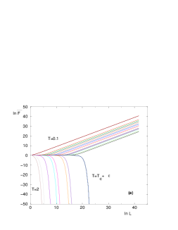
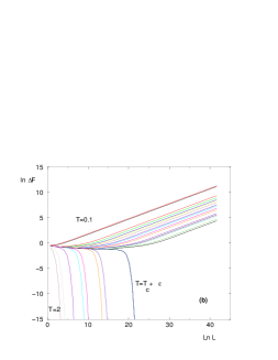
Figure 2: (Color online) Flows of the average value and of the width of the interface free-energy for many temperatures : (a) log-log plot of the average value $\overline{F}(L)$ of the free-energy distribution as a function of $L$. (b) log-log plot of the width $\Delta F(L)$ of the free-energy distribution as a function of $L$.

The flows of the average free-energy $\overline{F}(L)$ and of the free-energy width $\Delta F(L)$ are shown on Fig. 2 for many temperatures. One clearly sees on these log-log plots the two attractive fixed points separated by the critical temperature $T_{c}$. The value of $T_{c}$ obtained by the pool method depends on the pool, i.e. on the discrete sampling with $N$ values of the continuous probability distribution. It is expected to converge towards the thermodynamic critical temperature $T_{c}$ only in the limit $N\to\infty$. Nevertheless, for each given pool, the flow of free-energy allows a very precise determination of this pool-dependent critical temperature, for instance in the case considered $1.21685522<T_{c}^{pool}<1.21685523$.

For $T>T_{c}$, both the average free-energy and the free-energy width decay exponentially in $L$. For $T<T_{c}$, the average free-energy grows asymptotically with the interface dimension $d_{s}=d_{eff}-1=1$ (see Eq 11)

$$\overline{F}(L)\simeq\left(\frac{L}{\xi_{av}(T)}\right)^{d_{s}}+...\ \ \ {\rm with}\ \ d_{s}=1$$ (33)

where $\xi_{av}(T)$ is the correlation length that diverges as $T\to T_{c}^{-}$. The free-energy width grows asymptotically with the droplet exponent $\theta$ (see Eq 11)

$$\Delta F(L)\simeq\left(\frac{L}{\xi_{var}(T)}\right)^{\theta(b)}\ \ \ {\rm with}\ \ \theta(b=2)\simeq 0.299$$ (34)

where $\xi_{var}(T)$ is the associated correlation length that diverges as $T\to T_{c}^{-}$. Note that $\theta(b=2)\simeq 0.299$ is the droplet exponent of the corresponding directed polymer model [40, 39].

III.2 Divergence of the correlation lengths $\xi_{av}(T)$ and $\xi_{var}(T)$

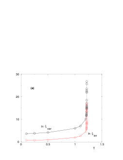
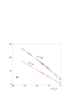
Figure 3: Divergence of the correlation lengths $\xi_{av}(T)$ $(\square)$ and $\xi_{var}(T)$ $(\bigcirc)$ (a) $\ln\xi_{av}(T)$ and $\ln\xi_{var}(T)$ as a function of $T$ (b) $\ln\xi_{av}(T)$ and $\ln\xi_{var}(T)$ as a function of $\ln|T_{c}-T|$ : the asymptotic slopes are of order $\nu_{av}\simeq 1.07$ and $\nu_{var}\simeq 1.34$

The correlation lengths $\xi_{av}(T)$ and $\xi_{var}(T)$ as measured from the free-energy average value (Eq 33) and from the free-energy width (Eq 34 ) are shown on Fig. 3 (a). The log-log plot shown on Fig. 3 (b) indicates power-law divergences with two distinct correlation length exponents

$$\xi_{av}(T) \mathop{\propto}_{T\to T_{c}}(T_{c}-T)^{-\nu_{av}}\ \ {\rm with}\ \ \nu_{av}\simeq 1.07$$

$$\xi_{var}(T) \mathop{\propto}_{T\to T_{c}}(T_{c}-T)^{-\nu_{var}}\ \ {\rm with}\ \ \nu_{var}\simeq 1.34$$ (35)

In conclusion, our numerical results point towards the following singular behavior for the interface free-energy (see Eq. 11)

$$F^{inter}(L,T<T_{c})\mathop{\propto}_{T\to T_{c}^{-}}\left(\frac{L}{\xi_{av}(T)}\right)^{d_{s}}+\left(\frac{L}{\xi_{var}(T)}\right)^{\theta}u_{F}+...$$ (36)

where the average contribution and the random contribution involve two correlation lengths $\xi_{av}(T)$ and $\xi_{var}(T)$ that diverge with distinct exponents (Eq 35). The presence of these two distinct correlation length exponents in the interface free-energy was a surprise for us, and we are not aware of any discussion of this possibility in the literature. The ’true’ correlation length is expected to be $\xi_{av}(T)$ that appears in the extensive non-random contribution to the interface free-energy. However, the presence of another length scale $\xi_{var}(T)$ that diverges with a larger exponent remains to be better understood.

III.3 Histogram of the interface free-energy below $T_{c}$

Figure 4: Statistics of the interface free-energy in the low-temperature phase (here $T=0.5$) : Log representation of the distribution $\Pi_{0}(x_{F})$ of the rescaled variable $x_{F}=\frac{F-\overline{F}}{\Delta F}$, which present asymmetric tails (see Eq. 38)

In the low-temperature phase, the the interface free-energy is expected to follow the behavior of Eq 11, where $u_{F}$ is a random behavior of order $O(1)$. We show on Fig. 4 the probability distribution $\Pi_{0}(x_{F})$ of the rescaled variable $x_{F}=\frac{F-\overline{F}}{\Delta F}$ in log-scale to see the tails. The two tails exponents $(\eta_{-},\eta_{+})$ defined by

$$\ln\Pi_{0}(x_{F})\mathop{\simeq}_{x_{F}\to\pm\infty}-|x_{F}|^{\eta_{\pm}}$$ (37)

are compatible with the relations proposed in our previous work [39] with $d_{s}=1$, $d=2$ and $\theta\simeq 0.299$ (see Eq 34)

$$\eta_{-} =\frac{d_{s}}{d_{s}-\theta}=\frac{1}{1-\theta}\sim 1.43$$

$$\eta_{+} =\frac{d}{d_{s}-\theta}=\frac{2}{1-\theta}\sim 2.85$$ (38)

III.4 Histogram of the interface free-energy at criticality

Figure 5: Histogram of the interface free-energy at criticality (a) Unrescaled probability distribution $P_{c}(F)$ of the interface free-energy $F$ at $T_{c}$ (b) Log representation of the distribution $\Pi_{c}(x_{F})$ of the rescaled variable $x_{F}=\frac{F-\overline{F}}{\Delta F}$

At criticality, the interface free-energy is expected to become a random variable of order $O(1)$ (Eq. 13) : we show its probability distribution on Fig. 5 (a). To see the tails, we show in log-scale the distribution of the rescaled variable $x_{F}=\frac{F-\overline{F}}{\Delta F}$ on Fig. 5 (b).

IV Statistics of the interface energy

In this section, we present the numerical results concerning the statistics of the interface energy.

IV.1 Average and width of the interface energy

As recalled in the introduction, the interface energy is expected to follow the scaling behavior of Eq 12 below $T_{c}$. The extensive non-random part $e_{0}(T)$ is directly related to the corresponding non-random part $f_{0}(T)$ of the free-energy of Eq. 11 via the usual thermodynamic relation

$$e_{0}(T)=f_{0}(T)-T\ \frac{df_{0}(T)}{dT}$$ (39)

As a consequence, the singularity found previously for $f_{0}(T)$ (Eq 33)

$$f_{0}(T)\simeq\left(\frac{1}{\xi_{av}(T)}\right)^{d_{s}}\mathop{\propto}_{T\to T_{c}^{-}}(T_{c}-T)^{d_{s}\nu_{av}}$$ (40)

determines the singularity of $e_{0}(T)$ near $T_{c}$

$$e_{0}(T)\mathop{\propto}_{T\to T_{c}^{-}}(T_{c}-T)^{d_{s}\nu_{av}-1}$$ (41)

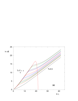
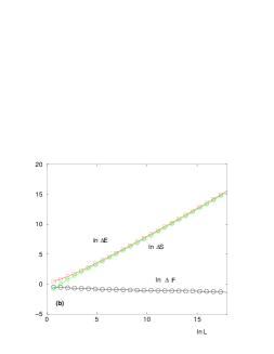
Figure 6: (Color online) Flow of the width $\Delta E(L)$ of the energy distribution as $L$ grows (a) $\ln\Delta E(L)$ as a function of $\ln L$ for many temperatures between $T=0.5$ and $T=T_{c}+\epsilon=1.21685523$ (b) Comparison of $\ln\Delta E(L)$ ($\square$), $\ln\Delta S(L)$ ($\Diamond$) and $\ln\Delta F(L)$ ($\bigcirc$) as a function of $\ln L$ at criticality.

We now consider the random contribution to the interface energy in Eq. 12. The flow of the width $\Delta E(L)$ as $L$ grows is shown on Fig. 6 for many temperatures. For $T<T_{c}$, this width grows asymptotically with the exponent $d_{s}/2=1/2$ as expected (see Eq 12)

$$\Delta E(L)\simeq L^{\frac{d_{s}}{2}}=L^{\frac{1}{2}}$$ (42)

Exactly at criticality, the energy width (and entropy width) grows as a power-law (see Fig 6 b)

$$\Delta E(L)\simeq L^{y_{c}}\ \ \ {\rm with}\ \ y_{c}\simeq 0.92$$ (43)

This value for $y_{c}$ is in agreement with the value $1/\nu_{av}\simeq 0.93$ (see Eq. 35).

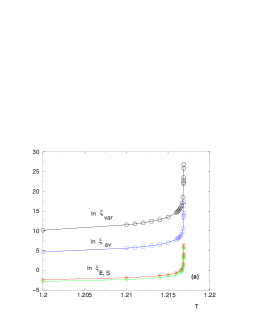
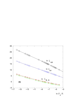
Figure 7: (Color online) Correlation lengths $\xi_{E}(T)$ ($\ast$) and $\xi_{S}(T)$ ($\Diamond$) as measured from the behavior of the energy and entropy widths (Eq. 45) (a) $\ln\xi_{E}(T)$ and $\ln\xi_{S}(T)$ as a function of $T$, as compared to $\ln\xi_{av}(T)$ ($\square$) and $\ln\xi_{var}(T)$ ($\bigcirc$) (b) $\ln\xi_{E}(T)$ and $\ln\xi_{S}(T)$ as a function of $\ln|T_{c}-T|$, as compared to $\ln\xi_{av}(T)$ and $\ln\xi_{var}(T)$

We now define a correlation length $\xi_{E}(T)$ for $T<T_{c}$ via the finite-size scaling form

$$\Delta E(L,T)\simeq L^{y_{c}}\Phi\left(\frac{L}{\xi_{E}(T)}\right)$$ (44)

In the regime $L\gg\xi_{E}(T)$, one should recover the $L$-dependence of the low-temperature phase of Eq 42, so the scaling function $\Phi(x)$ should present the asymptotic behavior $\Phi(x)\sim x^{1/2-y_{c}}$ yielding the temperature dependence of the prefactor

$$\Delta E(L,T)\mathop{\simeq}_{L\gg\xi_{E}(T)}\left(\frac{1}{\xi_{E}(T)}\right)^{1/2-y_{c}}L$$ (45)

One similarly may define a correlation length $\xi_{S}(T)$ from the finite-size scaling of the entropy width.

As shown on Fig 7 b, the log-log plot presents some curvature, so that the asymptotic slope $\nu_{E}$ defined by

$$\xi_{E}(T)\mathop{\simeq}(T_{c}-T)^{-\nu_{E}}$$ (46)

is difficult to measure precisely. However, the slope $\nu_{E}$ is close to the value $\nu_{av}\simeq 1.07$ of Eq. 35.

In conclusion, our numerical results point towards the following singular behavior for the interface energy (see Eq. 12)

$$E^{inter}(L,T<T_{c})\mathop{\propto}_{T\to T_{c}^{-}}\frac{1}{T_{c}-T}\left[\left(\frac{L}{\xi_{av}(T)}\right)^{d_{s}}+\left(\frac{L}{\xi_{av}(T)}\right)^{\frac{d_{s}}{2}}u_{E}+...\right]$$ (47)

i.e. both the average contribution and the random contribution involve the same correlation length $\xi_{av}(T)$. This result seems natural within the Fisher-Huse droplet theory [7, 13] where the interface energy is a sum of random terms that follow some Central Limit asymptotic behavior. This picture is confirmed by the Gaussian distribution of the random variable $u_{E}$ that we now consider.

IV.2 Histogram of the interface energy below $T_{c}$

Figure 8: Statistics of the interface energy in the low-temperature phase (here $T=0.5$) : Log representation of the distribution ${\tilde{\Pi}}_{0}(x_{E})$ of the rescaled variable $x_{E}=\frac{E-\overline{E}}{\Delta E}$ : it is a Gaussian

In the low-temperature phase, the the interface energy is expected to follow the behavior of Eq 12, where $u_{E}$ is a random variable of order $O(1)$ which is expected to be Gaussian distributed within the droplet theory [7, 13] : this is in agreement with our numerical histogram of the rescaled variable $x_{E}=\frac{E-\overline{E}}{\Delta E}$ shown on Fig 8.

IV.3 Histogram of the interface energy at criticality

Figure 9: Histogram of the interface energy at criticality (a) Unrescaled probability distribution $P_{n}(E)$ of the interface free-energy $E$ at $T_{c}$ at generation $n=22$ (b) Log representation of the distribution ${\tilde{\Pi}}_{c}(x_{E})$ of the rescaled variable $x_{E}=\frac{E-\overline{E}}{\Delta E}$

We show on Fig. 9 our numerical results for the histogram of the interface energy at criticality : the unrescaled distribution for $n=22$ generation is shown on Fig. 9 (a), whereas the distribution of the rescaled variable $x_{E}=\frac{E-\overline{E}}{\Delta E}$ is shown in log-scale on Fig. 9 (b). The fast decay of the tails show that the scaling of the interface energy at criticality is well measured via its variance (see Eq. 43).

V Statistics of the order parameter and of the interfacial adsorption

V.1 Statistics of the order parameter $M$

Below $T_{c}$, we find that the order parameter follows the scaling form

$$M(L,T<T_{c})\simeq m_{0}(T)L^{d}+m_{1}(T)L^{\frac{d}{2}}u_{i}$$ (48)

The coefficient $m_{0}(T)$ of the extensive non-random term vanishes at criticality with the exponent

$$m_{0}(T)\propto(T_{c}-T)^{\beta}\ \ {\rm with}\ \ \beta\simeq 0.163$$ (49)

Exactly at criticality, the order parameter is expected to follow the behavior of Eq. 8, up to a random variable $u_{c}$ of order $O(1)$

$$M(L,T_{c})\simeq L^{d-\frac{\beta}{\nu}}u_{c}$$ (50)

Our previous measures of $\nu_{av}\simeq 1.07$ (Eq. 35) and $\beta\simeq 0.163$ (Eq. 49) would correspond with $d=2$ to an exponent of order $d-\frac{\beta}{\nu_{av}}\simeq 1.85$. We measure (data not shown)

$$\overline{M}(L,T_{c})\sim\Delta M(L,T_{c})\sim L^{1.82}$$ (51)

in agreement with the scaling relation of Eq 50.

V.2 Statistics of the interfacial adsorption $N_{nb}$

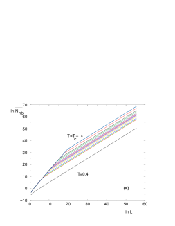
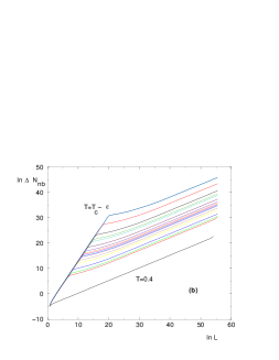
Figure 10: (Color online) Flows of the average value and of the width of the interfacial adsorption $N_{nb}$ for many temperatures : (a) log-log plot of the average value $\overline{N}_{nb}(L)$ as a function of $L$. (b) log-log plot of the width $\Delta N_{nb}(L)$ as a function of $L$.

The flows of the average value and of the width of the net absorption $N_{nb}$ of non-boundary states (defined in Eq 5) are shown on Fig. 10. Below $T_{c}$, we find the scaling form

$$N_{nb}(T<T_{c})\sim w_{0}(T)L^{d_{s}}+\delta(T)L^{\frac{d_{s}}{2}}v_{i}\ \ {\rm with}\ \ d_{s}=1$$ (52)

The coefficient $w_{0}(T)$ of the extensive non-random term is expected to diverge at criticality as in the pure case (Eq. 7). The coefficient $\delta(T)$ of the random term is expected to diverge to yield the same finite-size scaling as Eq. 8 exactly at criticality, so that

$$N_{nb}(L,T_{c})\sim L^{d-\frac{\beta}{\nu}}v_{c}$$ (53)

where $v_{c}$ is a random variable of order $O(1)$. We measure (see Fig. 10)

$$\overline{N}_{nb}(L,T_{c})\sim\Delta{N}_{nb}(L,T_{c})\sim L^{1.84}$$ (54)

again in agreement with the scaling relation of Eq 53.

The conclusion of this section is that our numerical results concerning the order parameter and the interfacial adsorption are consistent with ’conventional’ scaling in terms of the correlation length $\xi_{av}(T)$.

VI Comparison with the spin-glass on diamond lattice of effective dimension $d_{eff}=3$

The Migdal-Kadanoff renormalizations with a branching ratio $b=4$, which corresponds to an effective dimension $d_{eff}=3$ (Eq 18), have been much used to study spin-glasses [35, 36, 37, 38, 10, 11] (for the case $b=2$ corresponding to an effective dimension $d_{eff}=2$ there is no spin-glass phase). As recalled in the introduction, a new ’chaos exponent’ $\zeta_{c}>1/\nu$ has been introduced in [10, 11] to describe chaos properties at criticality, and this exponent was argued to govern the energy at criticality (Eq 17). In the following, we confirm this scenario by directly measuring the statistical properties of the interface energy. We also discuss the similarities and differences with the random ferromagnetic case discussed above.

VI.1 Flow of the width of the interface free-energy

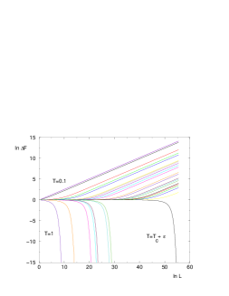
Figure 11: (Color online) Spin-glass transition : log-log plot of the width $\Delta F(L)$ of the free-energy distribution as a function of $L$, for many temperatures.

In the spin-glass case, there is no non-random leading term (Eq 9) in contrast to the random ferromagnetic case ( Eq 11). As a consequence, we only have to consider here the flow of the free-energy width $\Delta F(L)$ shown on Fig. 11. For $T>T_{c}$, the free-energy width decays exponentially in $L$. For $T<T_{c}$, the free-energy width grows asymptotically with the droplet exponent $\theta$ (see Eq. 9)

$$\Delta F(L)\simeq\left(\frac{L}{\xi_{var}(T)}\right)^{\theta(b)}\ \ \ {\rm with}\ \ \theta(b=4)\simeq 0.255$$ (55)

where $\xi_{var}(T)$ is the correlation length that diverges as $T\to T_{c}^{-}$. The exponent $\theta(b=4)\simeq 0.255$ is in agreement with previous measures [35, 38, 10].

Again, the critical temperature obtained by this pool method depends on the pool, i.e. on the discrete sampling with $N$ values of the continuous probability distribution. It is expected to converge towards the thermodynamic critical temperature $T_{c}$ only in the limit $N\to\infty$. Nevertheless, for each given pool, the flow of free-energy width allows a very precise determination of this pool-dependent critical temperature, for instance in the case considered $0.8810237<T_{c}^{pool}<0.88102375$. This value is in agreement with previous measures for a Gaussian initial condition [35, 38, 10].

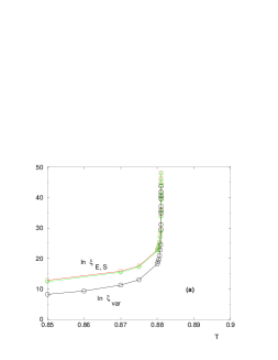
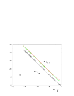
Figure 12: (Color online) Spin-glass transition : Correlation lengths $\xi_{var}(T)$ ($\bigcirc$), $\xi_{E}(T)$ ($\square$) and $\xi_{S}(T)$ ($\Diamond$) as measured from the behavior of the widths of the free-energy, energy and entropy distributions (a) $\ln\xi_{var}(T)$, $\ln\xi_{E}(T)$ and $\ln\xi_{S}(T)$ as a function of $T$ (b) $\ln\xi_{var}(T)$, $\ln\xi_{E}(T)$ and $\ln\xi_{S}(T)$ as a function of $\ln|T_{c}-T|$, : the asymptotic slope is the same and of order $\nu_{var}\simeq 2.92$

The correlation length $\xi_{var}(T)$ as measured from the free-energy width asymptotic behavior below $T_{c}$ (Eq 55 ) is shown on Fig. 12 (a). The plot in terms of the variable $\ln(T_{c}-T)$ shown on Fig. 12 (b) indicates a power-law divergence

$$\xi_{var}(T)\mathop{\propto}_{T\to T_{c}}(T_{c}-T)^{-\nu_{var}}\ \ {\rm with}\ \ \nu_{var}\simeq 2.92$$ (56)

VI.2 Flow of the width of the interface energy

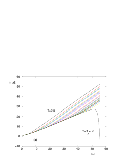
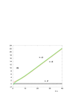
Figure 13: (Color online) Spin-glass transition : Flow of the width $\Delta E(L)$ of the energy distribution as $L$ grows (a) $\ln\Delta E(L)$ as a function of $\ln L$ for many temperatures between $T=0.5$ and $T=T_{c}+\epsilon=0.88102375$ (b) Comparison of $\ln\Delta E(L)$ , $\ln\Delta S(L)$ and $\ln\Delta F(L)$ as a function of $\ln L$ at criticality ($T_{c}^{pool}=0.8810237$).

The flow of the energy width $\Delta E(L)$ as $L$ grows are shown on Fig. 13 for many temperatures. For $T<T_{c}$, this width grows asymptotically with the exponent $d_{s}/2$ (see Eq. I.2)

$$\Delta E(L)\simeq L^{\frac{d_{s}}{2}}\simeq L\ \ \ {\rm with}\ \ d_{s}(b=4)=d_{eff}(b=4)-1=2$$ (57)

Exactly at criticality, the energy width (and entropy width) grows as a power-law (see Fig 13 b)

$$\Delta E(L,T_{c})\simeq L^{\zeta_{c}}\ \ \ {\rm with}\ \ \zeta_{c}\simeq 0.58$$ (58)

This exponent is clearly greater than $1/\nu_{var}\simeq 0.34$ (see Eqs 56) and coincides with the chaos critical exponent measured in [10].

We now define a correlation length $\xi_{E}(T)$ for $T<T_{c}$ via the finite-size scaling form

$$\Delta E(L,T)\simeq L^{\zeta_{c}}\Phi\left(\frac{L}{\xi_{E}(T)}\right)$$ (59)

In the regime $L\gg\xi_{E}(T)$, one should recover the $L$-dependence of the low-temperature phase of Eq 57, so the scaling function $\Phi(x)$ should present the asymptotic behavior $\Phi(x)\sim x^{1-\zeta_{c}}$ yielding the temperature dependence of the prefactor

$$\Delta E(L,T)\mathop{\simeq}_{L\gg\xi_{E}(T)}\left(\frac{1}{\xi_{E}(T)}\right)^{1-\zeta_{c}}L$$ (60)

As shown on Fig 12, this leads to the same divergence as in Eq 56

$$\xi_{E}(T)\mathop{\simeq}(T_{c}-T)^{-\nu_{var}}\ \ \ {\rm with}\ \ \nu_{var}\simeq 2.95$$ (61)

VII Summary and conclusions

In this paper, we have studied the statistical properties of critical system-size interfaces in a disordered Potts ferromagnet. For the interface free-energy, our numerical results point towards the following singular behavior for the interface free-energy

$$F^{inter}(L,T<T_{c}) \simeq f_{0}(T)L^{d_{s}}+\Upsilon(T)L^{\theta}u_{F}+...$$ (62)

$$\mathop{\propto}_{T\to T_{c}^{-}}\left(\frac{L}{\xi_{av}(T)}\right)^{d_{s}}+\left(\frac{L}{\xi_{var}(T)}\right)^{\theta}u_{F}(T,L)+...$$

where the average contribution and the random contribution involve two correlation lengths $\xi_{av}(T)$ and $\xi_{var}(T)$ that diverge with distinct exponents at criticality (Eq 35). The ’true’ correlation length is expected to be $\xi_{av}(T)$ that appears in the extensive non-random contribution to the interface free-energy. In particular, we have found that the interface energy follows the scaling form

$$E^{inter}(L,T<T_{c})\mathop{\propto}_{T\to T_{c}^{-}}\frac{1}{T_{c}-T}\left[\left(\frac{L}{\xi_{av}(T)}\right)^{d_{s}}+\left(\frac{L}{\xi_{av}(T)}\right)^{\frac{d_{s}}{2}}u_{E}+...\right]$$ (63)

i.e. both the average contribution and the random contribution involve the same correlation length $\xi_{av}(T)$. This result seems natural within the Fisher-Huse droplet theory [7, 13] where the interface energy is a sum of random terms that follow some Central Limit asymptotic behavior. This picture is confirmed by the Gaussian distribution of the random variable $u_{E}$, and by the ’conventional’ behavior exactly at criticality

$$E^{inter}(L,T_{c})\sim L^{\frac{1}{\nu_{av}}}u_{E_{c}}$$ (64)

However, the presence of another length scale $\xi_{var}(T)$ that diverges with a greater exponent $\nu_{var}>\nu_{av}$ remains to be better understood, in particular if one compares with the spin-glass transition. In the spin-glass case, $\xi_{var}(T)$ appearing in the random contribution of the free-energy is considered as the ’true’ correlation length, since this is the leading term in the free-energy in this case. But then the interface energy is governed by some critical chaos exponent $E^{inter}(L,T_{c})\sim L^{\zeta_{c}}$ exactly at criticality, with $\zeta_{c}>1/\nu_{var}$, in contrast with the ’conventional’ behavior of Eq. 64. So in both cases, even if the physical interpretation is different, one needs two different diverging length scales to describe the critical behaviors of the random contributions of the free-energy and energy or entropy. The physical origin seems to be in the chaos property of the random variable $u_{F}(T,L)$ of order $O(1)$ in Eq. 62. Within one disordered sample, the random variable $u_{F}(T,L)$ strongly depends on the temperature, and this is why the energy and the entropy of the interface presents fluctuations that are not directly related to the scalings appearing in the free-energy. More precisely, the entropy can be obtained as a derivative of the free-energy with respect to temperature

$$S^{inter}(L,T<T_{c}) =-\frac{dF^{inter}(L,T)}{dT}$$ (66)

$$=-\frac{df_{0}(T)}{dT}L^{d_{s}}-\frac{d\Upsilon(T)}{dT}L^{\theta}u_{F}(T,L)-\Upsilon(T)L^{\theta}\frac{\partial u_{F}(T,L)}{\partial T}$$

(and similarly the energy reads $E^{inter}=F^{inter}-T\frac{dF^{inter}}{dT}$). The first term is the extensive term, the second term is only of order $L^{\theta}$, and thus we conclude that the fluctuation term of order $\sigma(T)L^{d_{s}/2}$ with $d_{s}=d-1$ present in the entropy and in the energy ( Eq. 12) has for origin the derivative of the random variable $u_{F}(T,L)$. The identification of these two terms yields

$$\Upsilon(T)L^{\theta}\frac{\partial u_{F}(T,L)}{\partial T}\sim\sigma(T)L^{\frac{d_{s}}{2}}u_{E}$$ (67)

i.e. the derivative

$$T\frac{\partial u_{F}(T,L)}{\partial T}\sim\frac{\sigma(T)}{\Upsilon(T)}L^{\frac{d_{s}}{2}-\theta}u_{E}\sim\frac{\sigma(T)}{\Upsilon(T)}L^{\zeta}u_{E}$$ (68)

is of order $L^{\zeta}$ where $\zeta=\frac{d_{s}}{2}-\theta$ is the chaos exponent of the zero-temperature fixed point. Let us now consider the singularity of the prefactor $\frac{\sigma(T)}{\Upsilon(T)}$ as $T\to T_{c}$. If one defines a chaos length $L_{ch}(T)$ via

$$\frac{\sigma(T)}{\Upsilon(T)}L^{\zeta}\sim\frac{1}{(T_{c}-T)}\left(\frac{L}{L_{ch}(T)}\right)^{\zeta}$$ (69)

one obtains that this chaos length $L_{ch}(T)$ diverges more slowly than the correlation length. More precisely, in the random ferromagnetic case, using $\Upsilon(T)\sim 1/(\xi_{var}(T))^{\theta}$ and $\sigma(T)\sim 1/((T_{c}-T)\xi_{av}^{d_{s}/2}(T))$, one obtains the singularity

$${\rm Random\ Ferromagnets:}\ \ L_{ch}(T)=\xi_{av}(T)\times\left(\frac{\xi_{var}(T)}{\xi_{av}(T)}\right)^{-\frac{\theta}{\zeta}}$$ (70)

So here the difference in scaling between the chaos length $L_{ch}(T)$ and the correlation length $\xi_{av}(T)$ comes from the difference between $\xi_{var}(T)$ and $\xi_{av}(T)$. In the spin-glass case, using $\Upsilon(T)\sim 1/(\xi_{var}(T))^{\theta}$ and $\sigma(T)\sim(\xi_{var}(T))^{\zeta_{c}-d_{s}/2}$, one obtains the singularity

$${\rm Spin\ Glass:}\ \ L_{ch}(T)=\xi_{var}(T)\times(\xi_{var}(T))^{-\frac{\zeta_{c}-\frac{1}{\nu_{var}}}{\zeta}}$$ (71)

Here, the difference in scaling between the chaos length $L_{ch}(T)$ and the correlation length $\xi_{av}(T)$ comes from the difference $\zeta_{c}-\frac{1}{\nu_{var}}>0$.

In conclusion, beyond the differences in interpretation concerning the nature of the transition in disordered ferromagnets (where the ’true’ correlation length is $\xi_{av}(T)$ associated to the non-random term of the free-energy, and where the interface energy presents conventional scaling at criticality $E(L,T_{c})\sim L^{1/\nu_{av}}$) and in spin-glasses (where the ’true’ correlation length is $\xi_{var}(T)$ associated to the random term of the free-energy, and where the interface energy presents non-conventional scaling at criticality $E(L,T_{c})\sim L^{\zeta_{c}}$ with a critical chaos exponent $\zeta_{c}>1/\nu_{var}$), the common feature seems to be that in both cases, the characteristic length scale $L_{ch}(T)$ associated with the chaotic nature of the low-temperature phase, diverges more slowly than the correlation length. Note that for spin-glasses, Nifle and Hilhorst have found that the inequality $\zeta_{c}>1/\nu$ is satisfied in a finite range of dimensions $d_{-}<d<d_{+}$ above the lower critical dimension $d_{-}$ , whereas for $d>d_{+}$, the usual scaling laws in terms of the correlation length exponent $\nu$ are valid [10]. In disordered ferromagnets, one may similarly wonder whether the different singularities in $\xi_{av}(T)$ and $\xi_{var}(T)$ exist only in a finite range of dimensions $d_{-}<d<d_{+}$. It would be nice to clarify in which conditions the critical point of a disordered model is described by a single diverging length scale or by two diverging length scales. This probably requires a more precise understanding of the geometrical properties of the interface in the critical region that should be different for $d<d_{+}$ and $d>d_{+}$.

Appendix A Reminder on the pure Potts model on hierarchical lattices

In the pure case, the renormalization of Eq. 23 reduces to the mapping $T$ discussed in [33, 41]

$$x_{n+1}=T(x_{n})=\left(\frac{x_{n}^{2}+(q-1)}{2x_{n}+(q-2)}\right)^{b}=T(x_{n})$$ (72)

The two attractive fixed points $x=1$ (infinite temperature) and $x=\infty$ (zero temperature) are separated by a repulsive fixed point $x_{c}$ (critical point). The critical exponents are obtained as follows [33, 41] : the critical exponent $\nu$ is determined by the linearized mapping around the critical point

$$\nu=\frac{\ln 2}{\ln T^{\prime}(x_{c})}$$ (73)

and the specific heat exponent reads

$$\alpha=2-d_{eff}\nu=2-\frac{\ln(2b)}{\ln T^{\prime}(x_{c})}$$ (74)

where $d_{eff}=(\ln(2b)/\ln(2)$ represents the dimension of the hierarchical lattice. In addition to usual power-laws, there are logarithmic oscillations coming from the discrete nature of the renormalization [41]. For $b=2$ (effective dimension $d_{eff}=2$), the critical point $x_{c}(q)$ corresponds to

$$q=(x_{c}-1)(\sqrt{x}_{c}-1)$$ (75)

and the transition is second order for any $q$. The Harris criterion indicates that disorder is relevant for

$$q>q_{Harris}(b=2)=4+2\sqrt{2}\sim 6.828...$$ (76)

and this is why we have chosen to use the value $q=8$ for our numerical simulations of the disordered case.

References

- [1] B. Widom, ”Phase transitions and critical phenomena’, Domb and Green Eds, vol. 2, page 79 (NY academic press 1972).
- [2] O. Schramm, Israel J. Math. 118, 221 (2000).
- [3] W. Werner, arXiv:math/0303354; J. Cardy, Ann. Phys. NY 318, 81 (2005); M. Bauer and D. Bernard, Phys. Rep. 432, 115 (2006).
- [4] A. Gamsa and J. Cardy, J. Stat. Mech. P12009 (2005).
- [5] M. Picco and R. Santachiara, arXiv:0708.4295.
- [6] W. Selke and W. Resch, Z. Phys. B 47, 335 (1982); W. Selke and D.A. Huse, Z. Phys. B 50, 113 (1983); W. Selke, D.A. Huse and D.M. Kroll, J. Phys. A 17, 3019 (1984); J. Yeomans and B. Derrida, J. Phys. A 18, 2343 (1985).
- [7] D.S. Fisher and D.A. Huse, Phys. Rev. Lett. 56, 1601 (1986); D.S. Fisher and D.A. Huse, Phys. Rev. B38, 386 (1988).
- [8] A.J. Bray and M. A. Moore, in Heidelberg colloquium on glassy dynamics, J.L. van Hemmen and I. Morgenstern, Eds (Springer Verlag, Heidelberg, 1986).
- [9] J.R. Banavar and A.J. Bray, Phys. Rev. B 35, 8888 (1987); T. Aspelmeier, A.J. Bray and M.A. Moore, Phys. Rev. Lett. 89, 197202 (2002).
- [10] M. Nifle and H.J. Hilhorst, Phys. Rev. Lett. 68 (1992) 2992 ; M. Ney-Nifle and H.J. Hilhorst, Physica A 193 (1993) 48; M. Ney-Nifle and H.J. Hilhorst, Physica A 194 (1993) 462; M. Ney-Nifle, Phys. Rev. B 57, 492 (1998).
- [11] M.J. Thill and H.J. Hilhorst, J. Phys. I France 6, 67 (1996)
- [12] D. A. Huse, C. L. Henley, Phys. Rev. Lett. 54, 2708 (1985).
- [13] D.S. Fisher and D.A. Huse, Phys. Rev. B43, 10728 (1991).
- [14] D. A. Huse, C. L. Henley, and D. S. Fisher, Phys. Rev. Lett. 55, 2924 (1985).
- [15] M. Kardar, Nucl. Phys. B 290 582 (1987).
- [16] K. Johansson, Comm. Math. Phys. 209 (2000) 437.
- [17] X.H. Wang, S. Havlin and M. Schwartz, Phys. Rev. E 63 (2001) 032601; X.H. Wang, S. Havlin and M. Schwartz, J. Phys. Chem. B 104 (2000) 3875.
- [18] Y.C. Zhang, Phys. Rev. Lett. 59 2125 (1987); T.Nattermann, Phys. Rev. Lett. 60 , 2701 (1988).
- [19] M.V. Feigelman and V.M. Vinokur, Phys. Rev. Lett. 61 (1988) 1139.
- [20] Y. Shapir, Phys. Rev. Lett. 66, 1473 (1991).
- [21] C. Monthus and T. Garel, arXiv:0710.0735.
- [22] C. Amoruso, A.K. Hartmann, M.B. Hastings and M.A. Moore, Phys. Rev. Lett. 97, 267202 (2006); D. Bernard, P. Le Doussal and A.A. Middleton, Phys. Rev. B76, 020403(R) (2007).
- [23] S. Risau-Gusman, F. Roma, arXiv:0711.0205.
- [24] S. Wiseman and E. Domany, Phys. Rev. E 52, 3469 (1995); A. Aharony and A.B. Harris, Phys. Rev. Lett. 77, 3700 (1996); S. Wiseman and E. Domany, Phys. Rev. Lett. 81, 22 (1998); S. Wiseman and E. Domany, Phys. Rev. E 58, 2938 (1998).
- [25] M. Kardar, A.L. Stella, G. Sartoni and B. Derrida, Phys. Rev. E 52, R1269 (1995).
- [26] J. Cardy, Nucl. Phys. B 565, 506 (2000).
- [27] Th. Niemeijer, J.M.J. van Leeuwen, ”Renormalization theories for Ising spin systems” in Domb and Green Eds, ”Phase Transitions and Critical Phenomena” (1976); T.W. Burkhardt and J.M.J. van Leeuwen, “Real-space renormalizations”, Topics in current Physics, Vol. 30, Spinger, Berlin (1982); B. Hu, Phys. Rep. 91, 233 (1982).
- [28] A.A. Migdal, Sov. Phys. JETP 42, 743 (1976) ; L.P. Kadanoff, Ann. Phys. 100, 359 (1976).
- [29] A.N. Berker and S. Ostlund, J. Phys. C 12, 4961 (1979).
- [30] M. Kaufman and R. B. Griffiths, Phys. Rev. B 24, 496 - 498 (1981); R. B. Griffiths and M. Kaufman, Phys. Rev. B 26, 5022 (1982).
- [31] C. Jayaprakash, E. K. Riedel and M. Wortis, Phys. Rev. B 18, 2244 (1978)
- [32] W. Kinzel and E. Domany, Phys. Rev. B 23, 3421 (1981).
- [33] B. Derrida and E. Gardner, J. Phys. A 17, 3223 (1984); B. Derrida in ”Critical phenomena, random systems , gauge theories”, Les Houches 1984, K. Osterwalder and R. Stora (Eds), North Holland (1986), page 989.
- [34] D. Andelman and A.N. Berker, Phys. Rev. B 29, 2630 (1984).
- [35] A. P. Young and R. B. Stinchcombe, J. Phys. C 9 (1976) 4419 ; B. W. Southern and A. P. Young J. Phys. C 10 ( 1977) 2179.
- [36] S.R. McKay, A.N. Berker and S. Kirkpatrick, Phys. Rev. Lett. 48 (1982) 767; E. J. Hartford and S.R. McKay, J. Appl. Phys. 70, 6068 (1991).
- [37] E. Gardner, J. Physique 45, 115 (1984).
- [38] A.J. Bray and M. A. Moore, J. Phys. C 17 (1984) L463; J.R. Banavar and A.J. Bray, Phys. Rev. B 35, 8888 (1987); M. A. Moore, H. Bokil, B. Drossel Phys. Rev. Lett. 81 (1998) 4252; S. Boettcher, Eur. Phys. J. B 33, 439 (2003).
- [39] C. Monthus and T. Garel, arXiv:0710.2198
- [40] B. Derrida and R.B. Griffiths, Europhys. Lett. 8 , 111 (1989).
- [41] B. Derrida, C. Itzykson and J.M. Luck, Comm. Math. Phys. 94, 115 (1984).