Trellis Computations

Abstract

For a certain class of functions, the distribution of the function values can be calculated in the trellis or a sub-trellis. The forward/backward recursion known from the BCJR algorithm [1] is generalized to compute the moments of these distributions. In analogy to the symbol probabilities, by introducing a constraint at a certain depth in the trellis we obtain symbol moments. These moments are required for an efficient implementation of the discriminated belief propagation algorithm in [2], and can furthermore be utilized to compute conditional entropies in the trellis.

The moment computation algorithm has the same asymptotic complexity as the BCJR algorithm. It is applicable to any commutative semi-ring, thus actually providing a generalization of the Viterbi algorithm [3].

I Introduction

Trellises were introduced into the coding theory literature by Forney [4] as a means of describing the Viterbi algorithm for decoding convolutional codes. Bahl et al. [1] showed that block codes can also be described by a trellis, and Wolf [5] proposed the use of the Viterbi algorithm for trellis-based soft-decision decoding of block codes. Massey [6] gave a graph-theoretic definition of a block trellis and an alternative construction of minimal trellises. Forney’s paper [7] showed that group codes, including linear codes and lattices, have a well-defined trellis structure.

In [8], McEliece investigated the complexity of a generalized Viterbi algorithm which allows efficient computation of flows on a code trellis. These results were further generalized in [9] and [10]. However, the calculation of flows does not fully exploit the capabilities of the trellis (representation): For a certain set of functions it is possible to calculate the moments of these functions in the trellis. These can be scalar or vectorial, as long as they are linear and fulfill a separability criterion.

For iterative decoding of coupled codes, the popular sum-product algorithm is used to calculate the symbol probabilities of the component codes. These probabilities are exchanged between component decoders until a stable solution is found. This iterative algorithm works very well for long “turbo”, low-density parity check (LDPC) and some other codes, obtained by concatenation of simple component codes in a special way. However, performance becomes poor when utilizing short or some good component codes.

Recently, Sorger [2] showed that iterative decoding is improved when discriminating code words $\mathbf{c}$ by their correlation $\mathbf{c}\mathbf{r}^{T}$ or $\mathbf{c}\mathbf{w}^{T}$ with the received word $\mathbf{r}$ or a ‘believed’ word $\mathbf{w}$, respectively. Not only symbol probabilities are considered, but also the distribution of these probabilities over the correlation value. An efficient algorithm is introduced using the first two moments to approximate these distributions.

In this paper we propose algorithms to compute both such distributions and their moments in the trellis.

Example 1

Consider Figure 1

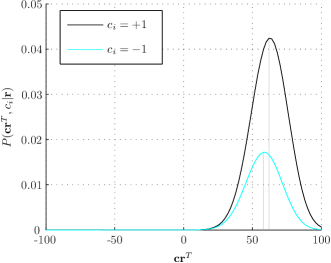
Figure 1: Symbol Distributions of Correlation $\mathbf{cr}^{T}$

which shows two distributions of the correlation function $\mathbf{c}\mathbf{r}^{T}$, where $\mathbf{c}$ is a code word and $\mathbf{r}$ is the noisy version of a code word $\check{\mathbf{c}}\in\mathbb{C}$ after transmission over a memory-less binary symmetric channel (BSC). The curves show the distributions for $\mathbf{c}\in\mathbb{C}_{i}(+1)$ and $\mathbf{c}\in\mathbb{C}_{i}(-1)$, respectively, where $\mathbb{C}_{i}(x):=\left\{\mathbf{c}\in\mathbb{C}:c_{i}=x\right\}$ denotes the sub-code of $\mathbb{C}$ for which the symbol $c_{i}$ at a given position $i$ of each code word equals $x\in\{-1,+1\}$. The integrals over the distributions equal the symbol probabilities $P(c_{i}=x|\mathbf{r})$. However, the probability ratio

$$\frac{P(\mathbf{c}\mathbf{r}^{T},c_{i}=+1|\mathbf{r})}{P(\mathbf{c}\mathbf{r}^{T},c_{i}=-1|\mathbf{r})}$$ (1)

varies significantly over $\mathbf{cr}^{T}$ which can be exploited when knowledge on the correlation $\check{\mathbf{c}}\mathbf{r}^{T}$ with the transmitted code word is available.

The distributions in Figure 1 can be approximated with their moments

$$\mathrm{E}_{\mathbf{C}}\left[\left.\left(\mathbf{cr}^{T}\right)^{m}\right|\mathbf{r},c_{i}\right]:=\sum_{\mathbf{c}\in\mathbb{C}}\left(\mathbf{cr}^{T}\right)^{m}\cdot P(\mathbf{c}|\mathbf{r},c_{i})$$ (2)

up to a certain order $m$, where $\mathrm{E}_{\mathbf{C}}[.]$ is the expectation over all code words $\mathbf{c}\in\mathbb{C}$. The distributions will be Gaussian for sufficiently long codes which can be understood by the law of large numbers. Hence we can expect the first two moments to suffice for a good approximation.

We present generalizations of the methods in [8] which enable us to compute distributions $P(\mathbf{c}\mathbf{w}^{T},c_{i}=+1|\mathbf{r})$ and expressions like $\mathrm{E}_{\mathbf{C}}\left[\left(\mathbf{cw}^{T}\right)^{m}|\mathbf{r},c_{i}\right]$ for some word $\mathbf{w}$, whereof (2) is a special case, both for hard and soft decision. The complexity of the algorithm is of the same order as the classically used BCJR algorithm.

The remainder of this paper is structured as follows. The next section contains a review of common terminology in the context of trellises. This is extended in Section III, which deals with the computation of distributions and their moments in a more general frame. In Section IV we will return to the original problem by transferring the results of Section III to linear block codes and calculate the conditional entropy in the trellis.

II Definitions

We deliberately follow to a wide extent the notation and style of McEliece. The first paragraph is an excerpt from [8] with minor modifications.

A trellis $T=(\mathbb{V},\mathbb{E})$ of rank $n$ is a finite-directed graph with vertex set $\mathbb{V}$ and edge set $\mathbb{E}$, in which every vertex is assigned a depth in the range $\{0,1,\dots,n\}$. Each edge is connecting a vertex at depth $i-1$ to one at depth $i$, for some $i\in\{0,1,\dots,n\}$. Multiple edges between vertices are allowed. The set of vertices at depth $i$ is denoted by $\mathbb{V}_{i}$, so that $\mathbb{V}=\bigcup_{i=0}^{n}\mathbb{V}_{i}$. For $v\in\mathbb{V}_{i}$ we write $\mathrm{depth}(v)=i$. The set of edges connecting vertices at depth $i-1$ to those at depth $i$ is denoted $\mathbb{E}_{i-1,i},$ so that $\mathbb{E}=\bigcup_{i=1}^{n}\mathbb{E}_{i-1,i}$. There is only one vertex at depth $0$, called $A$, and only one at depth $n$, called $B$. If $e\in\mathbb{E}$ is a directed edge connecting the vertices $u$ and $v$, which we denote by $e:u\rightarrow v$, we call $u$ the initial vertex, and $v$ the final vertex of $e$ and write $\mathrm{init}(e)=u$, $\mathrm{fin(e})=v$. We denote the number of edges leaving a vertex $v$ by $\rho^{+}(v)$, and the number of edges entering a vertex $v$ by $\rho^{-}(v)$, i.e.

$$\rho^{+}(v) = |\{e:\mathrm{init}(e)=v\}|$$

$$\rho^{-}(v) = |\{e:\mathrm{fin}(e)=v\}|.$$

If $u$ and $v$ are vertices, a path $\mathtt{P}$ of length $L$ from $u$ to $v$ is a sequence of $L$ edges: $\mathtt{P}=e_{1}e_{2}\cdots e_{L}$, such that $\mathrm{init}(e_{1})=u$, $\mathrm{fin}(e_{L})=v$, and $\mathrm{fin}(e_{i})=\mathrm{init}(e_{i+1})$, for $i=1,2,\dots,L-1$. If $\mathtt{P}$ is such a path, we sometimes write $\mathtt{P}:u\rightarrow v$ for short, as well as $\mathrm{init}(\mathtt{P})=\mathrm{init}(e_{1})$ and $\mathrm{fin}(\mathtt{P})=\mathrm{fin}(e_{L})$. We denote the set of paths from vertices at depth $i$ to vertices at depth $j$ by $\mathbb{E}_{i,j}$. We assume that for every vertex $v\neq A,B$, there is at least one path from $A$ to $v$, and at least one path from $v$ to $B$.

Example 2 (Trellis)

Figure 2

Figure 2: Trellis of rank $n=4$ with vertex set $\mathbb{V}=\{A,1,2,3,4,5,6,B\}$ and edge set $\mathbb{E}=\{\mathtt{a},\mathtt{b},\mathtt{c},\mathtt{d},\mathtt{e},\mathtt{f},\mathtt{g},\mathtt{h},\mathtt{i},\mathtt{j},\mathtt{k},\mathtt{l}\}$

shows a trellis of rank $n=4$ with edge set $\mathbb{E}=\{\mathtt{a},\mathtt{b},\mathtt{c},\mathtt{d},\mathtt{e},\mathtt{f},\mathtt{g},\mathtt{h},\mathtt{i},\mathtt{j},\mathtt{k},\mathtt{l}\}$ and vertex set $\mathbb{V}=\{A,1,2,3,4,5,6,B\}$. There are eight paths $\mathtt{P}:A\rightarrow B$ from $A$ to $B$. There is $\rho^{-}(1)=1$ edge entering (edge $\mathtt{a}$) and $\rho^{+}(1)=2$ edges (edges $\mathtt{c}$ and $\mathtt{d}$) leaving vertex $v=1$.

We assume each edge in the trellis is labeled. Let $T=(\mathbb{V},\mathbb{E})$ be a trellis of rank $n$, such that each edge $e\in\mathbb{E}$ is labeled with a real valued number $\lambda(e)\in\mathbb{R}$. We now define the label of a path, and the flow between two vertices.

Definition 1 (Path Labels)

The label $\lambda(\mathtt{P})$ of a path $\mathtt{P}=e_{1}e_{2}\cdots e_{L}$ is defined as the product $\lambda(\mathtt{P})=\lambda(e_{1})\cdot\lambda(e_{2})\cdot\dots\,\cdot\lambda(e_{L})$ of the labels of all edges in the path. (Note that the subscript indicates the sequence number rather than the edge’s depth.)

Definition 2 (Flow)

If $u$ and $v$ are vertices in a labeled trellis, we define the flow $\eta(u,v)$ from $u$ to $v$ to be the sum of the labels on all paths from $u$ to $v$, i.e.,

$$\eta(u,v)=\sum_{\mathtt{P}:u\rightarrow v}\lambda(\mathtt{P})\,.$$

In this paper, we only consider operations on the set of real numbers with ordinary addition and multiplication as the authors are not aware of application for other algebraic structures. However, Appendix -C briefly shows that the algorithm can be transferred to any commutative semi-ring, thus leading to a generalization of the Viterbi algorithm [3].

Example 3

We continue Example 2. The trellis depicted in Figure 2 is the trellis of the $(4,3,2)$ single parity check code. In the BCJR algorithm, the edge labels $\lambda(e)$ are the channel probabilities of the corresponding transitions.

III Trellis-Based Computations

In this section we consider distributions of the type

$$\mathcal{D}:\,q\mapsto D(q)=\sum_{{\mathtt{P}:A\rightarrow B\atop f(\mathtt{P})=q}}\lambda\left(\mathtt{P}\right)$$

for special functions $f$, i.e., $q$ is mapped to the sum of the labels of all paths $\mathtt{P}$ with $f(\mathtt{P})=q$. We present an algorithm to calculate these distributions over all paths of a trellis or a sub-set of these. Before, however, we develop algorithms to calculate the moments

$$\bar{\theta}^{(m)}(T):=\frac{\sum_{\mathtt{P}}\left(f(\mathtt{P})\right)^{m}\cdot\lambda(\mathtt{P})}{\sum_{\mathtt{P}}\lambda(\mathtt{P})}$$

and - by introducing a constraint on the paths - the symbol moments

$$\bar{\Omega}^{(m)}_{i}(T,x):=\frac{{\displaystyle\sum_{{\mathtt{P}:A\rightarrow B\atop c(e_{i})=x}}}\left(f(\mathtt{P})\right)^{m}\cdot\lambda(\mathtt{P})}{{\displaystyle\sum_{{\mathtt{P}:A\rightarrow B\atop c(e_{i})=x}}}\lambda(\mathtt{P})}$$

of such distributions in the trellis. We show that the complexity of the moment calculation algorithm is $O(|\mathbb{E}|)$, where $|\mathbb{E}|$ is the number of edges in the trellis.

To each edge $e\in\mathbb{E}$ of the trellis $T$ we introduce a second label $c(e)\in\mathbb{R}$, which we will refer to as the c-label. For distinction, we will call $\lambda(e)$ the $\lambda$-label.

Example 4

We continue Example 3. Solid lines correspond to the c-label $c(e)=1$, dashed lines correspond to $c(e)=-1$ (bipolar binary notation). E.g., the path $\mathtt{P}=\mathtt{a}\mathtt{d}\mathtt{i}\mathtt{k}$ has the c-label $\mathbf{c}(\mathtt{P})=+1\,-1\,-1\,+1$ which is a code word.

Let

$$g_{i}\left(c(e)\right):x\mapsto y;\,x,y\in\mathbb{R}$$

be a common function of $c(e)$ for all edges $e\in\mathbb{E}_{i-1,i}$. Further, let

$$f\left(\mathbf{c}(\mathtt{P})\right)=f\left(c(e_{1}),c(e_{2}),\dots,c(e_{L})\right):\mathbf{c}\mapsto y;\,c(e_{i}),y\in\mathbb{R}$$

be a function of the c-labels of the edges of a path $\mathtt{P}$ with length $L$. The bold letter indicates that $\mathbf{c}$ is a vector. For simplicity, in the following we will abbreviate $g_{i}\left(c(e)\right)$ and $f\left(\mathbf{c}(\mathtt{P})\right)$ by $g_{i}(e)$ and $f(\mathtt{P})$, respectively. The functions $f(\mathtt{P})$ have to fulfill the linearity criterion

$$f(\mathtt{P})=f(e_{1}e_{2}\cdots e_{n})=g_{1}(e_{1})+g_{2}(e_{2})+\dots+g_{n}(e_{n})$$ (3)

for all paths $\mathtt{P}:A\rightarrow B$.

Definition 3 (Forward Numerator)

We define the $m$-th forward numerator of a function $f$ at vertex $v$ of a trellis $T$ as

$$\alpha^{(m)}(v):=\sum_{\mathtt{P}:A\rightarrow v}\left(f(\mathtt{P})\right)^{m}\cdot\lambda(\mathtt{P})$$ (4)

with initial values

$$\alpha^{(m)}(A):=\left\{\begin{array}[]{ccc}1&:&m=0\\ 0&:&m>0\end{array}\right.\;.$$

Theorem 1 (Forward Recursion)

The $m$-th forward numerator $\alpha^{(m)}(v)$ of a vertex $v\in V_{i}$ on depth $i$ can be recursively calculated on a trellis $T$ by

$$\alpha^{(m)}(v)=\sum_{e:\mathrm{fin}(e)=v}\lambda(e)\cdot\sum_{l=0}^{m}{m\choose l}\left(g_{i}(e)\right)^{l}\cdot\alpha^{(m-l)}\left(\mathrm{init}(e)\right)$$ (5)

as in Algorithm 1.

Algorithm 1 Computation of first ($M$+1) Forward Numerators

01: /* initialization */

02: $\alpha^{(0)}(A)=1;$

03: for (m=1 to m_max)

04:   $\alpha^{(m)}(A)=0$;

05: /* recursion */

06: for (i=1 to n) {

07:  for ($v\in\mathbb{V}_{i}$) {

08:   for (m=0 to m_max)

09:    $\alpha^{(m)}(v)={\displaystyle\sum_{e:\mathrm{fin}(e)=v}}\lambda(e)\cdot{\displaystyle\sum_{l=0}^{m}}{m\choose l}\left(g_{i}(e)\right)^{l}\cdot$

$\hskip 179.25235pt\cdot\alpha^{(m-l)}\left(\mathrm{init}(e)\right);$

10:   }

11:  }

12: }

Proof:

The proof is by induction on $\mathrm{depth}(v)$. For $\mathrm{depth}(v)=1$, it follows from the definition of a trellis that all paths from $A$ to $v$ must consist of just one edge $e$, with $\mathrm{init}(e)=A$ and $\mathrm{fin}(e)=v$. Thus the true value of $\alpha^{(m)}(v)$ is the sum of the $\lambda$-labels on all edges $e$ joining $A$ to $v$, weighted by $\left(g_{1}(e)\right)^{m}$. On the other hand, when the algorithm computes $\alpha^{(m)}(v)$ on line 9, the value it assigns to it is (because of the initialization $\alpha^{(0)}(A)=1$, $\alpha^{(m)}(v)=0$ for $m>0$)

$$\alpha^{(m)}(v) = \sum_{e:\mathrm{fin}(e)=v}\lambda(e)\cdot\sum_{l=0}^{m}{m\choose l}\left(g_{i}(e)\right)^{l}\cdot\alpha^{(m-l)}\left(\mathrm{init}(e)\right)$$

$$= \sum_{e:A\rightarrow v}\lambda(e)\cdot\left(g_{1}(e)\right)^{m}\cdot 1$$

which is, as required, the sum of the labels on all edges $e$ joining $A$ to $v$, weighted by $\left(g_{1}(e)\right)^{m}$. Thus the algorithm works correctly for all vertices $v$ with $\mathrm{depth}(v)=1$ and any $m\geq 0$.

Assuming now that the assertion is true for all vertices at depth $i$ or less and all $m\leq M$, a vertex $v$ at depth $i+1$ is considered. When the algorithm computes $\alpha^{(m)}(v)$ on line $9$, the value it assigns to it is

$$\alpha^{(m)}(v)=\sum_{e:\mathrm{fin}(e)=v}\lambda(e)\cdot\sum_{l=0}^{m}{m\choose l}\left(g_{i}(e)\right)^{l}\cdot\alpha^{(m-l)}\left(\mathrm{init}(e)\right)\;.$$ (6)

But $\mathrm{depth}(\mathrm{init}(e))=i$ and so by the induction hypothesis

$$\alpha^{(m)}(\mathrm{init}(e))=\sum_{\mathtt{P}:A\rightarrow\mathrm{init}(e)}\lambda(\mathtt{P})\cdot\left(f(\mathtt{P})\right)^{m}\;.$$ (7)

Combining (6) and (7), we have

$$\alpha^{(m)}(v) = \sum_{e:\mathrm{fin}(e)=v}\lambda(e)\cdot\sum_{l=0}^{m}{m\choose l}\left(g_{i}(e)\right)^{l}\cdot\sum_{\mathtt{P}:A\rightarrow\mathrm{init}(e)}\lambda(\mathtt{P})\cdot\left(f(\mathtt{P})\right)^{m-l}$$

$$= \sum_{e:\mathrm{fin}(e)=v}\sum_{\mathtt{P}:A\rightarrow\mathrm{init}(e)}\lambda(e)\cdot\lambda(\mathtt{P})\cdot\sum_{l=0}^{m}{m\choose l}\left(g_{i}(e)\right)^{l}\cdot\left(f(\mathtt{P})\right)^{m-l}.$$

Using the binomial theorem we obtain

$$\alpha^{(m)}(v)=\sum_{e:\mathrm{fin}(e)=v}\sum_{\mathtt{P}:A\rightarrow\mathrm{init}(e)}\lambda(\mathtt{P}e)\cdot\left(f(\mathtt{P})+g_{i}(e)\right)^{m}.$$ (8)

But every path from $A$ to $v$ must be of the form $\mathtt{P}e$, where $\mathtt{P}$ is a path from $A$ to a vertex $u$ with $\mathrm{depth}(u)=i$, $\mathrm{init}(e)=u$ and $\mathrm{fin}(e)=v$. Thus by (8), $\alpha^{(m)}(v)$ is correctly calculated by the algorithm. ∎

Remark 1 (Flow)

$\alpha^{(0)}(v)$ in (4) is the flow $\eta(A,v)$ from $A$ to $v$ (cf. Definition 2) as it is calculated by the BCJR algorithm.

Remark 2

$f$ and $g_{i}$ do not necessarily have to be scalars. Theorem 1 holds for all separable linear functions $f$ fulfilling Equation (3).

Theorem 2 (Complexity)

The proposed moment computing algorithm requires $O(|\mathbb{E}|)$ arithmetic operations, i.e. multiplications and additions.

Proof:

The calculation of the powers of $g_{i}(e)$ up to a maximum moment $M$ for all edges $e\in\mathbb{E}$ requires $|\mathbb{E}|\cdot\max(M-1,0)$ multiplications and no additions. We do not consider the operations needed for calculating $g_{i}(e)$ here. The execution of the sum term over $l$ in line $9$ of the algorithm requires $m$ additions, $2m+1$ multiplications for $m>0$ and no multiplications for $m=0$. Therefore line $9$ requires

$$\rho^{-}(v)\cdot[1+2m+1]=\rho^{-}(v)\cdot 2(m+1)$$

multiplications for $m>0$, $\rho^{-}(v)$ multiplications for $m=0$, and $\rho^{-}(v)-1+\rho^{-}(v)\cdot m$ additions. Hence, for a vertex $v\in V_{i}$,

$$\rho^{-}(v)+\sum_{m=1}^{M}\rho^{-}(v)\cdot 2(m+1)=\rho^{-}(v)\cdot(M^{2}+3M+1)$$

multiplications and

$$\sum_{m=0}^{M}\left(\rho^{-}(v)\cdot(m+1)-1\right)=\rho^{-}(v)\cdot\left(\frac{1}{2}M^{2}+\frac{3}{2}M+1\right)-(M+1)$$

additions are necessary. The total number of multiplications required by the algorithm is thus

$$\mathtt{mult}=(M^{2}+3M+1)\cdot\sum_{i=1}^{n}\sum_{v\in V_{i}}\rho^{-}(v)$$ (9)

and the total number of additions is

$$\mathtt{add} = \sum_{i=1}^{n}\sum_{v\in\mathbb{V}_{i}}\left(\rho^{-}(v)\cdot\left(\frac{1}{2}M^{2}+\frac{3}{2}M+1\right)-(M-1)\right)$$ (10)

$$= \left(\frac{1}{2}M^{2}+\frac{3}{2}M+1\right)\cdot\sum_{i=1}^{n}\sum_{v\in\mathbb{V}_{i}}\rho^{-}(v)-$$

$$\hskip 85.35826pt-(M-1)\cdot\sum_{i=1}^{n}\sum_{v\in\mathbb{V}_{i}}1\;.$$

Every edge in $\mathbb{E}$ is counted exactly once in the sum in (9), since if $e:u\rightarrow v$, then $\mathrm{fin}(e)\in\mathbb{V}_{i}$ for exactly one value of $i\in\{1,2,\dots,n\}$. Thus the sum in (9) is $|\mathbb{E}|$. The second sum in (10) is $|\mathbb{V}|-1$, since every vertex except $A$ is in $\bigcup_{i=1}^{n}\mathbb{V}_{i}$. Thus from (9) and (10), we have

$$\mathtt{mult} = (M^{2}+3M+1)\cdot|\mathbb{E}|$$

$$\mathtt{add} = \left(\frac{1}{2}M^{2}+\frac{3}{2}M+1\right)\cdot|\mathbb{E}|-(M+1)\cdot(|\mathbb{V}|-1)$$

so that the total number of arithmetic operations required by the algorithm is

$$\left(\frac{3}{2}M^{2}+\frac{9}{2}M+2\right)\cdot|\mathbb{E}|-(M+1)\cdot|\mathbb{V}|+M+1$$

$$\leq\left(\frac{3}{2}M^{2}+\frac{9}{2}M+2\right)\cdot|\mathbb{E}|.$$

We have $|\mathbb{V}|\geq 1$, and $|\mathbb{E}|-|\mathbb{V}|+1\geq 0$ (since the trellis is connected), so that the total number of operations required is bounded above by $\left(\frac{3}{2}M^{2}+\frac{9}{2}M+2\right)\cdot|\mathbb{E}|$ and bounded below by $\left(\frac{3}{2}M^{2}+\frac{7}{2}M+1\right)\cdot|\mathbb{E}|$ (disregarding the complexity of the computation of $g_{i}(e)$). ∎

In analogy to the forward numerator in Definition 3 we can also define a backward numerator.

Definition 4 (Backward Numerator)

The $m$-th backward numerator of a vertex $v\in\mathbb{V}_{i}$ is defined as

$$\beta^{(m)}(v):=\sum_{\mathtt{P}:v\rightarrow B}\left(f(\mathtt{P})\right)^{m}\cdot\lambda(\mathtt{P})$$

with initial values

$$\beta^{(m)}(B)=\left\{\begin{array}[]{ccc}1&:&m=0\\ 0&:&m>0\end{array}\right.\;.$$

Theorem 3 (Backward Recursion)

The $m$-th backward numerator $\beta^{(m)}(v)$ of a vertex $v\in\mathbb{V}_{i}$ can be calculated in a trellis $T$ by

$$\beta^{(m)}(v)=\sum_{e:\mathrm{init}(e)=v}\lambda(e)\cdot\sum_{l=0}^{m}{m\choose l}\left(g_{i+1}(e)\right)^{l}\cdot\beta^{(m-l)}\left(\mathrm{fin}(e)\right).$$

Proof:

The proof is analog to the proof of Theorem 1. ∎

It obviously holds that $\alpha^{(m)}(B)=\beta^{(m)}(A)=:\theta^{(m)}(T)$, providing the m-th moment

$$\bar{\theta}^{(m)}(T):=\frac{\theta^{(m)}(T)}{\theta^{(0)}(T)}=\frac{{\displaystyle\sum_{\mathtt{P}:A\rightarrow B}}\left(f(\mathtt{P})\right)^{m}\cdot\lambda(\mathtt{P})}{{\displaystyle\sum_{\mathtt{P}:A\rightarrow B}}\lambda(\mathtt{P})}$$

of the distribution of function $f$ given $T$.

In analogy to the BCJR algorithm [1] for calculating symbol probabilities, we next consider the calculation of moments of $f$ introducing a constraint on the value of the c-labels at a certain depth $i$ in the trellis. I.e., the moments are calculated in a sub-trellis of $T$.

Definition 5 (Symbol Moment)

We define the $m$-th symbol moment $\bar{\Omega}^{(m)}_{i}(T,x)$ at depth $i$ of a trellis $T$ as

$$\bar{\Omega}^{(m)}_{i}(T,x):=\frac{{\displaystyle\sum_{{\mathtt{P}:A\rightarrow B\atop c_{i}=x}}}\left(f(\mathtt{P})\right)^{m}\cdot\lambda(\mathtt{P})}{{\displaystyle\sum_{{\mathtt{P}:A\rightarrow B\atop c_{i}=x}}}\lambda(\mathtt{P})}$$

where $c_{i}=c(e_{i})$and $e_{i}\in\mathbb{E}_{i-1,i}$ is the i-th edge of path $\mathtt{P}$.

Theorem 4

The $m$-th symbol moment can be calculated by

$$\bar{\Omega}^{(m)}_{i}(T,x)=\frac{\Omega^{(m)}_{i}(T,x)}{\Omega^{(0)}_{i}(T,x)}$$

with

$$\Omega^{(m)}_{i}(T,x)=\sum_{{e\in\mathbb{E}_{i-1,i}:\atop c(e)=x}}\lambda(e)\cdot\sum_{l=0}^{m}{m\choose l}\beta^{(m-l)}(\mathrm{fin}(e))\cdot\\ \cdot\sum_{k=0}^{l}{l\choose k}\left(g_{i}(e)\right)^{k}\cdot\alpha^{(l-k)}(\mathrm{init}(e)).$$ (11)

Proof:

Let $\mathtt{P}_{H}$ and $\mathtt{P}_{T}$ denote the head and tail parts of the paths $\mathtt{P}:A\rightarrow B$ through the trellis $T$, with an edge $e$ in between, i.e., $\mathtt{P}=\mathtt{P}_{H}e\mathtt{P}_{T}$ with $\mathrm{init}(\mathtt{P}_{H})=A$, $\mathrm{fin}(\mathtt{P}_{H})=\mathrm{init}(e)$, $\mathrm{fin}(e)=\mathrm{init}(\mathtt{P}_{T})$ and $\mathrm{fin}(\mathtt{P}_{T})=B$, for a given depth $i$ and $e\in\mathbb{E}_{i-1,i}$. Then we can write

$$\Omega^{(m)}_{i}(T,x)={\displaystyle\sum_{{\mathtt{P}:A\rightarrow B\atop c_{i}=x}}}\left(f(\mathtt{P})\right)^{m}\cdot\lambda(\mathtt{P})\\ =\sum_{{e\in\mathbb{E}_{i-1,i}:\atop c(e)=x}}\sum_{{\mathtt{P}_{H}:A\rightarrow\atop\mathrm{init}(e)}}\sum_{{\mathtt{P}_{T}:\mathrm{fin}(e)\atop\rightarrow B}}\left(f(\mathtt{P}_{H})+g_{i}(e)+f(\mathtt{P}_{T})\right)^{m}\cdot\\ \cdot\lambda\left(\mathtt{P}_{H}\,e\,\mathtt{P}_{T}\right).$$

Applying Bayes’ rule twice and separating the $\lambda$-labels we obtain

$$\Omega^{(m)}_{i}(T,x)=\sum_{{e\in\mathbb{E}_{i-1,i}:\atop c(e)=x}}\lambda(e)\cdot\sum_{l=0}^{m}{m\choose l}\left(f(\mathtt{P}_{T})\right)^{m-l}\cdot\lambda(\mathtt{P}_{T})\\ \cdot\sum_{k=0}^{l}{l\choose k}\left(g_{i}(e)\right)^{k}\cdot\left(f(\mathtt{P}_{H})\right)^{l-k}\cdot\lambda(\mathtt{P}_{H})$$

and using the definitions of forward and backward numerators finally yields the assertion of the theorem. ∎

Theorem 5 (Computational Complexity)

Given the forward numerators $\alpha^{(m)}(v)$ and the backward numerators $\beta^{(m)}(v)$ up to order $m$ for all $v\in\mathbb{V}$, the computation of $\Omega^{(m)}_{i}(T,x)$ for all $i\in 1\dots n$ requires $O(|\mathbb{E}|)$ arithmetic operations.

Proof:

Consider Equation (11). The sum over $k$ requires $2l$ multiplications and $l$ additions. The sum over $l$ requires

$$\sum_{l=0}^{m}(2l+2)-1=m^{2}+3m+1$$

multiplications and

$$\sum_{l=0}^{m}l+\left(m-1\right)=\frac{1}{2}\left(m^{2}+3m-2\right)$$

additions. There are at most $|\mathbb{E}_{i-1,i}|$ edges $e$ for which $e\in\mathbb{E}_{i-1,i}$ and $c(e)=x$, thus the sum over these edges requires at most $|\mathbb{E}_{i-1,i}|\cdot\left((m^{2}+3m+1)+1\right)$ multiplications and $|\mathbb{E}_{i-1,i}|\cdot\frac{1}{2}\left(m^{2}+3m-2\right)+|\mathbb{E}_{i-1,i}|-1$ additions. As we calculate the symbol moments for all $i\in 1\dots n$, we can finally upper limit the requirements by

$$\mathtt{mult} \leq |\mathbb{E}|\cdot(m^{2}+3m+2)$$

$$\mathtt{add} \leq |\mathbb{E}|\cdot 0.5\left(m^{2}+3m\right)-n.$$

∎

Remark 3 (Forward/Backward Moments)

For numeric reasons it may be advantageous to directly compute the forward and backward moments

$$\bar{\alpha}^{(m)}(v):=\frac{\alpha^{(m)}(v)}{\alpha^{(0)}(v)}\quad\mathrm{and}\quad\bar{\beta}^{(m)}(v):=\frac{\beta^{(m)}(v)}{\beta^{(0)}(v)},$$

respectively, and to calculate and carry the 0-th numerators (flows) in the logarithmic domain.

Finally in this section, we describe the calculation of distributions over all paths $\mathtt{P}:A\rightarrow B$, or a subset of paths, in the trellis in analogy to the calculation of moments and symbol moments, respectively.

Definition 6 (Forward/Backward Distribution)

We define the forward distribution $\alpha^{\mathcal{D}}(v)$ and the backward distribution $\beta^{\mathcal{D}}(v)$ at a vertex $v$ as the mapping functions

$$q\mapsto\sum_{{\mathtt{P}:A\rightarrow v\atop f(\mathtt{P})=q}}\lambda(\mathtt{P})\qquad\mathrm{and}\qquad q\mapsto\sum_{{\mathtt{P}:v\rightarrow B\atop f(\mathtt{P})=q}}\lambda(\mathtt{P}),$$

respectively.

Theorem 6

The forward distribution $\alpha^{\mathcal{D}}(v)$ at a vertex $v\in\mathbb{V}_{i}$ can be recursively calculated in the trellis by

$$\alpha^{\mathcal{D}}(v)=\sum_{e:\mathrm{fin}(e)=v}\left(\alpha^{\mathcal{D}}\left(\mathrm{init}(e)\right)\boxplus g_{i}(e)\right)\cdot\lambda(e),$$

where $a(u)\boxplus b$ denotes a shift of the domain of the distribution $a(u)$ by $b$, and $\alpha^{\mathcal{D}}(A)$ equals the Dirac function. The calculation of $\beta^{\mathcal{D}}(v)$ is analog with $\beta^{\mathcal{D}}(B)$ being the Dirac function. The distribution $\theta^{\mathcal{D}}(T)$ and the symbol distribution $\Omega^{\mathcal{D}}_{i}(x,T)$ can be calculated by

$$\theta^{\mathcal{D}}(T)=\sum_{v\in V_{i}}\alpha^{\mathcal{D}}\left(v\right)*\beta^{\mathcal{D}}\left(v\right)$$

and

$$\Omega_{i}^{\mathcal{D}}(T,x)=\sum_{{e\in\mathbb{E}_{i-1,i}:\atop c(e)=x}}\left(\alpha^{\mathcal{D}}\left(\mathrm{init}(e)\right)\boxplus g_{i}(e)\right)*\beta^{\mathcal{D}}\left(\mathrm{fin}(e)\right)\cdot\lambda(e),$$

respectively. Herby, $*$ denotes the convolution operator, i.e. for two distributions $a(u)$ and $b(u)$ it holds

$$a(u)*b(u)=\int_{-\infty}^{\infty}a(\nu)\cdot b(u-\nu)\,d\nu\,.$$

Proof:

Theorem 6 follows directly from Definition 6. ∎

Remark 4 (Density Distributions)

When normalizing distributions by the corresponding flow, we obtain density distributions.

Remark 5 (Probability Density Functions)

For $\lambda(e)$ being probabilities, normalized distributions are probability density functions with the mapping $f(\mathtt{P})\rightarrow P\left(f(\mathtt{P})\right)$ and $\sum_{f(\mathtt{P})}P\left(f(\mathtt{P})\right)=1$.

Remark 6

By Theorem 6, the complexity due to the calculation on the trellis is in general not reduced (except for the hard decision case) as infinite resolution of the domain of $\alpha^{\mathcal{D}}(v)$ etc. is required.. However, in Appendix -B an algorithm is introduced which approximates Theorem 6 and does reduce complexity.

Remark 7

We cannot only determine the distribution and its moments of a trellis or sub-trellis, but also of a single edge.

Remark 8

The symbol distribution for two sub-trellises of the $[7\;5]_{\mathrm{oct}}$ convolutional code, namely the sub-codes with the i-th code bit $c_{i}=+1$ and $c_{i}=-1$, respectively, is given in Example 1. The curves obtained by Gaussian approximation almost coincide with the ones plotted in Figure 1.

Remark 9

It is straight forward to extend the proposed algorithm to the calculation of joint moments of two or more functions. E.g.,

$$\bar{\theta}_{y,z}^{(k,m)}:=\frac{\sum_{\mathtt{P}}\left(f_{y}(\mathtt{P})\right)^{k}\left(f_{z}(\mathtt{P})\right)^{m}\cdot\lambda(\mathtt{P})}{\sum_{\mathtt{P}}\lambda(\mathtt{P})}$$

can be calculated using

$$\alpha_{y,z}^{(k,m)}(v) := \sum_{\mathtt{P}:A\rightarrow v}\left(f_{y}(\mathtt{P})\right)^{k}\cdot\left(f_{z}(\mathtt{P})\right)^{m}\cdot\lambda(\mathtt{P})$$

$$= {\displaystyle\sum_{e:\mathrm{fin}(e)=v}}\lambda(e)\cdot\sum_{j=0}^{k}\sum_{l=0}^{m}{k\choose j}{m\choose l}$$

$$\qquad g_{i,y}^{k-j}(e)\cdot g_{i,z}^{m-l}(e)\cdot\alpha_{y,z}^{(j,l)}\left(\mathrm{init}(e)\right)$$

with $i=\mathrm{depth}(v)$.

IV Applications

We will now apply the results of Section III to linear block codes. We compute the moments

$$\mathrm{E}_{\mathbf{C}}\left[\left(H(\mathbf{c}|\mathbf{w})\right)^{m}|\mathbf{r},c_{i}=x\right]:=\sum_{\mathbf{c}\in\mathbb{C}}\left(H(\mathbf{c}|\mathbf{w})\right)^{m}P(\mathbf{c}|\mathbf{r},c_{i}=x)$$

of the distribution

$$\mathcal{D}:q=H(\mathbf{c}|\mathbf{w})\mapsto P\left(q|\mathbf{r},c_{i}=x\right)=\sum_{{\mathbf{c}\in\mathbb{C}:\atop H(\mathbf{c}|\mathbf{w})=q}}P\left(\mathbf{c}|\mathbf{r},c_{i}=x\right)$$

over all code words $\mathbf{c}\in\mathbb{C}$ given a received word $\mathbf{r}$ and the i-th code bit being $c_{i}=x\in\{-1,1\}$, where

$$H(\mathbf{c}|\mathbf{w})=-\log P(\mathbf{c}|\mathbf{w})$$

is the conditional uncertainty of $\mathbf{c}$ given a word $\mathbf{w}$ and $P(\mathbf{c}|\mathbf{r})$ is the conditional probability of $\mathbf{c}$ given $\mathbf{r}$. These moments are required, e.g., for the discriminated belief propagation algorithm in [2]. As a special case we can calculate the conditional mean uncertainty or entropy

$$H(\mathbf{C}|\mathbf{r})=\sum_{\mathbf{c}\in\mathbb{C}}H(\mathbf{c}|\mathbf{r})\cdot P(\mathbf{c}|\mathbf{r})$$

of a code or sub-code given $\mathbf{r}$.

Both for hard decision (BSC) and soft decision (AWGN channel) the conditional uncertainty is linearly related to the correlation $\mathbf{cw^{T}}$ (cf. Appendix -A),

$$H(\mathbf{c}|\mathbf{w})=K_{1}+K_{2}\cdot\mathbf{c}\mathbf{w}^{T}\;,$$ (12)

with $K_{1}$ and $K_{2}$ being constant functions of error probability and vector $\mathbf{w}$ (assuming equiprobable code words). Therefore, when applying the binomial theorem,

$${\displaystyle{\displaystyle\sum_{\mathbf{c}\in\mathbb{C}}}}\left(H(\mathbf{c}|\mathbf{w})\right)^{m}\cdot P(\mathbf{c}|\mathbf{r},c_{i}=x)$$

$$= {\displaystyle{\displaystyle\sum_{\mathbf{c}\in\mathbb{C}}}}\left(K_{1}+K_{2}\cdot\mathbf{c}\mathbf{w}^{T}\right)^{m}\cdot P(\mathbf{c}|\mathbf{r},c_{i}=x)$$

$$= {\displaystyle{\displaystyle\sum_{\mathbf{c}\in\mathbb{C}}}}\sum_{l=0}^{m}{m\choose l}K_{1}^{m-l}K_{2}^{l}\left(\mathbf{c}\mathbf{w}^{T}\right)^{l}P(\mathbf{c}|\mathbf{r},c_{i}=x)$$

$$= \sum_{l=0}^{m}{m\choose l}K_{1}^{m-l}K_{2}^{l}\cdot\mathrm{E}_{\mathbf{C}}\left[\left(\mathbf{c}\mathbf{w}^{T}\right)^{l}|\mathbf{r},c_{i}=x\right],$$

it is sufficient to calculate the moments

$$\mathrm{E}_{\mathbf{C}}\left[\left(\mathbf{c}\mathbf{w}^{T}\right)^{m}|\mathbf{r},c_{i}=x\right]={\displaystyle{\displaystyle\sum_{\mathbf{c}\in\mathbb{C}}}}\left(\mathbf{c}\mathbf{w}^{T}\right)^{m}\cdot P(\mathbf{c}|\mathbf{r},c_{i}=x)$$ (13)

of the correlation $\mathbf{cw}^{T}$ on the trellis which will be done in the following.

Consider a binary linear block code $\mathbb{C}$ of length $n$ which is representable in a trellis, e.g., a terminated convolutional code. Let the c-labels $c(e)=c_{i}\in\{\pm 1\}$ be the bipolar representation of the code bit labeling edge $e$. To each path $\mathtt{P}:A\rightarrow B$ it belongs a sequence $\mathbf{c}(\mathtt{P})$ of $n$ c-labels representing a code word $\mathbf{c}\in\mathbb{C}$. Let $\mathbf{r}=[r_{1}r_{2}\cdots r_{n}]$, $r_{i}\in\mathbb{R}$, be the noisy version of a code word $\mathbf{c}$ after transmission over a memory-less channel. Let the $\lambda$-label of a path $\mathtt{P}$ be the conditional probability of the received word $\mathbf{r}$ given the code word $\mathbf{c}$, i.e., $\lambda(\mathtt{P})=P(\mathbf{r}|\mathbf{c})$. Let further the function $f$ of the paths’ c-labels, i.e., the function of the code words, be the correlation (inner product) of $\mathbf{w}$ and $\mathbf{c}$,

$$f(\mathtt{P})=f(\mathbf{c}(\mathtt{P}))=\mathbf{c}\mathbf{w}^{T}=\sum_{i=1}^{n}c_{i}w_{i}\,.$$

Hence, $g_{i}(e)=c_{i}w_{i}$ and the separability criterion (3) is fulfilled. In the trellis of $\mathbb{C}$, for each vertex $v\in\mathbb{V}$ the c-labels $c(e)$ of edges $\{e:\mathrm{init}(e)=v\}$ emerging from $v$ are distinct. Therefore there is a one-to-one mapping of each code word $\mathbf{c}$ to a path $\mathtt{P}$ in the trellis, and we can apply the theorems of Section III replacing $\sum_{\mathtt{P}}$ by $\sum_{\mathbf{c}}$. Applying Bayes’ rule to (13),

$$\mathrm{E}_{\mathbf{C}}\left[\left(\mathbf{c}\mathbf{w}^{T}\right)^{m}|\mathbf{r},c_{i}=x\right]=\frac{{\displaystyle{\displaystyle\sum_{\mathbf{c}\in\mathbb{C}:c_{i}=x}}}\left(\mathbf{c}\mathbf{w}^{T}\right)^{m}P(\mathbf{r}|\mathbf{c})}{{\displaystyle{\displaystyle\sum_{\mathbf{c}\in\mathbb{C}:c_{i}=x}}}P(\mathbf{r}|\mathbf{c})},$$ (14)

and comparing with Definition 5 we observe that Theorems 1 and 3 hold, and hence these moments can be calculated in the trellis according to Theorem 4 as the symbol moments

$$\mathrm{E}_{\mathbf{C}}\left[\left(\mathbf{c}\mathbf{w}^{T}\right)^{m}|\mathbf{r},c_{i}=x\right]=\bar{\Omega}^{(m)}_{i}(x).$$

Analogously, when omitting the code bit constraint $c_{i}=x$, the moments are given by

$$\mathrm{E}_{\mathbf{C}}\left[\left(\mathbf{c}\mathbf{w}^{T}\right)^{m}|\mathbf{r}\right]=\sum_{\mathbf{c}\in\mathbb{C}}\left(\mathbf{c}\mathbf{w}^{T}\right)^{m}\cdot P(\mathbf{c}|\mathbf{r})=\bar{\theta}^{(m)}(T).$$

For $\mathbf{w}=\mathbf{r}$, $m=1$ and $g_{i}(e)=c_{i}r_{i}$ we can thus calculate the conditional entropies

$$H(\mathbb{C}|\mathbf{r})=\sum_{\mathbf{c}\in\mathbb{C}}H(\mathbf{c}|\mathbf{r})\cdot P(\mathbf{c}|\mathbf{r})=K_{1}+K_{2}\cdot\bar{\theta}^{(1)}(T)$$

and

$$H(\mathbb{C}_{i}(x)|\mathbf{r})=\sum_{\mathbf{c}\in\mathbb{C}:c_{i}=x}H(\mathbf{c}|\mathbf{r})\cdot P(\mathbf{c}|\mathbf{r})=K_{1}+K_{2}\cdot\bar{\Omega}^{(1)}_{i}(x)$$

of the code $\mathbb{C}$ and the sub-code $\mathbb{C}_{i}(x)=\{\mathbf{c}\in\mathbb{C}:c_{i}=x\}$ given $\mathbf{r}$, respectively. While $H(\mathbb{C}|\mathbf{r})$ can also be calculated with the classical BCJR algorithm as

$$\sum_{\mathbf{c}\in\mathbb{C}}\mathbf{c}\mathbf{r}^{T}\cdot P(\mathbf{c}|\mathbf{r}) = \sum_{i=1}^{n}\sum_{\mathbf{c}\in\mathbb{C}}c_{i}r_{i}\cdot P(\mathbf{c}|\mathbf{r})$$

$$= \sum_{i=1}^{n}r_{i}\cdot\left(\sum_{{\mathbf{c}\in\mathbb{C}:\atop c_{i}=1}}P(\mathbf{c}|\mathbf{r})-\sum_{{\mathbf{c}\in\mathbb{C}:\atop c_{i}=-1}}P(\mathbf{c}|\mathbf{r})\right),$$

this does not hold for the conditional entropy of $\mathbb{C}_{i}(x)$.

Remark 10

For a convolutional code with $c$ outputs, to each edge in the trellis are assigned $c$ code symbols. To apply our definition of a single symbol label per edge, each edge $e$ of the original trellis is replaced by a path $e^{\prime}_{1}e^{\prime}_{2}\cdots e^{\prime}_{c}$ of $c$ edges which fulfill

$$\mathrm{init}(e)=\mathrm{init}(e_{1}^{\prime}),\mathrm{fin}(e_{1}^{\prime})=\mathrm{init}(e_{2}^{\prime}),\dots,\mathrm{fin}(e_{c}^{\prime})=\mathrm{fin}(e)$$

and to each edge $e_{i}^{\prime}$ one code symbol is assigned.

Example 5

Figure 1 shows the distribution of $P\left(\mathbf{c}\mathbf{r}^{T},c_{i}=\pm 1|\mathbf{r}\right)$ over $\mathbf{cr}^{T}$ for the $[5\,7]_{oct}$ convolutional code of length $n=200$ given a noisy received word $\mathbf{r}$ after transmission over a BSC with bit error probability $p=0.35$. These are the normalized symbol distributions $\bar{\Omega}^{\mathcal{D}}_{i=10}(\pm 1)$ weighted by the probability $P(c_{i}=\pm 1|\mathbf{r})$.

Example 6

Figure 3

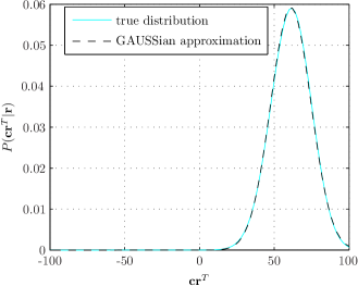
Figure 3: Distribution and its Gaussian Approximation

shows a distribution of the terminated $[7\;5]_{\mathrm{oct}}$ convolutional code as well the Gaussian approximation given the first two moments for a BSC.

V Conclusions

A trellis represents a general distribution which can be marginalized, e.g. with respect to edge labels. Two algorithms for computations on the trellis were presented: One allowing to calculate distributions, the other to compute their moments, allowing to approximate the distributions. The latter was derived by generalizing the forward/backward recursion as known from the BCJR algorithm. The results were transferred to the concrete problem of computing the moments of the conditional distribution of the correlation between a block code and some given word. The moment calculation algorithm is a requirement for efficient implementation of the discriminated belief propagation algorithm in [2]. It can also be used to calculate the conditional entropy of a code or sub-code. Though not the focus of this paper, in the Appendix it is shown that the algorithm does not restrict to calculation with real numbers, but is valid for any commutative semi-ring, thus providing a generalization of the Viterbi algorithm. The asymptotic complexity of the moment computation algorithm is the same as for the BCJR algorithm.

-A Relation between Uncertainty and Correlation

The conditional uncertainty of a code word $\mathbf{c}$ given a word $\mathbf{w}$ is defined as

$$H(\mathbf{c}|\mathbf{w}):=-\log_{2}P(\mathbf{c}|\mathbf{w})=-\log_{2}P(\mathbf{w}|\mathbf{c})+\underbrace{\log_{2}\frac{P(\mathbf{w})}{P(\mathbf{c})}}_{K_{1a}}$$

where $K_{1a}$ is a constant assuming equiprobable code words. Assuming further that $w_{i}$ is independent of $c_{j}$ for $i\neq j$ it follows that

$$\log_{2}P(\mathbf{w}|\mathbf{c}) = \log_{2}\prod_{i=1}^{n}P(w_{i}|c_{i})$$

$$= \sum_{i=1}^{n}\log_{2}P(w_{i}|c_{i})\;.$$

• For a binary symmetric channel (BSC) with $w_{i},c_{i}\in\{\pm 1\}$ and error probability $p$ the Hamming distance between $\mathbf{c}$ and $\mathbf{w}$ is $\frac{n-\mathbf{cw}^{T}}{2}$ which gives

  $$\log_{2}P(\mathbf{w}|\mathbf{c}) = \frac{n-\mathbf{cw}^{T}}{2}\log_{2}p+\frac{n+\mathbf{cw}^{T}}{2}\log_{2}(1-p)$$

  $$= \underbrace{\frac{n}{2}\log_{2}\left(p(1-p)\right)}_{K_{1b}}+\mathbf{cw}^{T}\cdot\underbrace{\frac{1}{2}\log_{2}\frac{1-p}{p}}_{K_{2}}.$$

• For an AWGN channel with noise variance $\sigma^{2}$ we obtain (note that $P(\mathbf{w}|\mathbf{c})$ actually is the Gauss probability density)

  $$\log_{2}P(\mathbf{w}|\mathbf{c}) = \sum_{i=1}^{n}\log_{2}\frac{1}{\sqrt{2\pi}\sigma}\exp\left(-\frac{(w_{i}-c_{i})^{2}}{2\sigma^{2}}\right)$$

  $$= \sum_{i=1}^{n}\left(\log_{2}\frac{1}{\sqrt{2\pi}\sigma}-\frac{(w_{i}-c_{i})^{2}}{2\sigma^{2}\cdot\ln 2}\right)$$

  $$= n\log_{2}\frac{1}{\sqrt{2\pi}\sigma}-\frac{1}{2\sigma^{2}\cdot\ln 2}\sum_{i=1}^{n}\left(c_{i}^{2}+w_{i}^{2}-2c_{i}w_{i}\right)$$

  $$= \underbrace{n\log_{2}\frac{1}{\sqrt{2\pi}\sigma}-\frac{n+\mathbf{w}\mathbf{w}^{T}}{2\sigma^{2}\cdot\ln 2}}_{K_{1b}}+\mathbf{cw}^{T}\cdot\underbrace{\frac{1}{\sigma^{2}\cdot\ln 2}}_{K_{2}}\,.$$

In either case we can thus express the conditional uncertainty as

$$H(\mathbf{c}|\mathbf{w})=\underbrace{\left(K_{1a}-K_{1b}\right)}_{K_{1}}-K_{2}\cdot\mathbf{cw}^{T}\>,$$

I.e., the uncertainty is linearly related to the correlation.

-B Calculating the Actual Distribution

For a trellis of rank $n$ and $g_{i}(e)\in\{\pm 1\}$, which is the case for hard decision decoding, the domain of the distributions, i.e., the values that $f(\mathtt{P})$ can take, is $\mathbb{D}=\{-n,-n+2,\dots,n-2,n\}$ with cardinality $\left|\mathbb{D}\right|=n+1$. In this case the distributions can be directly implemented as vectors of length $n+1$. A shift $\boxplus$ of the domain is simply a shift of the vector contents, and the correlation operation $*$ is discrete.

In case of soft decision, the domain needs to be quantized. For Gaussian distributions, an efficient way for uniform mid-tread quantization is to carry along the mean value $\mu$ of the distribution and to arrange the partitions equally to both sides of it, storing the partition contents in vectors $\mathbf{d}$. When extending a path $\mathtt{P}$ by an edge $e\in\mathbb{E}_{i-1,i}$ in the forward/backward recursion (lengthening), the domain of $f(\mathtt{P})$ is shifted by $g_{i}(e)$, i.e., $g_{i}(e)$ is added to the $\mu$. However, when joining paths in a vertex, the mean values of the incoming path distributions do usually not coincide. Hence a new mean value $\mu_{\mathrm{new}}$ has to be determined and the partition contents need to be distributed.

Let the vectors $\mathbf{d}$ be of length $(2N+1)$, each element corresponding to a partition of width $\Delta_{w}\,$. The partitions are indexed by $j\in\{-N,-N+1,\dots,N\}$, where $j=0$ denotes the center partition around the mean value. The a mean value $\mu_{\mathrm{new}}$ is the weighted sum of the mean values $\mu_{\mathrm{in}}$ of the involved distributions in vectors $\mathbf{d}_{\mathrm{in}}$. E.g., for the forward recursion,

$$\mu_{\mathrm{new}}=\alpha^{\mu}(v):=\sum_{e:\mathrm{fin}(e)=v}\underbrace{\left(\alpha^{\mu}\left(\mathrm{init}(e)\right)+g_{i}(e)\right)}_{\mu_{\mathrm{in}}}\\ \cdot\underbrace{\frac{\lambda(e)\cdot\eta(A,\mathrm{init}(e))}{\sum_{e^{\prime}:\mathrm{fin}(e^{\prime})=v}\lambda(e^{\prime})\cdot\eta(A,\mathrm{init}(e^{\prime}))}}_{\mathrm{relative\,weight\,of\,edge\,}e},$$

with $\alpha^{\mathcal{D}}(A)=0$, where $\mu_{\mathrm{in}}$ is the mean value of the distribution $\alpha^{\mathcal{D}}\left(\mathrm{init}(e)\right)$ after lengthening by $g_{i}(e)$, and $\alpha^{\mu}(v)$ is the mean of the forward distribution $\alpha^{\mathcal{D}}(v)$. The final distribution vector $\mathbf{d}_{\mathrm{new}}=\alpha^{\mathbf{d}}(v)$ is the weighted sum of the vectors $\mathbf{d}_{\mathrm{out}}$ which are calculated by distributing the content of the vectors $\mathbf{d}_{\mathrm{in}}=\alpha^{\mathbf{d}}\left(\mathrm{init}(e)\right)$ according to the new partition margins with $\Delta_{\mu}=\mu_{\mathrm{new}}-\mu_{\mathrm{in}}$ as follows (cf. Figure 4).

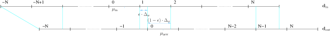
Figure 4: Assignment of Partition Contents of a Quantized Distribution

• $\epsilon=\frac{\Delta_{\mu}}{\Delta_{w}}-\left\lfloor\frac{\Delta_{\mu}}{\Delta_{w}}\right\rfloor\in[0,1)$

• $\mathbf{d}_{\mathrm{out}}=\mathbf{0}$ (all-zero vector)

• $\mathbf{d}_{\mathrm{out}}[-N]={\displaystyle\sum_{j=-N}^{-N+\left\lfloor\frac{\Delta_{\mu}}{\Delta_{w}}\right\rfloor}}\mathbf{d}_{\mathrm{in}}[j]$

• $\mathbf{d}_{\mathrm{out}}[N]=\sum_{j=N+\left\lfloor\frac{\Delta_{\mu}}{\Delta_{w}}\right\rfloor+1}^{N}\mathbf{d}_{\mathrm{in}}[j]$

• for $\max\left(-N,-N+\left\lfloor\frac{\Delta_{\mu}}{\Delta_{w}}\right\rfloor+1\right)\leq j\leq\min\left(N,N+\left\lfloor\frac{\Delta_{\mu}}{\Delta_{w}}\right\rfloor\right)$

  • $\mathbf{d}_{\mathrm{out}}[j-\left\lfloor\frac{\Delta_{\mu}}{\Delta_{w}}\right\rfloor-1]\hskip 2.84526pt+=\epsilon\cdot\mathbf{d}_{\mathrm{in}}[j]$

  • $\mathbf{d}_{\mathrm{out}}[j-\left\lfloor\frac{\Delta_{\mu}}{\Delta_{w}}\right\rfloor]\hskip 2.84526pt+=(1-\epsilon)\cdot\mathbf{d}_{\mathrm{in}}[j]$

where $a\hskip 2.84526pt+=b$ denotes the addition of $b$ to $a$, i.e., $a=a+b$. The forward distribution vector $\alpha^{\mathbf{d}}(A)$ is initialized The backward distribution is computed analogously.

With the two procedures of lengthening and joining the mean value of the symbol distribution can be calculated by

$$\Omega_{i}^{\mu}(x,T)=\sum_{{e\in E_{i-1,i}:\atop c(e)=x}}\underbrace{\left(\alpha^{\mu}\left(\mathrm{init}(e)\right)+g_{i}(e)+\beta^{\mu}\left(\mathrm{fin}(e)\right)\right)}_{\mu_{\mathrm{in}}}\\ \cdot\underbrace{\frac{\eta(A,\mathrm{init}(e))\cdot\lambda(e)\cdot\eta(\mathrm{fin}(e),B)}{\sum_{e^{\prime}\in E_{i-1,i}:c(e^{\prime})=x}\eta(A,\mathrm{init}(e^{\prime}))\cdot\lambda(e^{\prime})\cdot\eta(\mathrm{fin}(e^{\prime}),B)}}_{\mathrm{relative\,weight\,of\,edge\,}e},$$

and the discrete symbol distribution vector $\mathbf{d}_{\mathrm{out}}=\Omega_{i}^{\mathbf{d}}(x,T)$ is obtained by convolving the forward and backward distribution vectors $\alpha^{\mathbf{d}}\left(\mathrm{init}(e)\right)$ and $\beta^{\mathbf{d}}\left(\mathrm{fin}(e)\right)$ for each edge $e\in\mathbb{E}_{i-1,i}:c(e)=x$,

$$\mathbf{d}_{\mathrm{in}}=\alpha^{\mathbf{d}}\left(\mathrm{init}(e)\right)*\beta^{\mathbf{d}}\left(\mathrm{fin}(e)\right),$$

followed by a weighted re-distribution of the vector contents of the $\mathbf{d}_{\mathrm{in}}$ to $\mathbf{d}_{\mathrm{out}}$.

-C Generalization to Calculations on a Semi-ring

In the main part of this paper, the computation of moments in the trellis is introduced for real numbers. However, the algorithm is valid for the more general algebraic structure of commutative semi-rings. The $0$-th forward moment then results in the Viterbi algorithm on semi-rings.

Let the $\lambda$-label and the $c$-label come from an algebraic set $\mathbb{S}$ which is closed under the two binary operations $\oplus$ and $\odot$, called addition and multiplication, which satisfy the following axioms:

• The operation $\odot$ is associative and commutative, and there is an identity element $1^{\odot}$ such that $s\odot 1^{\odot}=1^{\odot}\odot s=s$ for all $s\in\mathbb{S}$, making $(\mathbb{S},\odot)$ a commutative monoid.

• The operation $\oplus$ is associative and commutative, and there is an identity element $0^{\oplus}$ such that $s\oplus 0^{\oplus}=0^{\oplus}\oplus s=s$ for all $s\in\mathbb{S}$, making $(\mathbb{S},\oplus)$ a commutative monoid.

• The distributive law $(x\oplus y)\odot z=(x\odot z)\oplus(y\odot z)$, for all triples $(x,y,z)$ from $\mathbb{S}$.

• The identity element $0^{\oplus}$ of the addition annihilates $\mathbb{S}$, i.e., $0^{\oplus}\odot s=s\odot 0^{\oplus}=0^{\oplus}$ for all $s\in\mathbb{S}$.

The triple $(\mathbb{S},\odot,\oplus)$ is called a commutative semiring.

Let $a,b\in(\mathbb{S},\odot,\oplus)$ be elements of such a commutative semiring. We define the following notation:

$$a^{m} := \begin{cases}\underbrace{a\odot a\odot\dots\odot a}_{m}&m\in\mathbb{N}\\ 1^{\odot}&m=0\end{cases}$$

$$na := \begin{cases}\underbrace{a\oplus a\oplus\dots\oplus a}_{n}={\displaystyle\mathop{\sum\oplus}_{i=1}^{n}}\,a&n\in\mathbb{N}\\ 0^{\oplus}&n=0\end{cases}$$

with $n\,a\odot b=n\,(a\odot b)$ and $\mathbb{N}$ being the set of natural numbers. Then the binomial theorem can be written as

$$(a\oplus b)^{m}=\mathop{\sum\oplus}_{l=0}^{m}{m\choose l}a^{l}\odot b^{m-l},\;m,l\in\mathbb{N}_{0},\;a,b\in(\mathbb{S},\odot,\oplus)$$

with the binomial coefficient ${m\choose l}\in\mathbb{N}_{0}=\left\{\mathbb{N}\cup 0\right\}$. In analogy to Definition 3 and Theorem 1 we can now define the forward numerator and its calculation on a semi-ring.

Definition 7

We define the $m$-th forward numerator of a function $f\in(\mathbb{S},\odot,\oplus)$ at vertex $v$ of a trellis $T$ as

$$\alpha^{(m)}(v):=\mathop{\sum\oplus}_{\mathtt{P}:A\rightarrow v}\lambda(\mathtt{P})\odot\left(f(\mathtt{P})\right)^{m}$$ (15)

with initial values

$$\alpha^{(m)}(A):=\left\{\begin{array}[]{ccc}1^{\odot}&:&m=0\\ 0^{\oplus}&:&m>0\end{array}\right..$$

Theorem 7

The $m$-th forward moment $\alpha^{(m)}(v)$ of a vertex $v\in V_{i}$ on depth $i$ can be recursively calculated on a trellis $T$ and a commutative semiring $(\mathbb{S},\odot,\oplus)$ by

$$\alpha^{(m)}(v)=\mathop{\sum\oplus}_{e:\mathrm{fin}(e)=v}\lambda(e)\odot\mathop{\sum\oplus}_{l=0}^{m}{m\choose l}\left(g_{i}(e)\right)^{l}\odot\alpha^{(m-l)}\left(\mathrm{init}(e)\right)$$ (16)

for all functions $f(\mathtt{P}:A\rightarrow v)$ and $g_{j}$, $j=1,\dots,i$, which fulfill

$$f(\mathtt{P})=f(e_{1}e_{2}\cdots e_{i})=g_{1}(e_{1})\oplus g_{2}(e_{2})\oplus\dots\oplus g_{i}(e_{i}).$$ (17)

Proof:

The proof is by induction on $\mathrm{depth}(v)$. For $\mathrm{depth}(v)=1$ the algorithm computes

$$\alpha^{(m)}(v) = \mathop{\sum\oplus}_{e:\mathrm{fin}(e)=v}\lambda(e)\odot\left(1\>\left(g_{1}(e)\right)^{m}\odot 1^{\odot}\right)$$

$$= \mathop{\sum\oplus}_{e:\mathrm{fin}(e)=v}\lambda(e)\odot\left(g_{1}(e)\right)^{m}$$

which is, as required, the sum of the labels on all edges $e$ joining $A$ to $v$, weighted by $\left(g_{1}(e)\right)^{m}$. For a vertex $v$ at depth $i+1$ the value assigned to $\alpha^{(m)}(v)$ is by the induction hypothesis

$$\alpha^{(m)}(v)=\mathop{\sum\oplus}_{e:\mathrm{fin}(e)=v}\lambda(e)\odot\mathop{\sum\oplus}_{l=0}^{m}{m\choose l}\left(g_{i}(e)\right)^{l}\\ \odot\mathop{\sum\oplus}_{\mathtt{P}:A\rightarrow\mathrm{init}e}\lambda(\mathtt{P})\odot\left(f(\mathtt{P})\right)^{m-l}.$$

Using the axioms of the commutative semiring $(\mathbb{S},\odot,\oplus)$ we have

$$\alpha^{(m)}(v)=\mathop{\sum\oplus}_{e:\mathrm{fin}(e)=v}\mathop{\sum\oplus}_{\mathtt{P}:A\rightarrow\mathrm{init}e}\lambda(e)\odot\lambda(\mathtt{P})\\ \odot\mathop{\sum\oplus}_{l=0}^{m}{m\choose l}\left(g_{i}(e)\right)^{l}\odot\left(f(\mathtt{P})\right)^{m-l}.$$

Applying Equation (17) and the binomial theorem we obtain

$$\alpha^{(m)}(v)=\mathop{\sum\oplus}_{e:\mathrm{fin}(e)=v}\mathop{\sum\oplus}_{\mathtt{P}:A\rightarrow\mathrm{init}e}\lambda(\mathtt{P}e)\odot\left(f(\mathtt{P})\oplus g_{i}(e)\right)^{m}.$$

But every path from $A$ to $v$ must be of the form $\mathtt{P}e$, where $\mathtt{P}$ is a path from $A$ to a vertex $u$ with $\mathrm{depth}(u)=i$, $\mathrm{init}(e)=u$ and $\mathrm{fin}(e)=v$. Hence, $\alpha^{(m)}(v)$ is correctly calculated by the theorem. ∎

Remark 11

Note that the complexity considerations in Theorems 2 and 5 transfer to the calculation on semi-rings. However, the terminology of “addition” and “multiplication” then refers to the operations $\oplus$ and $\odot$.

References

- [1] L. Bahl, J. Cocke, F. Jelinek, and J. Raviv. Optimal decoding of linear codes for minimizing symbol error rate. Information Theory, IEEE Transactions on, Volume 20:Page(s):284 – 287, March 1974.
- [2] U. Sorger. Discriminated Belief Propagation. Technical Report TR-CSC-07-01, Computer Science and Communications Research Unit, Université du Luxembourg, 2007. http://wiki.uni.lu/csc/Discriminator+Based+Decoding.html.
- [3] A.J. Viterbi. Error bounds for convolutional codes and an asymptotically optimum decoding algorithm. Information Theory, IEEE Transactions on, Volume 13:Page(s):260 – 269, April 1967.
- [4] G.D. Forney, Jr. Review of random tree codes. Appendix a, final report, contract nas2-3637, nasa cr73176, nasa ames res. ctr., moffett field, ca, Dec. 1967.
- [5] J.K. Wolf. Efficient maximum-likelihood decoding of linear block codes using a trellis. Information Theory, IEEE Transactions on, vol.24(no.1):pp. 76–80, Jan. 1978.
- [6] J.L. Massey. Foundation and methods of channel encoding. In in Proc. Int. Conf. Inform. Theory Syst., volume vol.65, Sept. 1978.
- [7] G.D. Forney, Jr. Coset codes. ii. binary lattices and related codes. Information Theory, IEEE Transactions on, Volume 34:Page(s):1152 – 1187, Sep 1988.
- [8] R.J. McEliece. On the BCJR Trellis for Linear Block Codes. IEEE Transactions on Information Theory, Vol. 42(No. 4):Pages: 1072 – 1092, July 1996.
- [9] S.M. Aji and R.J. McEliece. The generalized distributive law. Information Theory, IEEE Transactions on, Volume: 46:On page(s): 325–343, Mar 2000.
- [10] F.R. Kschischang, B.J. Frey, and H.-A. Loeliger. Factor graphs and the sum-product algorithm. Information Theory, IEEE Transactions on, Volume: 47:On page(s): 498–519, Feb 2001.