Assuming that the dilaton is the dark matter of the universe, we propose an experiment to detect the relic dilaton using the electromagnetic resonant cavity, based on the dilaton-photon conversion in strong electromagnetic background. We calculate the density of the relic dilaton, and estimate the dilaton mass for which the dilaton becomes the dark matter of the universe. With this we calculate the dilaton detection power in the resonant cavity, and compare it with the axion detection power in similar resonant cavity experiment.

Dilaton as a Dark Matter Candidate and Its Detection

I Introduction

One of the important issues in cosmology is the search for the dark matter. The notable candidates among many dark matter candidates are the dilaton and axion prd90 ; sik . The two particles differ completely in their origins, but are very similar in their coupling to the electromagnetic field and the fermionic matter fields. The dilaton is a universal scalar field which appears in all higher-dimensional unified theories (including the Kaluza-Klein theory and the superstring theory) which plays the role of the scalar graviton, and thus couples directly to all matter fields jmp75 ; duff ; witt . On the other hand, the axion is a pseudoscalar Goldstone boson generated by spontaneous breakdown of the Peccei-Quinn $U_{PQ}(1)$ symmetry which was introduced to solve the so called “strong CP problem” in strong interaction pec ; wein . But they have almost identical electromagnetic coupling, except that the dilation (being a scalar) couples to $F_{\mu\nu}^{2}$ while the axion (being a pseudoscalar) couples to $F_{\mu\nu}{\tilde{F}}_{\mu\nu}$. In this sense the dilaton and axion may be viewed as the scalar-pseudoscalar partners of each other. This is particularly true for the gravitational axion, the pseudoscalar graviton which has been proposed by Ni independent of the strong CP problem ni .

The axion has been believed to be one of the strong candidates of the dark matter by many physicists, and experiments to detect it have been actively performed sik ; asz . In comparison, the detection of the dilaton has not so actively been performed up to now, in spite of its theoretical importance. It is well known that the dilaton generates the fifth force which can affect the Einstein’s gravity in a fundamental way prd87 ; grg91 . Moreover, in cosmology it can play the role of the inflaton, and can be an excellent candidate of the dark matter prd90 ; cqg98 . In this paper we study the dilaton as a candidate of dark matter in detail, and propose a dilaton detection experiment using an electromagnetic resonant cavity. In particular, we refine the existing estimate of the dilaton mass, calculate the dilaton detection power in the resonant cavity, and compare this with the axion detection power in similar experiments.

The paper is organized as follows. In Section II we briefly review the dilaton physics based on Kaluza-Klein theory. In particular, we discuss how the dilaton mass can resolve the hierarchy problem and determine the size of the internal space. In Section III we discuss the role of dilaton in cosmology, and estimate the number density of the relic dilaton in the present universe based on the dilaton decay to two photons and fermion-antifermion pairs. In Section IV we discuss the condition for the dilaton to be a candidate of dark matter, and refine the acceptable mass range of dilaton. In Section V we propose the experiment to detect the dilaton using an electromagnetic resonant cavity. We calculate the dilaton detection power in the resonant cavity, and compare it with the axion detection power in similar experiments. Finally in Section VI we discuss the physical implications of our analysis.

II Dilatonic Fifth Force and Hierarchy Problem

All known interactions are mediated by spin-one or spin-two fields. However, the unification of all interactions inevitably requires the existence of a fundamental spin-zero field. In fact, all modern unified theories (Kaluza-Klein theory, supergravity, and superstring) contain a fundamental scalar field called the dilaton, or more precisely the Kaluza-Klein dilaton jmp75 ; prd87 . What makes this scalar field unique is that unlike others scalar fields like the Higgs field, it couples directly to the (trace of the) energy-momentum tensor of the matter fields. As such it plays the role of the scalar graviton, and generates the dilatonic fifth force which modifies Einstein’s gravity in a fundamental way.

Actually the simplest unified theory which contains the dilaton is the Brans-Dicke theory bra ; prl92 . Unfortunately the Brans-Dicke dilaton is proposed as a massless scalar graviton, so that it must create a long range fifth force which is comparable to Newton’s gravitational force. This contradicts the experiments which tell that such long range fifth force does not exist in nature exp1 ; exp2 . This rules out the Brans-Dicke theory as unphysical. On the other hand, the Kaluza-Klein dilaton has no such problem, because it naturally acquires a mass and generates a short range fifth force which does not contradict all known experiments jmp75 ; prd87 . So we will discuss the Kaluza-Klein dilaton in detail in the following.

The Kaluza-Klein dilaton plays a crucial role to resolve the so called hierarchy problem. It has been very difficult to understand why the Planck mass fixed by the Newton’s constant is so large compared to the mass scale of ordinary elementary particles, or equivalently why the gravitational force is so weak compared to other forces. There have been many proposals to resolve this problem. Long time ago Dirac conjectured that the Newton’s constant may not be a constant but actually a time-dependent parameter to resolve the problem dirac . Another proposal based on the higher-dimensional unification is that the gravitational force in higher-dimension is actually as strong as other forces, but a relatively large (compared to the Planck scale) internal space of the order of TeV scale makes the 4-dimensional gravitational force very weak ark ; dim . In this section we show that the dilaton plays the pivotal role in both proposals to resolve the hierarchy problem.

Since all higher-dimensional unified theories contain the $(4+n)$-dimensional gravitation, we start from the Kaluza-Klein theory. To obtain the $4$-dimensional effective theory one has to make the dimensional reduction. A simple and elegant way to do this is to impose an isometry jmp75 ; pen . In this dimensional reduction by isometry one may view the $(4+n)$-dimensional unified space as a principal fiber bundle P(M,G) made of the $4$-dimensional space-time manifold M as the base manifold and $n$-dimensional group manifold G as the vertical fiber (the internal space) on which G acts as an isometry group. Let $\gamma_{\mu\nu}$ and $\tilde{\phi}_{ab}$ be the 4-dimensional metric on M and the n-dimensional metric on G, $\gamma$ and $\tilde{\phi}$ be the determinants of $\gamma_{\mu\nu}$ and $\tilde{\phi}_{ab}$, and $\rho_{ab}=\tilde{\phi}_{ab}/\root n \of{\tilde{\phi}}$ ($|\textrm{det}\rho_{ab}|=1$) be the normalized metric on G. In this setting the (4+n)-dimensional Einstein-Hilbert action on P leads to the following 4-dimensional Lagrangian in the Jordan frame jmp75

$$\mathcal{L}_{CF}=-\displaystyle\frac{\hat{V}_{G}}{16\pi G_{P}}\sqrt{\vphantom{\tilde{\phi}}\gamma}\sqrt{\tilde{\phi}}~{}\Bigg{[}~{}~{}R_{M}-\displaystyle\frac{n-1}{4n}\gamma^{\mu\nu}\displaystyle\frac{(\partial_{\mu}\tilde{\phi})(\partial_{\nu}\tilde{\phi})}{\tilde{\phi}^{2}}+\displaystyle\frac{\kappa^{2}}{4}\root n \of{\tilde{\phi}}~{}\rho_{ab}\gamma^{\mu\alpha}\gamma^{\nu\beta}F_{\mu\nu}^{a}F_{\alpha\beta}^{b}$$

$$+\displaystyle\frac{\gamma^{\mu\nu}}{4}(D_{\mu}\rho^{ab})(D_{\nu}\rho_{ab})+\displaystyle\frac{1}{\kappa^{2}\root n \of{\tilde{\phi}}}~{}\hat{R}_{G}(\rho_{ab})+\Lambda_{P}+\lambda(|\textrm{det}\rho_{ab}|-1)~{}\Bigg{]},$$ (1)

where $G_{P}$ is the (4+n)-dimensional Newton’s constant, $\hat{V}_{G}$ is the normalized volume of the internal space G, $R_{M}$ is the scalar curvature of M fixed by $\gamma_{\mu\nu}$, $\hat{R}_{G}(\rho_{ab})$ is the normalized internal curvature fixed by $\rho_{ab}$, $\kappa$ is the unit scale of the internal space G, $F_{\mu\nu}^{a}$ is the gauge field of the isometry group G, $\Lambda_{P}$ is a (4+n)-dimensional cosmological constant, and $\lambda$ is a Lagrange multiplier.

Notice that the scalar field $\tilde{\phi}$ couples non-minimally to $R_{M}$, so that the metric $\gamma_{\mu\nu}$ does not describe the massless spin-two graviton prl92 . To cure this defect and discuss the physics of (1), we have to choose the physical conformal frame in which the metric describes the massless spin-two graviton. Let $<\tilde{\phi}>={v_{0}}^{2}$ and introduce the Pauli metric $g_{\mu\nu}$ and the Kaluza-Klein dilaton $\sigma$ by

$$g_{\mu\nu}=\exp\Big{(}\sqrt{\displaystyle\frac{n}{n+2}}~{}\sigma\Big{)}\gamma_{\mu\nu}~{},~{}~{}~{}~{}~{}~{}~{}\tilde{\phi}=\Big{[}v_{0}~{}\exp\Big{(}\sqrt{\displaystyle\frac{n}{n+2}}~{}\sigma\Big{)}\Big{]}^{2}.$$ (2)

The reason why we call $\sigma$ the dilaton is obvious. It determines the local dilatation in the conformal transformation. With this we find the following Lagrangian in the Pauli frame prd90 ; prd87 ,

$$\mathcal{L}_{CF}=-\displaystyle\frac{v_{0}\hat{V}_{G}}{16\pi G_{P}}\sqrt{g}\Big{[}R+\frac{1}{2}(\partial_{\mu}\sigma)^{2}-\displaystyle\frac{1}{4}(D_{\mu}\rho^{ab})(D^{\mu}{\rho}_{ab})$$

$$+\kappa^{-2}{v_{0}}^{-2/n}\hat{R}_{G}(\rho_{ab})\exp\Big{(}-\sqrt{\displaystyle\frac{n+2}{n}}~{}\sigma\Big{)}+\Lambda_{P}\exp\Big{(}-\sqrt{\displaystyle\frac{n}{n+2}}~{}\sigma\Big{)}$$

$$+\lambda\exp\Big{(}-\sqrt{\displaystyle\frac{n}{n+2}}\sigma\Big{)}(|\textrm{det}\rho_{ab}|-1)+\displaystyle\frac{\kappa^{2}}{4}{v_{0}}^{2/n}\exp\Big{(}\sqrt{\displaystyle\frac{n+2}{n}}~{}\sigma\Big{)}\rho_{ab}F_{\mu\nu}^{a}F^{\mu\nu b}~{}\Big{]}$$

$$=-\displaystyle\frac{\sqrt{g}}{16\pi G}\Big{[}R+\frac{1}{2}(\partial_{\mu}\sigma)^{2}-\displaystyle\frac{1}{4}(D_{\mu}\rho^{ab})(D^{\mu}{\rho}_{ab})$$

$$+\displaystyle\frac{1}{16\pi G}{v_{0}}^{-2/n}\hat{R}_{G}(\rho_{ab})\exp\Big{(}-\sqrt{\displaystyle\frac{n+2}{n}}~{}\sigma\Big{)}+\Lambda_{P}\exp\Big{(}-\sqrt{\displaystyle\frac{n}{n+2}}~{}\sigma\Big{)}$$

$$+\lambda\exp\Big{(}-\sqrt{\displaystyle\frac{n}{n+2}}\sigma\Big{)}(|\textrm{det}\rho_{ab}|-1)+4\pi G\exp\Big{(}\sqrt{\displaystyle\frac{n+2}{n}}~{}\sigma\Big{)}\rho_{ab}{\hat{F}}_{\mu\nu}^{a}{\hat{F}}^{\mu\nu b}~{}\Big{]},$$ (3)

where we have put

$$\displaystyle\frac{v_{0}\hat{V}_{G}}{16\pi G_{P}}=\displaystyle\frac{1}{16\pi G},~{}~{}~{}~{}~{}\displaystyle\frac{\kappa^{2}}{16\pi G}=1,$$ (4)

and renormalized the field strength $F_{\mu\nu}^{a}$ to ${\hat{F}}_{\mu\nu}^{a}={v_{0}}^{1/n}F_{\mu\nu}^{a}$ to assure the minimal coupling of the Pauli metric to the gauge field.

Notice that the unit scale of the internal space $\kappa$ is fixed by the Planck scale $\sqrt{16\pi G}$, but the actual scale of the internal space is given by ${v_{0}}^{1/n}\kappa$, because the vacuum expectation value of the volume of the internal space is fixed by

$$<V_{G}>=\sqrt{<\tilde{\phi}>}~{}\hat{V}_{G}=v_{0}~{}\hat{V}_{G}\simeq v_{0}~{}\kappa^{n}\simeq v_{0}~{}(16\pi G)^{n/2}.$$ (5)

This tells that the scale of the higher-dimensional gravitational constant $G_{P}$ need not be fixed by the Planck scale, because it is given by prd90 ; grg91

$${G_{P}}^{1/(n+2)}=(16\pi)^{n/2(n+2)}~{}{v_{0}}^{1/(n+2)}~{}G^{1/2}.$$ (6)

So, with a large $v_{0}$, one can easily bring the length scale $\root(n+2) \of{G_{P}}$ to the order of the elementary particle length scale. Indeed, $n=2$ brings the Plank scale down to TeV scale when the scale of the internal space becomes of the order of $10^{-1}\rm{cm}$. This is precisely the proposal which has been popularized to resolve the hierarchy problem ark ; dim .

Now we show how the dilaton can resolve the hierarchy problem. Consider the gravitational coupling to the gauge field in (3). Here the dilaton modifies $G$ to $G\exp[\sqrt{(n+2)/n}~{}\sigma]$, which can be interpreted as a space-time dependent Newton’s constant. So the dilaton transforms the hierarchy problem to a space-time dependent artifact jmp75 ; prd87 . And this is precisely the Dirac’s proposal to resolve the hierarchy problem. Furthermore, with a large internal space, we can show that the dilaton can bring down the Planck mass to the ordinary elementary particle mass. To see this, suppose the Lagrangian (3) has the unique vacuum at

$$<g_{\mu\nu}>=\eta_{\mu\nu},~{}~{}~{}<\sigma>=0,~{}~{}~{}<\rho_{ab}>=\delta_{ab},~{}~{}~{}<A_{\mu}^{a}>=0.$$ (7)

Then we have the following dilatonic potential $V(\sigma)$ prd87 ; prd90

$$V(\sigma)=\displaystyle\frac{1}{16\pi G}\Big{[}\displaystyle\frac{\hat{R}_{G}}{16\pi G}~{}{v_{0}}^{-2/n}~{}\exp(-\sqrt{\displaystyle\frac{n+2}{n}}~{}\sigma)+\Lambda_{P}~{}\exp(-\sqrt{\displaystyle\frac{n}{n+2}}~{}\sigma)\Big{]}+V_{0}$$

$$=\displaystyle\frac{\hat{R}_{G}}{(16\pi G)^{2}}~{}{v_{0}}^{-2/n}~{}\Big{[}\exp(-\sqrt{\displaystyle\frac{n+2}{n}}~{}\sigma\big{)}-\displaystyle\frac{n+2}{n}~{}\exp(-\sqrt{\displaystyle\frac{n}{n+2}}~{}\sigma)+\displaystyle\frac{2}{n}\Big{]},$$ (8)

where $\hat{R}_{G}=\hat{R}_{G}(<\delta_{ab}>)$ is the dimensionless vacuum curvature of the internal space $G$ obtained by the bi-invariant Cartan-Killing metric $\delta_{ab}$

$$\hat{R}_{G}=-\displaystyle\frac{1}{2}f_{ab}^{~{}~{}d}f_{cd}^{~{}~{}b}\delta^{ac}-\displaystyle\frac{1}{4}f_{ab}^{~{}~{}m}f_{cd}^{~{}~{}n}\delta^{ac}\delta^{bd}\delta_{mn},$$ (9)

and $V_{0}$ is a constant which assures that (8) does not create non-vanishing 4-dimensional cosmological constant (vacuum energy). An important point here is that $\Lambda_{P}$ and $V_{0}$ are completely fixed by the vacuum condition $dV(0)/d\sigma=0$ and $V(0)=0$,

$$\Lambda_{P}=-\displaystyle\frac{n+2}{n}~{}{v_{0}}^{-2/n}~{}\displaystyle\frac{\hat{R}_{G}}{16\pi G},~{}~{}~{}~{}~{}V_{0}=\displaystyle\frac{2}{n}~{}{v_{0}}^{-2/n}~{}\displaystyle\frac{\hat{R}_{G}}{(16\pi G)^{2}}.$$ (10)

With this we find the following mass $\mu$ of the Kaluza-Klein dilaton,

$$\mu^{2}=(16\pi G)~{}\displaystyle\frac{d^{2}V(0)}{d\sigma^{2}}=-{v_{0}}^{-2/n}~{}\displaystyle\frac{\hat{R}_{G}}{8\pi n~{}G}=-{v_{0}}^{-2/n}~{}\displaystyle\frac{\hat{R}_{G}}{8\pi n}~{}m_{p}^{2},$$ (11)

where $m_{p}\simeq 1.2\times 10^{19}~{}\mathrm{GeV}$ is the Planck mass. This confirms that when the internal space is of the Planck scale (i.e., when $v_{0}\simeq 1$) the dilaton mass becomes of the Planck mass. But remarkably, a large $v_{0}$ naturally reduces the dilaton mass to the order of the elementary particle mass scale when $\hat{R}_{G}\neq 0$ prd90 ; grg91 . In fact (11) tells that the dilaton mass is determined by the scale of the internal space $L_{G}$ as follows,

$$L_{G}={v_{0}}^{1/n}~{}\kappa=\sqrt{-\displaystyle\frac{2\hat{R}_{G}}{n}}~{}\displaystyle\frac{1}{\mu}\simeq\displaystyle\frac{1}{\mu}.$$ (12)

In particular, for the $S^{3}$ compactification of the $3$-dimensional internal space in $(4+3)$-dimensional unification with G=$SU(2)$, we have $\hat{R}_{G}=-3/2$ and $L_{G}=1/\mu$. This is how the dilaton resolves the hierarchy problem in Kaluza-Klein unification.

At this point it is important to compare (6) and (11). Both provide a resolution of the hierarchy problem, but there are important differences. First, (6) does that with the gravitational coupling strength, while (11) does that with the dilaton mass. Secondly, the dimension of the internal space $n$ plays the crucial role in (6), but the curvature of the internal space plays the crucial role in (11). In fact we have $\mu=0$ when $\hat{R}_{G}=0$, independent of $n$ and $v_{0}$. More importantly, (11) tells that a mass can be generated geometrically through the scalar curvature of the internal space prd87 ; prd90 . This demonstrates that there is another mass generation mechanism other than the Higgs mechanism, a geometric mass generation through the curvature of space-time. Understanding the origin of mass has been a fundamental problem in physics. Our analysis shows that the hierarchy problem is closely related to the problem of the origin of mass, and that the geometric mass generation provides a natural resolution to the problem of the origin of mass.

In superstring or supergravity unification the situation is similar but more complicated, because in this case one has other higher-dimensional matter fields prd87 ; cqg98 . For example, in superstring one has an extra higher-dimensional dilaton (the string dilaton) which remains massless in all orders of perturbation, so that one has to find out a natural mechanism to make the dilaton massive first witt . Other than these complications the generic features of the dilaton physics remain the same. This makes the dilaton a fundamental scalar field of nature which one can not ignore.

The dilaton has been called in various names, recently by the radion ark or the chameleon kho . But we notice that the dilaton as the scalar graviton has a long history. The first such dilaton was the Brans-Dicke dilaton introduced by Jordan and independently by Brans and Dicke bra . Subsequently the Kaluza-Klein dilaton jmp75 and string dilaton witt have been introduced. Later, the dilaton has been re-invented by many authors in so-called “the scalar field models”. Among these only the Kaluza-Klein dilaton naturally acquires the mass and thus can describe a realistic scalar graviton.

As we have remarked an immediate consequence of the dilaton is the presence of dilatonic fifth force which modifies Einstein’s gravitation prl92 . To see how the dilaton affect the gravitation we have to know the mass of dilation and its coupling strength to matter fields. In Kaluza-Klein theory the dilaton naturally acquires a mass as we have shown in (11). As for the dilatonic coupling to matter fields, the coupling may depend on the types of matter field it couples to prd87 ; prl92 . But in practice only one type of coupling, the dilatonic coupling to the baryonic matter, is important because this is what we measure in experiments. So, only two parameters, the baryonic coupling constant and the mass of the dilaton, becomes important to describe the dilatonic fifth-force. Let $F_{g}$ and $F_{5}$ be the gravitational and the fifth force between the two baryonic point particles separated by a distance $r$. From the dimensional argument, one may express the total force in the Newtonian limit as

$$F=F_{g}+F_{5}\simeq\frac{\alpha_{g}}{r^{2}}+\displaystyle\frac{\alpha_{5}}{r^{2}}~{}e^{-\mu r}=\displaystyle\frac{\alpha_{g}}{r^{2}}\big{(}1+\beta~{}e^{-\mu r}\big{)}$$ (13)

where $\alpha_{g}$, $\alpha_{5}$ are the fine structure constants of the gravitation and fifth force, and $\beta$ is the ratio between them. In terms of Feynman diagrams the first term represents one graviton exchange but the second term represents one dilaton exchange in the zero momentum transfer limit. In the Kaluza-Klein unification we have $\beta=n/(n+2)$ prd87 ; prd90 , but in general one may assume $\beta\simeq 1$ because the dilaton is the scalar partner of the graviton. With this assumption one may try to measure the range of the fifth force experimentally.

A recent torsion-balance fifth force experiment puts the upper bound of the range of the fifth force to be around $56~{}\mathrm{\mu m}$ with 95% confidence level exp1 ; exp2 . This tells that the dilaton mass has to be larger than $10^{-2}~{}\mathrm{eV}$. This, with (12), implies that, in the $(4+3)$-dimensional unification with the $S^{3}$ compactification of the internal space, the scale of the internal space $L_{G}$ is smaller than $44~{}\mathrm{\mu m}$. In the following, however, we will simply treat the dilaton mass an undetermined parameter, and find an independent estimate of the dilaton mass based on the assumption that the dilaton is the dark matter of the universe.

III Relic Dilaton in Cosmology

The dilaton has another important impact in cosmology. First of all, it could be a natural candidate for the dark matter of the universe prd90 ; cqg98 . The dilaton starts with the thermal equilibrium at the beginning and decouples from other sources very early near the Planck time. Moreover, since its coupling to matter fields is very weak, it may easily survive in the present universe and become the dark matter of the universe. In this section we estimate the density of the relic dilaton.

Let’s consider the dilaton in the early universe. From the dimensional argument one may assume the dilatonic coupling strength to matter fields to be $g~{}m/m_{p}$, where $g$ is the dimensionless coupling constant and $m$ is the mass of the relevant matter (e.g., quarks and gluons). But at high temperature (at $T\gg m$), the coupling strength can be written as $g~{}T/m_{p}$. With this one can easily estimate the dilaton creation (and annihilation) cross section as cqg98

$$\sigma\simeq g^{2}~{}\Bigg{(}\frac{T}{m_{p}}\Bigg{)}^{2}\times\frac{1}{T^{2}},$$ (14)

with the transition rates $\Gamma$

$$\Gamma\simeq N\sigma v\simeq g^{2}~{}\Bigg{(}\frac{T}{m_{p}}\Bigg{)}^{2}\times T,$$ (15)

where $N$ and $v$ are the density of the matter and the speed of the dilaton. Similarly the dilaton scattering cross section and the interaction rate are given by

$$\sigma\simeq g^{4}~{}\Bigg{(}\frac{T}{m_{p}}\Bigg{)}^{4}\times\frac{1}{T^{2}},~{}~{}~{}~{}~{}~{}\Gamma\simeq N\sigma v\simeq g^{4}~{}\Bigg{(}\frac{T}{m_{p}}\Bigg{)}^{4}\times T.$$ (16)

On the other hand, the Hubble expansion rate in the early universe is given by $H\simeq T^{2}/m_{p}$. So, letting $\Gamma\simeq H$ we find the dilaton decoupling temperature

$$T_{D}\simeq\displaystyle\frac{m_{p}}{g^{4/3}}.$$ (17)

This confirms that the dilaton is thermally produced at the beginning, and decouples from the other matters around the Planck time.

The dilaton becomes unstable and decays into ordinary matter. A typical decay process is the two-photon process and the fermion-antifermion pair production process. The Lagrangian (3) implies that, in the linear approximation where $\sigma$ is assumed small enough, the decay may be described by the following interaction Lagrangian,

$$\mathcal{L}_{int}\simeq-\frac{1}{4}g_{1}\sqrt{16\pi G}~{}\hat{\sigma}~{}F_{\mu\nu}F^{\mu\nu}-g_{2}\sqrt{16\pi G}~{}m~{}\hat{\sigma}~{}\bar{\psi}\psi,$$ (18)

where $g_{1}$ and $g_{2}$ are dimensionless coupling constants, $m$ is the mass of the fermion, and $\hat{\sigma}=\sigma/\sqrt{16\pi G}$ is the dimensional (physical) dilaton field. This should be compared to the following axion interaction Lagrangian given by sik ; ni ,

$$\mathcal{L}_{int}\simeq-\alpha_{\gamma}~{}a~{}F_{\mu\nu}\tilde{F}^{\mu\nu}-i\alpha_{f}~{}a~{}\bar{\psi}\gamma^{5}\psi,$$ (19)

where $a$ is the axion field, $\alpha_{\gamma}$ and $\alpha_{f}$ are the axion coupling constants. This confirms that dilaton and axion are the scalar-pseudoscalar counterparts of each other. Actually we can also include the following dilaton-fermion interaction in (18)

$$g_{3}\sqrt{16\pi G}~{}\hat{\sigma}~{}\bar{\psi}\gamma^{\mu}\partial_{\mu}\psi+g_{4}\sqrt{16\pi G}~{}\partial_{\mu}\hat{\sigma}~{}\bar{\psi}\gamma^{\mu}\psi.$$ (20)

But for simplicity we will concentrate on (18) in the following.

Consider the interaction between dilaton and photon first, and let’s introduce a dimensional coupling constant $\alpha_{1}=g_{1}\sqrt{16\pi G}/4$ and denote the dilaton mass by $\mu$. The differential dilaton decay rate to two photons at tree level is given by

$$d\Gamma_{\sigma\rightarrow\gamma\gamma}=\displaystyle\frac{1}{2p^{0}}\sum_{\lambda,\lambda^{\prime}=\pm 1}\displaystyle\frac{1}{2!}(2\pi)^{4}\delta^{(4)}(p^{\mu}-k^{\mu}-k^{\prime\mu})|M|^{2}\displaystyle\frac{d^{3}\vec{k}}{(2\pi)^{3}2k^{0}}\displaystyle\frac{d^{3}\vec{k^{\prime}}}{(2\pi)^{3}2k^{\prime 0}}~{},$$ (21)

$$M=-i\alpha_{1}\Big{(}k_{\mu}\epsilon_{\nu}(k,\lambda)-k_{\nu}\epsilon_{\mu}(k,\lambda)\Big{)}\Big{(}k^{\prime\mu}\epsilon^{\prime\nu}(k^{\prime},\lambda^{\prime})-k^{\prime\nu}\epsilon^{\prime\mu}(k^{\prime},\lambda^{\prime})\Big{)},$$ (22)

where $p^{\mu}$ and $k^{\mu},~{}k^{\prime\mu}$ are the 4-momenta of the incoming dilaton and the outgoing photons, $M$ is the reduced Feynman matrix element, $\epsilon^{\mu}(k,\lambda)$ and $\epsilon^{\prime\mu}(k^{\prime},\lambda^{\prime})$ are the transverse polarization vectors of photons. It is simple to calculate the matrix element in the center of momentum (COM) frame where $\vec{k^{\prime}}=-\vec{k}$. From

$$\Big{(}k_{\mu}\epsilon_{\nu}(k,\lambda)-k_{\nu}\epsilon_{\mu}(k,\lambda)\Big{)}\Big{(}k^{\prime\mu}\epsilon^{\prime\nu}(k^{\prime},\lambda^{\prime})-k^{\prime\nu}\epsilon^{\prime\mu}(k^{\prime},\lambda^{\prime})\Big{)}=2\Big{(}k_{\mu}k^{\prime\mu}\Big{)}\Big{(}\epsilon_{\nu}(k,\lambda)\epsilon^{\prime\nu}(k^{\prime},\lambda^{\prime})\Big{)},$$

$$k_{\mu}k^{\prime\mu}=-2|\vec{k}|^{2},~{}~{}~{}~{}~{}\displaystyle\frac{}{}\sum_{\lambda,\lambda^{\prime}}\Big{|}\epsilon_{\nu}(k,\lambda)\epsilon^{\prime\nu}(k^{\prime},\lambda^{\prime})\Big{|}^{2}=2,$$ (23)

we get the following decay rate,

$$\Gamma_{\sigma\rightarrow\gamma\gamma}=\displaystyle\frac{\alpha_{1}^{2}}{2\pi^{2}\mu}\int d^{3}\vec{k}~{}d^{3}\vec{k^{\prime}}|\vec{k}|^{2}\delta^{(4)}(k^{\mu}+k^{\prime\mu}-p^{\mu})$$

$$=\displaystyle\frac{\alpha_{1}^{2}}{2\pi^{2}\mu}\int d^{3}d^{3}\vec{k^{\prime}}\vec{k}~{}|\vec{k}|^{2}\delta(k^{0}+k^{\prime 0}-\mu)\delta^{(3)}(\vec{k}+\vec{k^{\prime}})=\displaystyle\frac{\alpha_{1}^{2}}{2\pi^{2}\mu}\int d^{3}\vec{k}~{}|\vec{k}|^{2}\delta(2k^{0}-\mu)$$

$$=\displaystyle\frac{\alpha_{1}^{2}}{2\pi^{2}\mu}\int d|\vec{k}|d\Omega_{\vec{k}}|\vec{k}|^{4}\frac{1}{2}\delta(|\vec{k}|-\mu/2)=\displaystyle\frac{\alpha_{1}^{2}\mu^{3}}{16\pi}.$$ (24)

With this we get the following life-time of the dilaton

$$\tau_{\sigma\rightarrow\gamma\gamma}=\displaystyle\frac{1}{\Gamma_{\sigma\rightarrow\gamma\gamma}}=\displaystyle\frac{16m_{p}^{2}}{g_{1}^{2}\mu^{3}}.$$ (25)

Notice that when $\mu\simeq m_{p}$, the dilaton has a very short life-time.

Now consider the dilaton-fermion interaction, and let $\alpha_{2}=g_{2}\sqrt{16\pi G}~{}m$ be the dimensionless coupling constant. The differential decay rate of dilaton to fermion and anti-fermion pair at tree level is written as

$$d\Gamma_{\sigma\rightarrow\bar{\psi}\psi}=\displaystyle\frac{1}{2p^{0}}\sum_{s,s^{\prime}=\pm\frac{1}{2}}(2\pi)^{4}\delta^{(4)}(p^{\mu}-k^{\mu}-k^{\prime\mu})|M|^{2}\displaystyle\frac{d^{3}\vec{k}}{(2\pi)^{3}2k^{0}}\displaystyle\frac{d^{3}\vec{k^{\prime}}}{(2\pi)^{3}2k^{\prime 0}},$$

$$M=-i\alpha_{2}\bar{u}(k,s)\textit{v}(k^{\prime},s^{\prime}),$$ (26)

where $p^{\mu}$ and $k^{\mu}$, $k^{\prime\mu}$ are the 4-momenta of the incoming dilaton and the outgoing fermion-antifermion pair, and $s,~{}s^{\prime}$ are the fermion spin indices. Using the well-known sum-rule gre ,

$$\sum_{s,s^{\prime}=\pm\frac{1}{2}}|\bar{u}(k,s)\textit{v}(k^{\prime},s^{\prime})|^{2}=4(-k_{\mu}k^{\prime\mu}-m^{2}),$$ (27)

we have the following decay rate,

$$\Gamma_{\sigma\rightarrow\bar{\psi}\psi}=\displaystyle\frac{\alpha_{2}^{2}}{8\pi^{2}p^{0}}\int\displaystyle\frac{d^{3}\vec{k}}{k^{0}}~{}\displaystyle\frac{d^{3}\vec{k^{\prime}}}{k^{\prime 0}}(-k_{\mu}k^{\prime\mu}-m^{2})\delta^{(4)}(k^{\mu}+k^{\prime\mu}-p^{\mu})$$

$$=\displaystyle\frac{\alpha_{2}^{2}}{8\pi^{2}p^{0}}\times\displaystyle\frac{\mu^{2}-4m^{2}}{2}\int\displaystyle\frac{d^{3}\vec{k}}{k^{0}}~{}\displaystyle\frac{d^{3}\vec{k^{\prime}}}{k^{\prime 0}}\delta^{(3)}(\vec{k}+\vec{k^{\prime}}-\vec{p})\delta(k^{0}+k^{\prime 0}-p^{0})$$

$$=\displaystyle\frac{\alpha_{2}^{2}}{8\pi^{2}\mu}\times\displaystyle\frac{\mu^{2}-4m^{2}}{2}\int\displaystyle\frac{d^{3}\vec{k}}{(k^{0})^{2}}\delta(2k^{0}-\mu)~{}~{}(\textrm{COM frame})$$

$$=\displaystyle\frac{\alpha_{2}^{2}}{8\pi^{2}\mu}\times\displaystyle\frac{\mu^{2}-4m^{2}}{2}\int d|\vec{k}|d\Omega_{\vec{k}}\displaystyle\frac{|\vec{k}|^{2}}{(k^{0})^{2}}\delta(2\sqrt{m^{2}+|\vec{k}|^{2}}-\mu)$$

$$=\displaystyle\frac{\alpha_{2}^{2}}{2\pi\mu}\times\displaystyle\frac{\mu^{2}-4m^{2}}{2}\times\displaystyle\frac{|\vec{k}|}{2(k^{0})}\Bigg{|}_{k^{0}=\mu/2}=\displaystyle\frac{\alpha_{2}^{2}\mu}{8\pi}\times\Bigg{[}1-\bigg{(}\displaystyle\frac{2m}{\mu}\bigg{)}^{2}\Bigg{]}^{3/2}.$$ (28)

So we have the following life-time of the dilaton

$$\tau_{\sigma\rightarrow\bar{\psi}\psi}=\frac{1}{\Gamma_{\sigma\rightarrow\bar{\psi}\psi}}=\frac{m_{p}^{2}}{2g_{2}^{2}m^{2}\mu}\Bigg{[}1-\bigg{(}\frac{2m}{\mu}\bigg{)}^{2}\Bigg{]}^{-3/2}.$$ (29)

Notice that this becomes comparable to (25) only when $m\sim 0.32\times\mu$, so that the two photon decay becomes the dominant decay of dilaton in general.

The dilaton number density $n$ after the decoupling is given by the well-known equation kol .

$$\displaystyle\frac{d(nR^{3})}{dt}=-\displaystyle\frac{1}{\tau}(nR^{3}),~{}~{}~{}~{}~{}\displaystyle\frac{dn}{dt}+3H~{}n=-\displaystyle\frac{1}{\tau}~{}n.$$ (30)

where $\tau$ is the total life-time, $R$ is the scale factor of the Friedmann-Robertson-Walker metric, and $H$ is the Hubble parameter. From this we have the familiar expression

$$n(t)=n_{D}\Bigg{(}\displaystyle\frac{R_{D}}{R}\Bigg{)}^{3}\textrm{exp}(-t/\tau),$$ (31)

where the subscript $D$ denotes the decoupling time. Note that the factor $1/R^{3}$ represents the dilution of the dilaton due to Hubble expansion. To find the present dilaton number density notice that in the highly relativistic regime (i.e., when $T\gg\mu$), the particle number density is given by kol ,

$$n_{b}=\displaystyle\frac{\zeta(3)}{\pi^{2}}gT^{3}~{}~{}~{}\textrm{(for a boson)},$$

$$n_{f}=\displaystyle\frac{3}{4}\displaystyle\frac{\zeta(3)}{\pi^{2}}gT^{3}~{}~{}~{}\textrm{(for a fermion)},$$ (32)

where $g$ is the internal degrees of freedom of the relevant particle and $\zeta(x)$ is the Riemann’s zeta function. So, at the time of dilaton decoupling, the dilaton number density $n_{D}$ is given by

$$n_{D} = \displaystyle\frac{\zeta(3)}{\pi^{2}}~{}T_{D}^{3}\simeq\displaystyle\frac{1.202}{\pi^{2}}~{}T_{D}^{3}.$$ (33)

On the other hand, the total entropy density $s$ of the universe is given by kol ,

$$s=\displaystyle\frac{2\pi^{2}}{45}g_{*}T^{3},$$

$$g_{*}=\displaystyle\frac{}{}\sum_{i=bosons}g_{i}\Bigg{(}\displaystyle\frac{T_{i}}{T}\Bigg{)}^{3}+\frac{7}{8}\sum_{i=fermions}g_{i}\Bigg{(}\displaystyle\frac{T_{i}}{T}\Bigg{)}^{3},$$ (34)

where $g_{i}$ and $T_{i}$ are the internal degrees of freedom and the thermal equilibrium temperature of the $i$-th particle, and $T$ is the thermal temperature of photon. At present we have $g_{*0}\simeq 3.91$ (with photon and three types of light neutrinos), but at the Plank time we have $g_{*}\simeq 106.75$ according to the standard model kol . Now, the total entropy conservation of the universe in the co-moving volume tells that ${g_{*}}_{D}T_{D}^{3}R_{D}^{3}={g_{*}}_{0}T_{0}^{3}R_{0}^{3}$. From this we get (with $T_{0}\simeq 2.73~{}\textrm{K}$) the present dilaton number density $n(t_{0})$,

$$n(t_{0})=n_{D}\Bigg{(}\displaystyle\frac{R_{D}}{R_{0}}\Bigg{)}^{3}\textrm{exp}(-t_{0}/\tau)=\displaystyle\frac{\zeta(3)}{\pi^{2}}~{}T_{D}^{3}\Bigg{(}\displaystyle\frac{R_{D}}{R_{0}}\Bigg{)}^{3}\textrm{exp}(-t_{0}/\tau)$$

$$=\displaystyle\frac{\zeta(3)}{\pi^{2}}\displaystyle\frac{{g_{*}}_{0}}{{g_{*}}_{D}}~{}T_{0}^{3}\text{exp}(-t_{0}/\tau)\simeq 7.5~{}\textrm{exp}(-t_{0}/\tau)~{}\textrm{cm}^{-3}.$$ (35)

Note that the coefficient $7.5~{}\mathrm{cm^{-3}}$ would be the present dilaton number density if the dilaton had not been decaying at all, which is half the present number density of the massless graviton.

IV Dilaton as a dark matter candidate

The above analysis implies that the dilaton with a proper mass can easily survive to present time, and could become the dark matter of the universe. Assuming this is the case, we can estimate the mass of the dilaton. It has been argued that there are two mass ranges of the relic dilaton, $\mu_{1}\simeq\textrm{500~{}eV}$ and $\mu_{2}\simeq\textrm{270~{}MeV}$, in which the relic dilaton could be the dominant matter of the universe cqg98 . This is because the dilaton with mass larger than $\mu_{2}$ does not survive long enough to become the dominant matter of the universe, and the dilaton with mass smaller than $\mu_{1}$ survives but fails to be dominant due to its low mass. The dilaton with mass in between cannot be seriously considered because it would overclose the universe. In this section we refine the above result.

$g_{1}\simeq g_{2}$	$\mu_{1}$	$\tau_{1}$	$\mu_{2}$	$\tau_{2}$
10	160 eV	$3.84\times 10^{33}$ sec	$75.6$ MeV	$3.62\times 10^{16}$ sec
5	160 eV	$1.53\times 10^{34}$ sec	$121$ MeV	$3.49\times 10^{16}$ sec
2	160 eV	$9.59\times 10^{34}$ sec	$219$ MeV	$3.35\times 10^{16}$ sec
1	160 eV	$3.84\times 10^{35}$ sec	$276$ MeV	$3.29\times 10^{16}$ sec
0.9	160 eV	$4.74\times 10^{35}$ sec	$292$ MeV	$3.27\times 10^{16}$ sec
0.8	160 eV	$6.00\times 10^{35}$ sec	$312$ MeV	$3.26\times 10^{16}$ sec
0.7	160 eV	$7.83\times 10^{35}$ sec	$341$ MeV	$3.25\times 10^{16}$ sec
0.6	160 eV	$1.07\times 10^{36}$ sec	$383$ MeV	$3.21\times 10^{16}$ sec
0.5	160 eV	$1.53\times 10^{36}$ sec	$445$ MeV	$3.19\times 10^{16}$ sec
0.4	160 eV	$2.40\times 10^{36}$ sec	$543$ MeV	$3.14\times 10^{16}$ sec
0.3	160 eV	$4.26\times 10^{36}$ sec	$702$ MeV	$3.09\times 10^{16}$ sec
0.2	160 eV	$9.60\times 10^{36}$ sec	$988$ MeV	$3.03\times 10^{16}$ sec
0.1	160 eV	$3.84\times 10^{37}$ sec	$1.68$ GeV	$2.94\times 10^{16}$ sec
0.05	160 eV	$1.53\times 10^{38}$ sec	$2.76$ GeV	$2.85\times 10^{16}$ sec
$10^{-2}$	160 eV	$3.84\times 10^{39}$ sec	$8.37$ GeV	$2.66\times 10^{16}$ sec
$10^{-3}$	160 eV	$3.84\times 10^{41}$ sec	$40.0$ GeV	$2.45\times 10^{16}$ sec
$10^{-4}$	160 eV	$3.84\times 10^{43}$ sec	$191$ GeV	$2.25\times 10^{16}$ sec

Table 1: The coupling constants versus dilaton mass and life-time, where we have assumed $g_{1}\simeq g_{2}$ . Here the smaller mass is denoted by $\mu_{1}$ and larger mass is denoted by $\mu_{2}$, and $\tau_{1}$ and $\tau_{2}$ are the life-time of $\mu_{1}$ and $\mu_{2}$.

According to recent cosmological observations, the dark matter occupies about $23\%$ of the critical density $\rho_{c}=3H_{0}^{2}/(8\pi G)\simeq 10.5~{}h^{2}~{}\textrm{keV cm}^{-3}$, where $h$ is the dimensionless Hubble parameter in units of 100 $\textrm{km~{}sec}^{-1}~{}\textrm{Mpc}^{-1}$. On the other hand, the “dark energy” characterized by the cosmological constant is believed to occupy about $70\%$ of the total energy of the universe teg . So for the dilaton to be the dark matter of the universe we must have the following requirement cqg98 ,

$$\rho(\mu)=\mu\times 7.5~{}\textrm{exp}[-t_{0}/\tau(\mu)]~{}\textrm{~{}cm}^{-3}=0.23\times\displaystyle\frac{3H_{0}^{2}}{8\pi G}\simeq 0.23\times 10.5~{}h^{2}~{}\textrm{keV cm}^{-3},$$ (36)

where $\rho(\mu)$ is the dilaton mass density. At the same time, the energy density $\tilde{\rho}(\mu)$ of the daughter particles (photons and light fermions) coming from the dilaton decay should be negligible compared to the critical density. This gives the second requirement

$$\tilde{\rho}(\mu)\ll\rho_{c}.$$ (37)

To find the dilaton mass which satisfies these constraints, we have to know the coupling constants $g_{1}$ and $g_{2}$. In Kaluza-Klein unification they are given by prd87

$$g_{1}=\sqrt{\displaystyle\frac{n+2}{n}},~{}~{}~{}~{}~{}g_{2}=\sqrt{\displaystyle\frac{n}{n+2}}.$$ (38)

But in the following we will leave them as free parameters, although our favorite values are $g_{1}\simeq g_{2}\simeq 1$. Now, with $t_{0}=1.5\times 10^{10}~{}\textrm{yr}=4.73\times 10^{17}~{}\textrm{sec}$ and $h\simeq 0.7$, we obtain the numerical solutions of the first constraint (36) shown in TABLE I. As we see in the table, it has two solutions for the dilaton mass and life-time for given coupling constants. We denote the smaller one by $\mu_{1}$ and $\tau_{1}$ and the larger one by $\mu_{2}$ and $\tau_{2}$ in the table. In our numerical calculations, the decay channels we considered are $\gamma\gamma$, $\nu\overline{\nu}$, $e^{+}e^{-}$, $\mu^{+}\mu^{-}$ processes. So when $g_{1}\simeq g_{2}\gtrsim 5\times 10^{-2}$, our calculations are exact. But when $g_{1}\simeq g_{2}\lesssim 10^{-2}$, the dilaton has larger mass and can decay into other heavier particles like $\tau^{+}\tau^{-}$. But even in the latter case, the two-photon decay probability is far greater than the fermion-antifermion decay probability except when $m\simeq 0.32\times\mu$ (in which case we have $\Gamma_{\sigma\rightarrow\bar{\psi}\psi}\simeq 1.49\times\Gamma_{\sigma\rightarrow\gamma\gamma}$) as we have remarked, and the error in evaluating the dilaton mass in the latter case is at most $20\%$ or so.

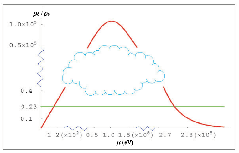
Figure 1: The dilaton mass density $\rho(\mu)$ versus the dilaton mass $\mu$, obtained with $g_{1}\simeq g_{2}\simeq 1$.

Note that the smaller mass $\mu_{1}$ is insensitive to the values of the coupling constants, while the larger mass $\mu_{2}$ increases as the coupling constants decrease. On the other hand, the life-time $\tau_{1}$ is sensitive to the values of the coupling constants, while the life-time $\tau_{2}$ remains of the same order for all values of the coupling constants.

With $g_{1}\simeq g_{2}\simeq 1$ we can plot the dilaton density $\rho(\mu)$ against its mass $\mu$, which is shown in Fig.1. Note that $\rho(\mu)$ starts from zero and approaches to the maximum value of about $1.08\times 10^{5}\rho_{c}$ at $\mu\simeq 103~{}{\rm MeV}$, and again decreases to zero when $\mu$ goes to infinity. More importantly, $\rho(\mu)$ exceeds the dark matter density in the range $160~{}\textrm{eV}<\mu<276~{}\textrm{MeV}$. This means that when $\mu<160~{}\textrm{eV}$ or $\mu>276~{}\textrm{MeV}$, the dilaton undercloses the universe, but when $160~{}\textrm{eV}<\mu<276~{}\textrm{MeV}$ it overcloses the universe. This immediately rules out the dilaton with mass range $160~{}\textrm{eV}<\mu<276~{}\textrm{MeV}$. Moreover, we have two possible mass ranges which are of particular interest, $\mu_{1}\simeq 160~{}\textrm{eV}$ with life-time $\tau_{1}\simeq 3.84\times 10^{35}~{}\textrm{sec}$ and $\mu_{2}\simeq 276~{}\textrm{MeV}$ with life-time $\tau_{2}\simeq 3.29\times 10^{16}~{}\textrm{sec}$, which makes the dilaton the dominant matter of the universe.

$\rho_{d}/\rho_{c}$	$\mu_{1}$	$\tau_{1}$	$\mu_{2}$	$\tau_{2}$
$100~{}\%$	686 eV	$4.85\times 10^{33}$ sec	$270$ MeV	$3.65\times 10^{16}$ sec
$23~{}\%$	160 eV	$3.84\times 10^{35}$ sec	$276$ MeV	$3.29\times 10^{16}$ sec
$10~{}\%$	68.6 eV	$4.85\times 10^{36}$ sec	$280$ MeV	$3.12\times 10^{16}$ sec
$4~{}\%$	27.4 eV	$7.58\times 10^{37}$ sec	$284$ MeV	$2.93\times 10^{16}$ sec
$1~{}\%$	6.86 eV	$4.85\times 10^{39}$ sec	$291$ MeV	$2.68\times 10^{16}$ sec
$0.5~{}\%$	3.43 eV	$3.88\times 10^{40}$ sec	$294$ MeV	$2.59\times 10^{16}$ sec

Table 2: The dilaton mass and life-time versus the ratio $\rho_{d}/\rho_{c}$. Here the coupling constants $g_{1}$ and $g_{2}$ are set to be 1.

So far we have assumed that the dilaton occupies all of the dark matter, about 23% of the critical density $\rho_{c}$. But even when we loosen this constraint, we get similar result. Varying the ratio $\rho_{d}/\rho_{c}$ of the dilaton’s mass density to the critical density, we obtain the result shown in TABLE II with $g_{1}\simeq g_{2}\simeq 1$. The result shows that $\mu_{1}$ and $\tau_{1}$ are sensitive to the change of $\rho_{d}/\rho_{c}$, but $\mu_{2}$ and $\tau_{2}$ are not much affected by that. Moreover, the generic feature of the dilaton physics remains the same.

Now, we have to make sure that the dilaton mass should also satisfy the second constraint (37). To check this, notice that the $160~{}{\rm eV}$ dilaton is almost stable because $\tau_{1}\simeq 8.1\times 10^{17}~{}t_{0}$. So the energy density of the daughter particles must be negligible compared to the energy density of the dilaton. This means that this dilaton can easily satisfy the second constraint (37). On the other hand, most of the $276~{}{\rm MeV}$ dilaton should have decayed by now, because $\tau_{2}\simeq 6.9\times 10^{-2}~{}t_{0}$. Indeed only $0.5\times 10^{-6}$ of the heavy dilaton survives now. So the energy density of the daughter particles becomes much bigger than that of the dilaton. This means that the daughter particles from the heavy dilaton overclose the universe, and thus can not satisfy the second constraint. This effectively rules out the heavy dilaton. So only the $160~{}{\rm eV}$ dilaton can be accepted as the dark matter candidate.

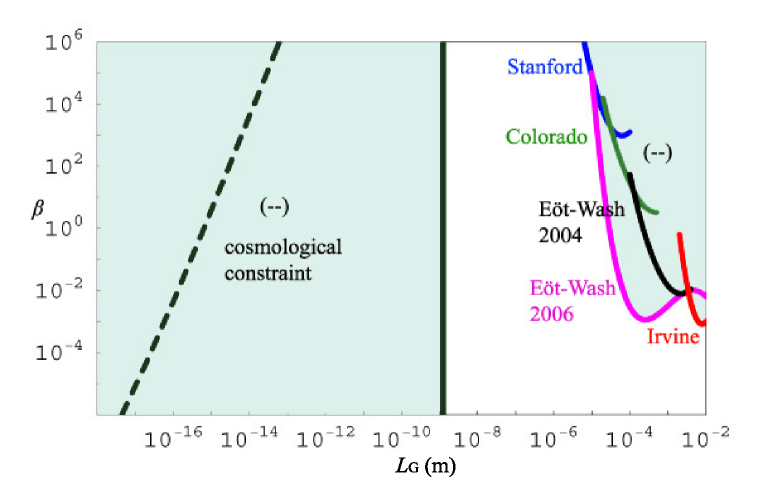
Figure 2: The possible scale $L_{G}=1/\mu$ of the internal space versus the relative fine structure constant $\beta=\alpha_{5}/\alpha_{g}$ of the fifth force in $(4+3)$-dimensional unification with $S^{3}$ compactification of the internal space. The colored region marked by (–) is the excluded region, and the dotted line represents the constraint of the heavy dilaton whose daughter particles overclose the universe.

The dark matter dilaton has the following characteristics. With the mass $\mu\simeq 160~{}\textrm{eV}$, the possible decay channels of the dilaton are the $\gamma\gamma$ and three $\nu\overline{\nu}$ processes. But with life-time $\tau\simeq 8.1\times 10^{17}~{}t_{0}$ this dilaton is almost stable. To see whether this can be hot or cold dark matter, we should estimate the free-streaming distance $\lambda_{FS}$ of the dilaton first. The dilaton in this case becomes nonrelativistic at $T_{NR}\simeq\mu/3\simeq 53.3~{}\textrm{eV}$ well before the matter-radiation equilibrium era $t_{EQ}\simeq 4.36\times 10^{10}(\Omega_{0}h^{2})^{-2}~{}\textrm{sec}\simeq 1.82\times 10^{11}~{}\textrm{sec}$. The time $t_{NR}$ when the dilaton becomes nonrelativistic is given by kol

$$t_{NR}\simeq 1.2\times 10^{7}\Bigg{(}\displaystyle\frac{\textrm{keV}}{\mu}\Bigg{)}^{2}\Bigg{(}\displaystyle\frac{T_{NR}}{T_{\gamma}}\Bigg{)}^{2}\textrm{sec}=1.2\times 10^{7}\Bigg{(}\displaystyle\frac{\textrm{keV}}{\mu}\Bigg{)}^{2}\Bigg{(}\displaystyle\frac{g_{*NR}}{g_{*D}}\Bigg{)}^{2/3}\textrm{sec},$$

$$\displaystyle\frac{t_{EQ}}{t_{NR}}=\Big{[}\displaystyle\frac{\mu/\textrm{eV}}{17(\Omega_{0}h^{2})(T_{NR}/T_{\gamma})}\Big{]}^{2},$$ (39)

where $T_{\gamma}$ is the temperature of the photon at $t_{NR}$, $g_{*NR}$ is the total relativistic degrees of freedom when the dilaton becomes non-relativistic. So the free-streaming distance $\lambda_{FS}$ is given by cqg98 ; kol ,

$$\lambda_{FS}\simeq 0.2\textrm{Mpc}\bigg{(}\displaystyle\frac{\mu}{\textrm{keV}}\bigg{)}^{-1}\bigg{(}\displaystyle\frac{T_{NR}}{T_{\gamma}}\bigg{)}~{}\Big{[}\textrm{ln}\bigg{(}\displaystyle\frac{t_{EQ}}{t_{NR}}\bigg{)}+2\Big{]}$$

$$=0.2\textrm{Mpc}\bigg{(}\displaystyle\frac{\mu}{\textrm{keV}}\bigg{)}^{-1}\bigg{(}\displaystyle\frac{g_{*NR}}{g_{*D}}\bigg{)}^{1/3}~{}\Big{[}\textrm{ln}\bigg{(}\displaystyle\frac{t_{EQ}}{t_{NR}}\bigg{)}+2\Big{]}.$$ (40)

Now, with $g_{*D}\simeq~{}106.75$ and $g_{*NR}\simeq 3.91$ we get $t_{NR}\simeq 5.17\times 10^{7}~{}\textrm{sec}$ and $\lambda_{FS}\simeq 4.2~{}\textrm{Mpc}$. Comparing the latter with the typical structure formation scale $\lambda_{EQ}\simeq 13(\Omega_{0}h^{2})^{-1}\simeq 18.6~{}\textrm{Mpc}$, we may conclude that the 160 keV dilaton becomes a warm dark matter.

In comparison the dilaton with mass $\mu\simeq 276~{}\textrm{MeV}$ becomes non-relativistic at $T_{NR}\simeq\mu/3\simeq 92~{}\textrm{MeV}$. The decay channels available here are $\gamma\gamma$, $\nu\overline{\nu}$, $e^{+}e^{-}$, $\mu^{+}\mu^{-}$ processes. Among them, only the $\mu^{+}\mu^{-}$ process is comparable to the $\gamma\gamma$ process since the mass of the muon $m_{\mu}\simeq 106~{}\textrm{MeV}$ is around $0.32\times\mu_{2}$. With life-time $\tau\simeq 6.9\times 10^{-2}~{}t_{0}$, only a fraction of the dilatons have survived up to now. In this case we have $g_{*NR}\simeq 19.5$ since only photon, three neutrinos, electron, and muon could be in thermal equilibrium at $t=t_{NR}$. With this value, we get $t_{NR}\simeq 5.07\times 10^{-5}~{}\textrm{sec}$ and $\lambda_{FS}\simeq 1.55\times 10^{-5}~{}\textrm{Mpc}\ll\lambda_{EQ}\simeq 18.6~{}\textrm{Mpc}$. So this dilaton could have been an excellent candidate for cold dark matter. But of course, this dilaton is not acceptable because the daughter particles overclose the universe.

As we have shown there are two constraints on the dilaton mass, the experimental constraint from the fifth force and the theoretical constraint from cosmology. Clearly these constraints restricts the allowed scale of the internal space. Putting the two constraints together we obtain Fig.2, which shows the allowed regions of the scale of the internal space versus the relative fine structure constant $\beta=\alpha_{5}/\alpha_{g}$ of the fifth force. Notice that the cosmological constraint tells that the scale of the internal space can not be smaller than $10^{-9}~{}{\rm m}$.

V Dilaton Detection Experiment

So far, we have tried to estimate the dilaton mass based on the conjecture that the dilaton is the dark matter of the universe. Now an important question is how to detect the relic dilaton and confirm such conjecture. Clearly one could try to establish the existence of the dilaton measuring the dilatonic fifth force grg91 ; exp1 . But the above analysis implies that, if indeed the dilaton is the dark matter of the universe, it’s detection by the fifth force experiments would be almost impossible because such dilaton generates an extremely short ranged fifth force.

In this section we propose a totally different type of experiment based on two photon decay of the relic dilaton. Of course, one might try to detect the two photon decay of the relic dilaton directly, searching for the mono-energetic x-ray signals from the sky cqg98 . Here we propose another type of experiment, a Sikivie-type experiment which detects the dilaton conversion to one photon in strong electromagnetic background. In this type of experiment the dilaton conversion rate can be greatly enhanced by two factors, first by the strong electromagnetic background and secondly by the large dilaton density of halo. It is clear that the conversion rate is enhanced by the strong background, because the conversion amplitude is proportional to the background field strength. Moreover, just as in the axion detection experiment, we can assume that our galaxy halo is made of the relic dilaton if the dark matter is the dilaton. In this case the conversion rate will be enhanced by a factor $10^{5}$, because the average energy density of the relic dilaton $0.23\times 10.5~{}h^{2}~{}\textrm{keV cm}^{-3}\simeq 1.18~{}\textrm{keV cm}^{-3}$ in the present universe can be replaced by the galaxy halo density $\rho_{halo}\simeq 0.3~{}\mathrm{GeVcm^{-3}}$ asz . In the following we estimate the power of dilaton conversion to one photon in strong magnetic background, assuming that our galaxy halo is made of dilaton.

Consider a rectangular cavity with three edges $L_{x},~{}L_{y},~{}L_{z}$ and volume $V=L_{x}L_{y}L_{z}$ made of a perfect conductor, which has a strong magnetic background $\vec{B}_{ext}(\vec{x})=B_{ext}(\vec{x})~{}\hat{z}$ in the z-direction inside, and consider the halo dilaton conversion in the cavity described by the interaction

$$\mathcal{L}_{\sigma\gamma\gamma}=-\alpha_{1}\hat{\sigma}F_{\mu\nu}^{2}=2\alpha_{1}\hat{\sigma}(\vec{E}^{2}-\vec{B}^{2}),~{}~{}~{}~{}~{}~{}\alpha_{1}=\displaystyle\frac{1}{4}g_{1}\sqrt{16\pi G}.$$ (41)

In this case the induced photon is described by TE mode (the magnetic wave) $\vec{B}(\vec{x})=B(\vec{x})~{}\hat{z}$, and the differential cross-section $d\sigma$ of the dilaton conversion in the cavity is given by

$$d\sigma_{\vec{k},\lambda}=2\pi\delta(k^{0}-p^{0})\displaystyle\frac{1}{2p^{0}v}\displaystyle\frac{d^{3}\vec{k}}{(2\pi)^{3}2k^{0}}|M|^{2},$$

$$M=-i4\alpha_{1}\vec{B}(\vec{x})\cdot\vec{B}_{ext}(\vec{q})=-i4\alpha_{1}k^{0}(\hat{\epsilon}(\vec{k},\lambda)\times\hat{k})\cdot\vec{B}_{ext}(\vec{q}),$$ (42)

where $p^{\mu}$ and $k^{\mu}$ are the 4-momenta of the dilaton and the induced photon, $M$ is the Feynman reduced matrix element, $\hat{\epsilon}(\vec{k},\lambda=\pm 1)$ and $\hat{k}$ are the 3-dimensional photon polarization vector and the unit vector in the direction of the photon momentum $\vec{k}$, $\vec{q}=\vec{k}-\vec{p}$ is the spatial momentum transfer, and $\vec{B}_{ext}(\vec{q})$ is the Fourier transform of $\vec{B}_{ext}(\vec{x})$. Note that in the classical background only energy is conserved, and the $\delta(k^{0}-p^{0})$ term represents this fact. Then the total cross-section $\sigma$ in the continuum limit is given as follows,

$$\sigma=\displaystyle\frac{}{}\sum_{\lambda=\pm 1}2\pi\int d^{3}\vec{k}~{}\delta(k^{0}-p^{0})\displaystyle\frac{1}{2p^{0}v}\displaystyle\frac{1}{(2\pi)^{3}2k^{0}}|M|^{2}$$

$$=\displaystyle\frac{\alpha_{1}^{2}}{\pi^{2}v}\sum_{\lambda=\pm 1}\int d^{3}\vec{k}\delta(k^{0}-p^{0})|\hat{B}(\vec{k},\lambda)\cdot\vec{B}_{ext}(\vec{q})|^{2},$$ (43)

where $\hat{B}(k,\lambda)=\hat{\epsilon}(\vec{k},\lambda)\times\hat{k}$ is the unit vector in the direction of the induced magnetic field $\vec{B}$.

Let the wave vector of the photon be $\vec{k}=(n_{x}\pi/L_{x},~{}n_{y}\pi/L_{y},~{}n_{z}\pi/L_{z})$ where $(n_{x},~{}n_{y},~{}n_{z})$ are arbitrary integers. For TE modes, the boundary condition

$$B~{}(z=0,L_{z})=0~{},~{}~{}\displaystyle\frac{\partial B}{\partial x}(x=0,L_{x})=0~{},~{}~{}\displaystyle\frac{\partial B}{\partial y}(y=0,L_{y})=0,$$ (44)

requires the induced magnetic field to assume the form

$$B=A\cos\bigg{(}\displaystyle\frac{n_{x}\pi x}{L_{x}}\bigg{)}\cos\bigg{(}\displaystyle\frac{n_{y}\pi y}{L_{y}}\bigg{)}\sin\bigg{(}\displaystyle\frac{n_{z}\pi z}{L_{z}}\bigg{)},$$ (45)

where $A$ is a normalization constant. Notice that $n_{x}$ and $n_{y}$ cannot be zero simultaneously, and $n_{z}$ must be a non-zero integer jac .

Now, we have

$$\displaystyle\frac{}{}\sum_{\lambda=\pm 1}|\hat{B}(\vec{k},\lambda)\cdot\vec{B}_{ext}(\vec{q})|^{2}=|\hat{k}\times B_{ext}(\vec{q})\hat{z}|^{2}=\displaystyle\frac{k_{x}^{2}+k_{y}^{2}}{{(k^{0})}^{2}}|B_{ext}(\vec{q})|^{2},$$

$$\vec{B}_{ext}(\vec{q})=\displaystyle\frac{}{}\int_{V}e^{i\vec{q}\cdot\vec{x}}\vec{B}_{ext}(\vec{x})~{}d^{3}\vec{x}=\displaystyle\frac{}{}\int_{V}e^{i\vec{q}\cdot\vec{x}}B_{ext}(\vec{x})\hat{z}~{}d^{3}\vec{x}=B_{ext}(\vec{q})\hat{z},$$ (46)

so that, changing the integration into summation as follows

$$d^{3}\vec{k} = dk_{x}dk_{y}dk_{z}=\frac{\pi}{L_{x}}\frac{\pi}{L_{y}}\frac{\pi}{L_{z}}dn_{x}dn_{y}dn_{z}=\frac{\pi^{3}}{V},$$ (47)

we get the following cross-section

$$\sigma = \sum_{\vec{k}}\frac{\pi\alpha^{2}}{Vv}\frac{(k_{x}^{2}+k_{y}^{2})}{(k^{0})^{2}}\delta(k^{0}-p^{0})|B_{ext}(\vec{q})|^{2}.$$ (48)

To proceed, we let

$$\vec{B}_{ext}(\vec{x})=B_{0}\cos(Qx)\hat{z},$$ (49)

and approximate $\vec{q}=(\vec{k}-\vec{p})\sim\vec{k}$ since the incoming halo dilaton is highly non-relativistic (with $v\sim 10^{-3}c)$ asz . In this case we have

$$|B_{ext}(\vec{q})|^{2}=|\displaystyle\frac{}{}\int_{V}d^{3}\vec{x}e^{i\vec{q}\cdot\vec{x}}B_{0}\cos(Qx)|^{2}$$

$$=B_{0}^{2}L_{x}^{2}L_{y}^{2}L_{z}^{2}\displaystyle\frac{\sin^{2}(\displaystyle\frac{k_{y}L_{y}}{2})}{(\displaystyle\frac{k_{y}L_{y}}{2})^{2}}\displaystyle\frac{\sin^{2}(\displaystyle\frac{k_{z}L_{z}}{2})}{(\displaystyle\frac{k_{z}L_{z}}{2})^{2}}\times\displaystyle\frac{1}{4}\Big{(}\Big{[}\displaystyle\frac{\sin(k_{x}-Q)L_{x}}{(k_{x}-Q)L_{x}}+\displaystyle\frac{\sin(k_{x}+Q)L_{x}}{(k_{x}+Q)L_{x}}\Big{]}^{2}$$

$$+\Big{[}\displaystyle\frac{1-\cos(k_{x}-Q)L_{x}}{(k_{x}-Q)L_{x}}+\displaystyle\frac{1-\cos(k_{x}+Q)L_{x}}{(k_{x}+Q)L_{x}}\Big{]}^{2}\Big{)}.$$ (50)

As we can see, $|B_{ext}(\vec{q})|^{2}$ has the maximum value

$$|B_{ext}(\vec{q})|^{2}_{max}=\frac{B_{0}^{2}L_{x}^{2}L_{y}^{2}L_{z}^{2}}{\pi^{2}}~{},$$ (51)

when

$$k_{x}=\pm Q,~{}k_{z}L_{z}=\pm\pi~{},~{}k_{y}L_{y}=0~{}.$$ (52)

Note that $|B_{ext}(\vec{q})|^{2}_{max}$ would be highly suppressed without the external sinusoidal background, which is why we choose the sinusoidal external magnetic field (49).

We are interested in the dilaton with the mass range $\mu\gtrsim 0.1~{}\textrm{keV}$ whose Compton wave-length is of order smaller than $2\times 10^{-7}~{}\textrm{cm}$. Considering the typical detector length scale $L_{x},~{}L_{y},~{}L_{z}\simeq 1~{}\mathrm{m}$ and $(k^{0})^{2}=k_{x}^{2}+k_{y}^{2}+k_{z}^{2}\simeq\mu^{2}$, we have $k_{x}\simeq k^{0}\gg{\rm Max}~{}(k_{y},k_{z})$ since $\mu L_{x},~{}\mu L_{y}\gg 1$ in the resonance case. Thus we can use the following approximation

$$k^{0}dk^{0}=k_{x}dk_{x}+k_{y}dk_{y}+k_{z}dk_{z}\simeq k_{x}dk_{x}\Rightarrow dk^{0}=\frac{k_{x}}{k^{0}}dk_{x}\simeq dk_{x}~{}.$$ (53)

On the other hand, the number of additional modes due to the differential spread $dk^{0}$ around $k^{0}=p^{0}$ is

$$dn_{x}=\displaystyle\frac{L_{x}}{\pi}dk_{x}\simeq\displaystyle\frac{L_{x}}{\pi}dk^{0},~{}~{}~{}~{}~{}\delta(k^{0}-p^{0})dn_{x}=\displaystyle\frac{L_{x}}{\pi}~{}.$$ (54)

Combining these relations, we finally obtain

$$\sigma=\displaystyle\frac{}{}\sum_{\vec{k}}\displaystyle\frac{\pi\alpha_{1}^{2}}{Vv}\displaystyle\frac{(k_{x}^{2}+k_{y}^{2})}{(k^{0})^{2}}\delta(k^{0}-p^{0})|B_{ext}(\vec{q})|^{2}\simeq\displaystyle\frac{4\pi\alpha_{1}^{2}}{Vv}\displaystyle\frac{(k^{0})^{2}}{(k^{0})^{2}}\delta(k^{0}-p^{0})dn_{x}\times|B_{ext}(\vec{q})|^{2}_{max}$$

$$=\displaystyle\frac{16\pi\alpha_{1}^{2}}{Vv}\displaystyle\frac{L_{x}}{\pi}\times|B_{ext}(\vec{q})|^{2}_{max}=\displaystyle\frac{4\alpha_{1}^{2}}{\pi^{2}Vv}B_{0}^{2}L_{x}^{2}L_{y}^{2}L_{z}^{2}L_{x}=\displaystyle\frac{4\alpha_{1}^{2}}{\pi^{2}v}B_{0}^{2}VL_{x},$$ (55)

and the following detection power $P$

$$P=\mu~{}n_{d}v\sigma=\Bigg{(}\displaystyle\frac{4\alpha_{1}^{2}}{{\pi}^{2}}\Bigg{)}\rho_{d}B_{0}^{2}L_{x}V,$$ (56)

where $n_{d}$ is the dilaton number density and $\rho_{d}$ is the dilaton energy density. Notice that the detection power depends on the energy density, not the mass, of dilaton.

This agrees with that of the axion detection power except for the numerical factor of order unity which comes from the different axion-photon coupling constant. In the case of the axion, the axion-photon interaction Lagrangian and axion detection power are given as follows sik ,

$$\mathcal{L}_{a\gamma\gamma}=-\alpha_{\gamma}~{}a~{}F_{\mu\nu}\tilde{F}^{\mu\nu}=4\alpha_{\gamma}~{}a~{}\vec{E}\cdot\vec{B},$$

$$P_{a}=2\alpha_{\gamma}^{2}\rho_{a}B_{0}^{2}L_{x}V.$$ (57)

As we have mentioned there are two types of axion, the popular axion from strong interaction and the gravitational axion proposed as a pseudoscalar graviton pec ; ni . The difference is that for the popular axion the coupling constant $\alpha_{\gamma}$ is given by $g_{\gamma}\alpha/4\pi f_{a}$, where $g_{\gamma}$ is a model-dependent dimensionless coupling constant of order one, $\alpha$ is the electromagnetic fine-structure constant, and $f_{a}$ is the $U_{PQ}(1)$ symmetry breaking scale. But for the gravitational axion $\alpha_{\gamma}$ is similar to our $\alpha_{1}$ because this axion is the pseudoscalar partner of the dilaton. Other than this they are virtually identical.

We can compare the axion detection power with the dilaton detection power. Consider the popular axion first. Since $f_{a}$ is related to the axion mass $m_{a}$ by $m_{a}\simeq 6~{}\mathrm{eV}\times 10^{6}~{}\mathrm{GeV}/f_{a}$, and the educated guess of the axion mass is around $10^{-6}~{}\mathrm{eV}$ or so, we have $f_{a}\simeq 6\times 10^{12}~{}{\rm GeV}$ sik ; asz . So we have

$$\displaystyle\frac{P}{P_{a}}\simeq 1.9\times 10^{6}\times\big{(}\displaystyle\frac{g_{1}}{g_{\gamma}}\big{)}^{2}\big{(}\displaystyle\frac{f_{a}}{m_{p}}\big{)}^{2}\simeq 4.7\times 10^{-7}.$$ (58)

This is a small number, but this is because $\alpha_{1}$ is smaller than $\alpha_{\gamma}$ due to the fact that $f_{a}$ is much bigger than the Planck mass. Indeed, with $\rho_{d}\simeq\rho_{halo}\simeq 0.5\times 10^{-24}~{}\mathrm{g/cm^{3}}\simeq 0.3~{}\mathrm{GeV/cm^{3}}$ and $B_{0}=10~{}\mathrm{Tesla}$, $L_{x}=L_{y}=L_{z}\simeq 1~{}\mathrm{m}$, we get the dilaton detection power $P\simeq 1.42\times 10^{-31}~{}\textrm{W}$ with $g_{1}\simeq 1$. This is $10^{-5}$ times smaller than the axion detection power in current experiments sik ; asz . For the gravitation axion, however, we expect $\alpha_{1}\simeq\alpha_{\gamma}$ so that $P_{a}$ becomes as small as $P$. So in this case the axion detection power becomes smaller than the popular axion detection power, and becomes comparable to the dilaton detection power.

Notice that, due to the pseudoscalar coupling, the axion produces TM modes (the electric wave) rather than TE modes. Another notable difference between the dilaton and the axion is that for the dilaton the photon polarization is perpendicular to the external magnetic field, whereas for the axion the photon polarization is parallel to the external magnetic field.

Now, a few remarks are in order. First, the above result holds when we have the resonance, $Q\simeq\mu$. But it seems very difficult to make static magnetic field of wavelength of order $\mu^{-1}\lesssim 10^{-7}~{}\mathrm{cm}$ with the current technology. However we may be able to set up x-ray range electromagnetic waves with $\omega_{ext}=Q\simeq\mu$. In that case, the only change needed is to replace $\delta(k^{0}-p^{0})$ by $\delta(k^{0}-p^{0}\pm p^{0})$ in the above calculation, which will make the detection power $P$ twice as big. Second, the dilaton detection power appears too small to be considered realistic at present. On the other hand, we notice that the relevant technologies are developing fast asz , so that it may be possible to detect the halo dilaton in the near future. Third, we have used the magnetic background in the above calculation. With an electric background the detection power would have been proportional to the electric field energy density. In terms of the field energy density, 1 Tesla corresponds to $300~{}\mathrm{MV/m}$ since $E=cB$ in the MKS unit system. But the strongest magnetic field and electric fields currently available are around 50 Tesla and 40 MV/m MEmax , respectively. So at present a magnetic background can give us larger detection power. Moreover, in the air the electric breakdown happens when the electric field is about 3 MV/m. This is why we have used the magnetic background in our calculation. And this is why one hardly uses an electric background in particle creation or annihilation experiments in laboratories.

VI Discussion

The Newton’s constant in Einstein’s theory has always been a mystery. The Einstein’s theory has a dimensional coupling constant, the Newton’s constant, because the source of gravity is the energy-momentum tensor. The problem is that in mass scale, this coupling constant is absurdly bigger than the ordinary elementary particle mass scale. In this paper we have shown how the dilaton from higher-dimensional unification can naturally resolve this mystery. First, the dilaton makes the Newton’s constant a space-time dependent parameter. This changes the hierarchy problem from a fundamental problem to a space-time dependent artifact. Moreover, it reduces the Planck mass down to the ordinary mass scale when the internal space becomes larger than the Planck size. This is because the dilaton mass is fixed by the curvature of the internal space. So it can be small even though the unit of the curvature is set by the Planck mass. When the internal space becomes larger, it becomes flatter and the curvature becomes smaller. This means that the dilaton mass can be much smaller than the Planck mass when the size of the internal space is big enough. This is how the Kaluza-Klein dilaton resolves the hierarchy problem cho .

As the scalar graviton the dilaton couples to all matters, so that it creates the fifth force which modifies Einstein’s gravity. This is why the fifth force experiments have been used to detect the dilaton. On the other hand the dilaton coupling to matter fields is very weak. This means that the dilaton can easily survive to present universe. This makes the dilaton an excellent candidate of dark matter. Our analysis tells that there is practically only one mass range, $\mu\simeq 160~{}{\rm eV}$, for which the dilaton can be the dark matter. This cosmological constraint of dilaton mass implies that detecting the dilaton by the fifth force experiments would be futile, because the fifth force is too short ranged to be detected in the near future.

In this paper we have proposed a totally different type of experiment to detect the dilaton, based on the dilaton photon conversion in strong magnetic background. Although the detection power of dilaton is still very small, we hope that this type of experiment could help us to detect the dilaton.

ACKNOWLEDGEMENT

The work is supported in part by the BSR Program (Grant KRF-2007-314-C00055) of Korea Research Foundation and by the ABRL Program (Grant R14-2003-012-01002-0) of Korea Science and Engineering Foundation.

References

- (1) Y.M. Cho, Phys. Rev. D 41, 2462 (1990); Y.M. Cho and J.H. Yoon, Phys. Rev. D 47, 3465 (1993). See also, Y.M. Cho, in Proceedings of XXth Yamada Conference on Big Bang, Active Galactic Nuclei, and Supernovae, edited by S. Hayakawa and K. Sato (University Academy, Tokyo) 1988.
- (2) P. Sikivie, Phys. Rev. Lett. 51, 16 (1983); Phys. Rev. D 32, 11 (1985); P. Sikivie, D. Tanner, and Y. Wang, Phys. Rev. D 50, 4744 (1994).
- (3) Y.M. Cho, J. Math. Phys. 16, 2029 (1975); Y.M. Cho and P.G.O. Freund, Phys. Rev. D 12, 1711 (1975); Y.M. Cho and P.S. Jang, Phys. Rev. D 12, 3138 (1975).
- (4) See e.g., M. Duff, B. Nielson, and C. Pope, Phys. Rep. 130, 1 (1986).
- (5) See e.g., M. Green, J. Schwartz, and E. Witten, Superstring theory, Vol. 2 (Cambridge University Press) 1987.
- (6) R. Peccei and H. Quinn, Phys. Rev. Lett. 38, 1440 (1977); Phys. Rev. D 16, 1791 (1977).
- (7) S. Weinberg, Phys. Rev. Lett. 40, 233 (1978); F. Wilczek, Phys. Rev. Lett. 40, 279 (1978).
- (8) W.T. Ni, Phys. Rev. Lett. 38, 301 (1977).
- (9) S. Asztalos et al., J. Astrophys. 30, 571 (2002); S. Asztalos et al., Ann. Rev. Nucl. Part. Sci. 56, 293 (2006). See also R. Bradly et al., Rev. Mod. Phys. 75, 3 (2003).
- (10) Y.M. Cho, Phys. Rev. D 35, 2628 (1987); Phys. Lett. B 199, 358 (1987).
- (11) Y.M. Cho and D.H. Park, Gen. Rel. Grav. 23, 741 (1991).
- (12) Y.M. Cho and Y.Y. Keum, Class. Quant. Grav. 15, 907 (1998).
- (13) P. Jordan, Ann. Phys. (Leibzig) 1, 218 (1947); W. Pauli, in Schwerkraft und Weltall (F.Vieweg und Sohn, Braunschweig) 1955; C. Brans and R. Dicke, Phys. Rev. 124, 921 (1961).
- (14) Y.M. Cho, Phys. Rev. Lett. 68, 21 (1992).
- (15) E. Fishbach et al., Phys. Rev. Lett. 56, 3 (1986); C. Hoyle et al., Phys. Rev. Lett. 86, 1418 (2001).
- (16) D. Kapner et al., Phys. Rev. Lett. 98, 021101 (2007); E. Adelberger et al., Phys. Rev. Lett. 98, 131104 (2007).
- (17) P.A.M. Dirac, Nature (London)136, 323 (1937).
- (18) N. Arkani-Hamed, S. Dimopoulos, and G. Dvali, Phys. Lett. B 429, 263 (1998); N. Arkani-Hamed, I. Antoniadis, S. Dimopoulos, and G. Dvali, Phys. Lett. B 436, 257 (1998).
- (19) I. Antoniadis, S. Dimopoulos, and G. Dvali, Nucl. Phys. B 516, 70 (1998); Phys. Rev. Lett 84, 586 (2000).
- (20) The dimensional reduction by isometry as the only logically viable dimensional reduction has also been emphasized recently by Penrose. See R. Penrose, The Road to Reality : A Complete Guide to The Laws of The Universe, A.A. Knopf, 2005.
- (21) J. Khoury and A. Weltman, Phys. Rev. Lett. 93, 171104 (2004).
- (22) W. Greiner and J. Reinhardt, Quantum Electrodynamics (Springer, Berlin) 1994.
- (23) E. Kolb and M. Turner, The Early Universe (Addison-Wesley, New York) 1993.
- (24) M. Tegmark, A. Aguirre, M. Rees and F. Wilczek, Phys. Rev. D 73, 023505 (2006).
- (25) J.D. Jackson, Classical Electrodynamics (Wiley, New York) 1975.
- (26) D. Lai, astro-ph/0009333; L. Lilje et al., physics/0401141.
- (27) Y.M.Cho, J.H. Kim, S.W. Kim, and J.H. Yoon, hep-ph/0708.2590, to be bublished.