Mitigating the effects of measurement noise on Granger causality

Abstract

Computing Granger causal relations among bivariate experimentally observed time series has received increasing attention over the past few years. Such causal relations, if correctly estimated, can yield significant insights into the dynamical organization of the system being investigated. Since experimental measurements are inevitably contaminated by noise, it is thus important to understand the effects of such noise on Granger causality estimation. The first goal of this paper is to provide an analytical and numerical analysis of this problem. Specifically, we show that, due to noise contamination, (1) spurious causality between two measured variables can arise and (2) true causality can be suppressed. The second goal of the paper is to provide a denoising strategy to mitigate this problem. Specifically, we propose a denoising algorithm based on the combined use of the Kalman filter theory and the Expectation-Maximization (EM) algorithm. Numerical examples are used to demonstrate the effectiveness of the denoising approach.

I Introduction

Granger causality Granger has become the method of choice to determine whether and how two time series exert causal influences on each other. In this method one starts by modeling simultaneously acquired time series as coming from a multivariate or vector autoregressive (VAR) stochastic process. One time series is said to have a causal influence on the other if the residual error in the autoregressive model of the second time series (at a given point of time) is reduced by incorporating past measurements from the first. This method and related methods have found applications in a wide variety of fields including physics Blinowska ; Marinazzo ; Verdes ; Rosenblum ; Hu ; Xu , economics Granger ; Thornton ; Hall ; Hiemstra and neuroscience Ding ; Ding2 . Its nonlinear extension has recently appeared in Chen and has been applied to study problems in condensed matter physics Rajesh .

The statistical basis of Granger causality estimation is linear regression. It is known that regression analysis is sensitive to the impact of measurement noise wayne . Given the inevitable occurrence of such noise in experimental time series, it is imperative that we determine whether and how such added noise can adversely affect Granger causality estimation. Previous studies Newbold have suggested that such adverse effects can indeed occur. In this paper, we make further progress by obtaining analytical expressions that explicitly demonstrate how the interplay between measurement noise and system parameters affects Granger causality estimation. Moreover, we show how this deleterious effect of noise can be reduced by a denoising method, which is based on the Kalman filter theory and the Expectation-Maximization (EM) algorithm. We refer to our denoising algorithm as the KEM (Kalman EM) denoising algorithm.

The organization of this paper is as follows. In Section 2, we start by introducing an alternative formulation of Granger causality Pierce and proceed to outline a framework within which the effects of added (measurement) noise on the estimation of directional influences in bivariate autoregressive processes can be addressed. To simplify matters, we then consider a bivariate first order autoregressive (AR(1)) process in Section 3. Here explicit expressions for the effect of noise on Granger causality are derived. These expressions allow us to show that, for two time series that are unidirectionally coupled, spurious causality can arise when noise is added to the driving time series and true causality can be suppressed by the presence of noise in either time series. The theoretical results are illustrated by numerical simulations. In Section 4, we briefly introduce the KEM denoising algorithm and apply it to the example considered in Section 3. Our results show that the KEM algorithm can mitigate the effects of noise and restore the true causal relations between the two time series. In section 5, we consider a coupled neuron model which produces time series that closely resemble that recorded in neural systems. The effect of noise on Granger causality and the effectiveness of the KEM algorithm in mitigating the noise effect are illustrated numerically. Our conclusions are given in Section 6.

II Theoretical Framework

Consider two time series $X(t)$ and $Y(t)$. To compute Granger causality, we model them as a combined bivariate autoregressive process of order $p$. In what follows, the model order $p$ is assumed to be known, since this aspect is not central to our analysis. The bivariate autoregressive model can then be represented as:

$$\sum_{k=0}^{p}[a_{k}X(t-k)+b_{k}Y(t-k)]=E_{1}(t),$$ (1)

$$\sum_{k=0}^{p}[c_{k}X(t-k)+d_{k}Y(t-k)]=E_{2}(t),$$ (2)

where $a_{k}$, $b_{k}$, $c_{k}$, and $d_{k}$ are the AR coefficients and $E_{i}(t)$ are the temporally uncorrelated residual errors.

For our purposes, it is more convenient to rewrite the above bivariate process as two univariate processes (this can always be done according to Pierce ):

$$P_{1}(B)X(t)={\xi(t)};\ \ \ P_{2}(B)Y(t)={\eta(t)},$$ (3)

where $B$ is the lag operator defined as $B^{k}X(t)=X(t-k)$ and $P_{1}$ and $P_{2}$ are polynomials (of possibly infinite order) in the lag operator $B$. It should be noted that the new noise terms $\xi(t)$ and $\eta(t)$ are no longer uncorrelated. Let $\gamma_{12}(k)$ denote the covariance at lag $k$ between these two noises.

$${\gamma_{12}(k)}\equiv{\rm cov}({\xi(t))},{\eta(t-k)})~{}~{}~{}~{}~{}~{}~{}{k=...,-1,0,1...}\ .$$ (4)

A theorem by Pierce and Haugh Pierce states that ${Y(t)}$ causes ${X(t)}$ in Granger sense if and only if

$${\gamma_{12}(k)\neq 0}~{}\rm{for~{}some}~{}k>0.$$ (5)

Similarly ${X(t)}$ causes ${Y(t)}$ if and only if ${\gamma_{12}(k)\neq 0}$ for some $k<0$.

Now we add measurement noises $\xi^{\prime}(t)$ and $\eta^{\prime}(t)$ to $X(t)$ and $Y(t)$ respectively:

$${X^{(c)}(t)}={X(t)}+{\xi^{\prime}(t)},$$ (6)

$${Y^{(c)}(t)}={Y(t)}+{\eta^{\prime}(t)}.$$ (7)

Here ${\xi^{\prime}(t)}$, ${\eta^{\prime}(t)}$ are uncorrelated white noises that are uncorrelated with ${X(t)},{Y(t)},{\xi(t)}$ and ${\eta(t)}.$ Following Newbold Newbold , the above equations can be rewritten as

$$P_{1}(B){X}^{(c)}(t)=P_{1}(B){X}(t)+P_{1}(B){\xi}^{\prime}(t),$$ (8)

$$P_{2}(B){Y}^{(c)}(t)=P_{2}(B){Y}(t)+P_{2}(B){\eta}^{\prime}(t).$$ (9)

Using Eq. (3) we get

$$P_{1}(B){X}^{(c)}(t)={\xi}(t)+P_{1}(B){\xi}^{\prime}(t),$$ (10)

$$P_{2}(B){Y}^{(c)}(t)={\eta}(t)+P_{2}(B){\eta}^{\prime}(t).$$ (11)

Following the procedure in Granger and Morris Morris , the linear combination of white noise processes on the right hand sides can be rewritten in terms of invertible moving average processes Maravall :

$${\xi}(t)+P_{1}(B){\xi}^{\prime}(t)=P_{3}(B){\xi}^{(c)}(t),$$ (12)

$${\eta}(t)+P_{2}(B){\eta}^{\prime}(t)=P_{4}(B){\eta}^{(c)}(t),$$ (13)

where ${\xi^{(c)}}$ and ${\eta^{(c)}}$ are again uncorrelated white noise processes. Thus we get

$$P_{3}^{-1}(B)P_{1}(B){X}^{(c)}(t)={\xi^{(c)}}(t),$$ (14)

$$P_{4}^{-1}(B)P_{2}(B){Y}^{(c)}(t)={\eta^{(c)}}(t).$$ (15)

This is again in the form of two univariate AR processes. Therefore the theorem of Pierce and Haugh can be applied to yield the result that the noisy signal ${Y^{(c)}(t)}$ causes ${X^{(c)}(t)}$ in Granger sense if and only if

$${\gamma_{12}^{(c)}(k)}\equiv{\rm cov}({\xi}^{(c)}(t),{\eta}^{(c)}(t-k))\neq 0,$$ (16)

for some ${k}>0.$ Similarly ${X^{(c)}(t)}$ cause ${Y^{(c)}(t)}$ if and only if

$$\gamma_{12}^{(c)}(k)\neq 0,$$ (17)

for some ${k<0}$.

We can relate $\gamma_{12}^{(c)}$ to $\gamma_{12}$ as follows. Consider the corresponding covariance generating functions (which are nothing but the $z$-transforms of the cross-covariances)

$$\bar{\gamma}_{12}(z) = \sum_{k=-\infty}^{\infty}\gamma_{12}(k)z^{k},$$ (18)

$$\bar{\gamma}_{12}^{(c)}(z) = \sum_{k=-\infty}^{\infty}\gamma_{12}^{(c)}(k)z^{k}.$$ (19)

We can show that Newbold

$$\bar{\gamma}_{12}^{(c)}(z)=P_{3}^{-1}(z)P_{4}^{-1}(z^{-1})\bar{\gamma}_{12}(z).$$ (20)

Even if ${\gamma_{12}(k)=0}$ for all $k<0$ (i.e. ${X}$ does not cause ${Y}$) it is possible that $\gamma_{12}^{(c)}(k)\neq 0$ for some negative $k$ because of the additional term $P_{3}^{-1}(z)P_{4}^{-1}(z^{-1})$ that has been introduced by the measurement noise. This gives rise to the spurious Granger causality, (${X}^{(c)}$ causes ${Y^{(c)}}$), which is a consequence of the added measurement noise.

III A Bivariate AR(1) Process

In the previous section, we demonstrated that measurement noise can affect Granger causality. But the treatment given was quite general in nature. In this section we specialize to a simple bivariate AR(1) process and obtain explicit expressions for the effect of noise on Granger causality.

Consider the following bivariate AR(1) process

$${X(t)} = a{X(t-1)}+b{Y(t-1)}+E_{1}(t),$$

$${Y(t)} = d{Y(t-1)}+E_{2}(t).$$ (21)

From the above expressions, it is clear that $Y$ drives $X$ for nonzero values of $b$ and $X$ does not drive $Y$ in this model. More specifically, we see that $Y$ at an earlier time $t-1$ affects $X$ at the current time $t$. There is no such corresponding influence of $X$ on $Y$.

When noises $\xi^{\prime}(t)$ and $\eta^{\prime}(t)$ with variances $\sigma_{\xi^{\prime}}^{2}$ and $\sigma_{\eta^{\prime}}^{2}$, respectively, are added to the data generated by Eq. (21), after some algebra (see Appendix for details), we find the following expressions for $P_{3}(B)$ and $P_{4}(B)$:

$$P_{3}(B)=1+a_{1}^{\prime}B+a_{2}^{\prime}B^{2};\ \ \ P_{4}(B)=1-d^{\ {}^{\prime}}B.$$ (22)

Here

$$d^{\ {}^{\prime}}=\frac{s{\pm{\sqrt{s^{2}-{4}}}}}{2},$$ (23)

where

$$s\equiv(\frac{1}{d}+d)+\frac{1}{d}\frac{{\sigma_{\eta}^{2}}}{{\sigma_{\eta^{\prime}}^{2}}}.$$ (24)

The expressions for $a_{1}^{\prime}$ and $a_{2}^{\prime}$ are very long and for our purposes it is sufficient to note that they go to zero as the added noise goes to zero (as expected). We see that $|s|>2$ for any value of $d$, ${\sigma_{\eta}^{2}}$ and ${\sigma_{\eta^{\prime}}^{2}}$. Therefore $\sqrt{S^{2}-{4}}$ and hence $d{\ {}^{\prime}}$ are well defined. We also have the following results:

a) As $|d|\rightarrow 0$, $|d^{\ {}^{\prime}}|<|d|\rightarrow 0$;

b) As $d\rightarrow 1$, $d^{\ {}^{\prime}}\rightarrow 1+\frac{{\sigma_{\eta}^{2}}}{2{\sigma_{\eta^{\prime}}^{2}}}-\frac{{\sigma_{\eta}^{2}}}{2{\sigma_{\eta^{\prime}}^{2}}}\sqrt{1+4/\frac{{\sigma_{\eta}^{2}}}{{\sigma_{\eta^{\prime}}^{2}}}}$;

c) As the ratio $\frac{{\sigma_{\eta}^{2}}}{{\sigma_{\eta^{\prime}}^{2}}}\rightarrow 0,d^{\ {}^{\prime}}\rightarrow d$;

d) As the ratio $\frac{{\sigma_{\eta}^{2}}}{{\sigma_{\eta^{\prime}}^{2}}}\rightarrow\infty,d^{\ {}^{\prime}}\rightarrow 0$.

Substituting the expressions for $P_{3}(B)$ and $P_{4}(B)$ in Eq. (20) we get

$$\bar{\gamma}_{12}^{(c)}(z)=(1+a_{1}^{{}^{\prime}}{z}+a_{2}^{{}^{\prime}}{z^{2}})^{-1}(1-d^{\ {}^{\prime}}z^{-1})^{-1}\bar{\gamma}_{12}(z).$$ (25)

We now expand both sides in powers of $z$:

$$\cdots+\gamma_{12}^{(c)}(-1)z^{-1}+\gamma_{12}^{(c)}(0)+\gamma_{12}^{(c)}(1)z+\cdots=(1-a_{1}^{{}^{\prime}}{z}+(a_{1}^{2}-a_{2}^{{}^{\prime}}){z^{2}}+\cdots)$$

$$\times(1+d^{\ {}^{\prime}}z^{-1}+d^{{}^{\prime}2}z^{-2}+\cdots)(\cdots+\gamma_{12}(-1)z^{-1}+\gamma_{12}(0)+\gamma_{12}(1)z+\cdots).$$ (26)

Collecting terms proportional to $z^{-1},z^{0},z^{1}$ etc., we obtain the following expressions for the cross covariances at lag -1, 0 and 1:

$$\gamma_{12}^{(c)}(-1) = d^{\ {}^{\prime}}(1-a_{1}{{}^{\prime}}d^{\ {}^{\prime}}+\ldots)(\gamma_{12}(0)+d^{\ {}^{\prime}}\gamma_{12}(1)+\ldots),$$ (27)

$$\gamma_{12}^{(c)}(0) = (1-a_{1}^{{}^{\prime}}d^{\ {}^{\prime}}+\ldots)(\gamma_{12}(0)+d^{\ {}^{\prime}}\gamma_{12}(1)+\ldots),$$ (28)

$$\gamma_{12}^{(c)}(1) = \gamma_{12}(1)-a_{1}^{{}^{\prime}}\gamma_{12}(0)-a_{1}^{{}^{\prime}}d^{\ {}^{\prime}}\gamma_{12}(1)+\ldots\ .$$ (29)

We observe that $\gamma_{12}^{(c)}(k)$ for $k<0$ (and in particular, $\gamma_{12}^{(c)}(-1)$) is no longer zero, implying that the $X^{(c)}$ drives $Y^{(c)}$, thus giving rise to a spurious causal direction. The spurious causality term $\gamma_{12}^{(c)}(-1)$ is proportional to $d^{\ {}^{\prime}}$. This can be shown to be true for all the other spurious terms $\gamma_{12}^{(c)}(k),\ k<-1$ as well. Hence they all go to zero if $d^{\ {}^{\prime}}\rightarrow 0$ (i.e. if ${Y}$ has no measurement noise). This happens even if $a_{1}^{{}^{\prime}}$ and $a_{2}^{{}^{\prime}}$ are non-zero (i.e. even if ${X}$ measurement is contaminated by noise). Hence we arrive at an important conclusion that if ${Y}$ is driving ${X}$, only measurement noise in ${Y}$ can cause spurious causality. If ${Y}$ has no measurement noise, no amount of measurement noise in ${X}$ can lead to spurious causality. Further, using the asymptotic properties of $d^{\ {}^{\prime}}$ listed earlier, we can easily see that the magnitude of the spurious causality increases as $d\rightarrow 1$ and as the ratio $\sigma_{\eta}^{2}/{\sigma_{\eta^{\prime}}^{2}}\rightarrow 0$.

The foregoing demonstrates that noise can lead to spurious causal influences that are not part of the underlying processes. Here we show that the true causality terms ($\gamma_{12}(k)$ for $k>0$) are also modified by the presence of noise. They undergo a change even if $d^{\ {}^{\prime}}=0$. For example, $\gamma_{12}(1)$ is changed to $\gamma_{12}(1)-a_{1}^{{}^{\prime}}\gamma_{12}(0)$ even if $d^{\ {}^{\prime}}=0$. Therefore, it is quite possible that even a true causal direction can be masked by added noise and the measurement noises in both time series contribute to this suppression. As the ratios ${\sigma_{\xi}^{2}}/{\sigma_{\xi^{\prime}}^{2}}$ and $\sigma_{\eta}^{2}/\sigma_{\eta^{\prime}}^{2}$ $\rightarrow\infty$, $a_{1}^{{}^{\prime}},a_{2}^{{}^{\prime}},d^{\ {}^{\prime}}$ all go to zero and $\gamma_{12}^{(c)}\rightarrow\gamma_{12}$, as expected.

We make one final observation. If we replace ${z}$ by ${e^{i2\pi f}}$ (where $f$ is the frequency) in the covariance generating function [cf. Eq. (18)] we obtain the cross spectrum. Hence all the above results carry over to the spectral/frequency domain.

To illustrate the above theoretical results, we estimate Granger causality spectrum (in the frequency domain) for a bivariate AR process numerically. First, we briefly summarize the theory behind this computation Ding2 . The bivariate AR process given in Eq. (1) can be written as:

$$\sum_{k=0}^{p}A(k)Z(t-k)=E(t),$$ (30)

where $Z(t)=[X(t),Y(t)]^{T}$; $E(t)=[E_{1}(t),E_{2}(t)]^{T}$ and

$$A(k)=\left(\begin{array}[]{cc}-a_{k}&-b_{k}\\ -c_{k}&-d_{k}\end{array}\right),$$ (31)

for $1\leq k\leq p$. $A(0)$ is the $2\times 2$ identity matrix. Here, $E(t)$ is a temporally uncorrelated residual error with covariance matrix $\Sigma$. We obtain estimates of the coefficient matrices $A(k)$ by solving the multivariate Yule-Walker equations chatfield using the Levinson-Wiggins-Robinson (LWR) algorithm morf_1978 . From $A(k)$ and $\Sigma$ we estimate the spectral matrix $S(f)$ by the relation

$$S(f)=H(f)\Sigma H^{*}(f),$$ (32)

where $H(f)=[\sum_{k=0}^{p}A(k)e^{-2\pi ikf}]^{-1}$ is the transfer function of the system.

The Granger causality spectrum from $Y$ to $X$ is given by Ding2 ; Geweke (see also Hosoya )

$$I_{Y\rightarrow X}(f)=-\ln[1-\frac{(\Sigma_{22}-\frac{{\Sigma_{12}}^{2}}{\Sigma_{11}}){|H_{12}(f)|}^{2}}{S_{11}(f)}].$$ (33)

Here, $\Sigma_{11}$, $\Sigma_{22}$ and $\Sigma_{12}$ are the elements of $\Sigma$ and $S_{11}(f)$ is the power spectrum of $X$ at frequency $f$. $H_{ij}(f)$ is the $\{ij\}^{th}$ element of the transfer function matrix $H(f)$. Similarly, the Granger causality spectrum from X to Y is defined by

$$I_{X\rightarrow Y}(f)=-\ln[1-\frac{(\sum_{11}-\frac{{\sum_{12}}^{2}}{\sum_{22}}){|H_{21}(f)|}^{2}}{S_{22}(f)}],$$ (34)

and $S_{22}(f)$ is the power spectrum of $Y$ at frequency $f$.

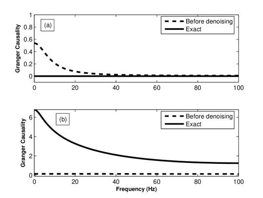
Figure 1: Granger causality spectra for a bivariate AR(1) process (a) Causality of $X\rightarrow Y$ (b) Causality of $Y\rightarrow X$. The solid lines represent true causality spectra and the dashed lines represent spectra from noisy data.

We now estimate the Granger causality spectrum for the specific AR(1) process given in Eq. (21) where $Y$ drives $X$ and $X$ does not drive $Y$. The parameter values used are $a=0.4$, $b=0.6$, $d=0.9$, $\sigma_{\xi}=0.2$ and $\sigma_{\eta}=1.0$. We obtain two time series $X$ and $Y$ by numerically simulating the VAR model and then adding Gaussian measurement noise with $\sigma_{\xi^{\prime}}=0.2$ and $\sigma_{\eta^{\prime}}=2.5$. For concreteness we assume that each time unit corresponds to 5 ms. In other words, the sampling rate is 200 Hz, and thus the Nyquist frequency is 100 Hz. The dataset consists of one hundred realizations, each of length 250 ms (50 points). These 100 realizations are used to obtain expected values of the covariance matrices in the LWR and KEM algorithms (see next section). The Granger causality spectra $I_{X\rightarrow Y}(f)$ and $I_{Y\rightarrow X}(f)$ are plotted in Figure 1. The solid lines represents the true causality spectra while the dashed lines represent the noisy causality spectra.

Similarly, we also simulated the following bivariate AR(2) process:

$${X(t)} = a{X(t-1)}+b{Y(t-1)}+E_{1}(t),$$

$${Y(t)} = d_{1}{Y(t-1)}+d_{2}{Y(t-2)}+E_{2}(t).$$ (35)

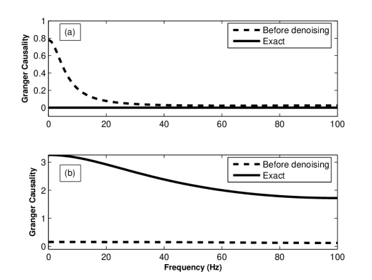
Figure 2: Granger causality spectra for a bivariate AR(2) process (a) Causality of $X\rightarrow Y$ (b) Causality of $Y\rightarrow X$. The solid lines represent true causality spectra and the dashed lines represent spectra from noisy data.

The values of the parameters $a$ and $b$ used were the same as in the previous AR(1) process example (Eq. 21) except for the values of the new parameters $d_{1}$ and $d_{2}$ which were chosen to be 0.4 and 0.5 respectively. We again obtain two time series $X$ and $Y$ and then added Gaussian measurement noise with $\sigma_{\xi^{\prime}}=0.2$ and $\sigma_{\eta^{\prime}}=2.5$ to $X$ and $Y$ respectively. The Granger causality spectra $I_{X\rightarrow Y}(f)$ and $I_{Y\rightarrow X}(f)$ are plotted in Figure 2. As before, the solid lines and dashed lines represent the true causality spectra and noisy causality spectra, respectively.

We observe that the measurement noise has a dramatic effect in both of these cases: It completely reverses the true causal directions. For the noisy data, $X$ appears to drive $Y$ and $Y$ does not appear to drive $X$.

The above theoretical and numerical results bring out clearly the adverse effect that noise can have on correctly determining directional influences. The same is also true for other quantities like power spectrum and coherence. Therefore it is imperative that the effect of noise be mitigated to the extent possible.

IV The KEM Denoising Algorithm

In the previous section we have seen that noisy data can lead to grave misinterpretation of directional influences. We now provide a practical solution to this problem by combining the Kalman smoother with the Expectation-Maximization algorithm EM . The detailed algorithm is long and tedious. We outline the main logical steps below.

Kalman filter Kalman is a standard algorithm for denoising noisy data. To apply this, we first need to recast a VAR process with measurement noise in the so-called state-space form. This is nothing but the difference equation analogue of converting a higher order differential equation to a system of first order differential equations. Once this is done, our VAR model takes on the following form:

$$\mathbf{x}_{t+1} = A\mathbf{x}_{t}+\mathbf{w}_{t+1},$$ (36)

$$\mathbf{y}_{t} = C\mathbf{x}_{t}+\mathbf{v}_{t}.$$ (37)

Here $\mathbf{x}_{t}$ is an $M\times 1$ (“true”) state vector at time $t$. $A$ is an $M\times M$ state matrix. $\mathbf{w}_{t}$ is a zero mean Gaussian independent and identically distributed random variable with covariance matrix $Q$. Bivariate AR(p) models can be put in the form $\mathbf{x}_{t+1}=A\mathbf{x}_{t}+\mathbf{w}_{t+1}$ by defining $M=2p$ auxiliary variables $x_{i,t}$. The $N\times 1$ vector $\mathbf{y}_{t}$ is the observed/measured value of $\mathbf{x}_{t}$ in $N$ channels. $C$ is an $N\times M$ observation matrix and is a fixed, known matrix for VAR models. Hence we will ignore this in future discussions. The $N\times 1$ vector $\mathbf{v}_{t}$ is the measurement noise which is zero mean, Gaussian, independent and identically distributed with covariance matrix $R$.

Kalman filter, however, can not be directly applied to denoise experimental or observed data since it assumes the knowledge of the model describing the state space dynamics. In practice, such knowledge is often not available. To get around this problem, we apply the Kalman smoother in conjunction with the Expectation and Maximization algorithm EM ; Gahramani ; Weinstein ; Digalakis . Thus, this denoising algorithm will henceforth be called the KEM algorithm. In this algorithm, one follows the standard procedure for estimating state space parameters from data using the maximum likelihood method. The appropriate likelihood function in our case is the joint log likelihood log$P(\{\mathbf{x}\},\{\mathbf{y}\})$ where $\{\mathbf{x}\}$ denotes $\{\mathbf{x}_{t}\}$ (for all $t$) and similarly for $\{\mathbf{y}\}$. In the usual maximum likelihood method, $P$ would not depend on ${\mathbf{x}}$ and we would therefore maximize the above quantity directly (conditioned on the observed $\mathbf{y}_{t}$ values) and obtain the unknown state space parameters. But in our case, $P$ depends on $\mathbf{x}$ which is also unknown. To get rid of $\mathbf{x}$, we take the expected value of the log likelihood

$$O=E[\log P(\{\mathbf{x}\},\{\mathbf{y}\})\mid\{\mathbf{y}\}].$$

As usual, we have conditioned the expectation on the known observations $\{\mathbf{y}\}$.

To compute $O$, it turns out we need the expectations of $\mathbf{x}$ and $\mathbf{x}\mathbf{x}^{T}$ (where $T$ denotes the transpose) conditioned on $\mathbf{y}$. These expectations are obtained by applying the Kalman smoother on the noisy data. We use the Kalman smoother and not the Kalman filter since we are utilizing all the observations $\mathbf{y}$ instead of only the past observations. This is the appropriate thing to do in our case since we are performing an off-line analysis where all observations are known. In other words, in Kalman smoother, we perform both a forward pass and a backward pass on the data in order to make use of all observations.

To apply the Kalman smoother, however, we still need the state space model parameters (just as in the Kalman filter case). To circumvent this problem, we start with initial estimates for these parameters ($A$, $Q$ and $R$) as follows. From the noisy data, using the LWR algorithm, we obtain the VAR model coefficient matrices Ding . Then a standard transformation Kalman is used to put these matrices in the state space form giving the initial estimate for $A$. The initial estimate of $Q$ is taken to be the identity matrix following the standard procedure Kalman . The initial estimate of $R$ is taken to be half the covariance matrix at lag zero of the noisy data. The approximate model order can be determined by applying the AIC criterion akaike in the LWR algorithm. This step is admittedly rather ad hoc. Further studies to optimize the above initial estimates and the VAR model order $p$ are currently being carried out. Once we have initial estimates of the model parameters, we can apply the Kalman smoother to obtain the various conditional expectations and evaluate the expected log likelihood $O$. This is called the expectation (E) step.

Next, we go to the maximization (M) step. Each of the parameters $A,Q,R$ etc is re-estimated by maximizing $O$. Using these improved estimates, we can apply the E step again followed by the M step. This iterative process is continued till the value of log likelihood function converges to a maximum. We could now directly use the VAR parameters estimated from the KEM algorithm for further analysis as is usually done. But here we prefer to use the following procedure which was found to yield better performance. The final denoised data (that is, the estimate of $\mathbf{x}$ obtained from the KEM algorithm) is treated as the new experimental time series and subjected to parametric spectral analysis from which Granger causality measures can be derived. The Matlab code implementing this algorithm for our applications is available from the authors upon request.

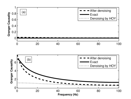
Figure 3: Granger causality spectra for the bivariate AR(1) process in Fig 1. (a) Causality of $X\rightarrow Y$ (b) Causality of $Y\rightarrow X$. The solid lines represent true causality spectra and the dashed lines represent spectra obtained from the denoised data using the KEM algorithm. The dotted lines represent spectra obtained using HOY algorithm.

We have compared the denoising capabilities of the KEM algorithm with two widely used algorithms, the higher-order Yule-Walker (HOY) method Chan and the overdetermined higher-order Yule-Walker method Cadzow . We find that the denoising capabilities of the KEM algorithm is superior. Detailed results will be presented elsewhere. In Figure 3, we explicitly show that KEM algorithm performs better than the HOY method (see below).

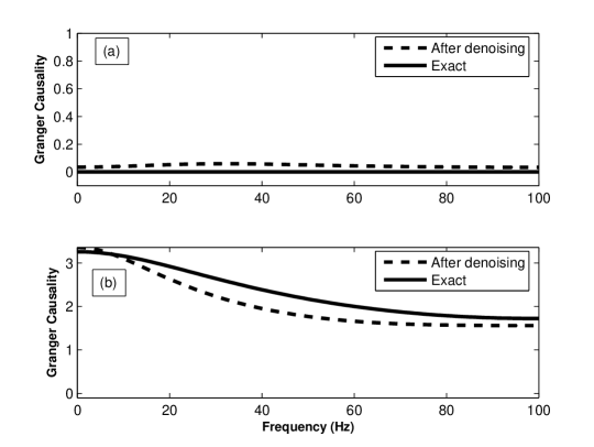
Figure 4: Granger causality spectra for the bivariate AR(2) process in Fig 2. (a) Causality of $X\rightarrow Y$ (b) Causality of $Y\rightarrow X$. The solid lines represent true causality spectra and the dashed lines represent spectra obtained from the denoised data using the KEM algorithm.

The KEM algorithm is applied to denoise the data shown in Figures 1 and 2. Figure 3 displays the same exact Granger causality spectra (solid lines) as that in Figure 1 and the Granger causality spectra (dashed lines) obtained from the denoised data using KEM algorithm. Causality spectra obtained using HOY method is also shown (as dotted lines). It is clear that the KEM method performs better. In Figure 4, the solid lines again represent the same exact Granger causality as that in Figure 2 and the dashed lines represent the Granger causality spectra obtained from the denoised data of a bivariate AR(2) process. We see that the correct causal directions are recovered and that the denoised spectra are reasonably close to the true causality spectra for both AR(1) and AR(2) process. We stress that these results are achieved without assuming any knowledge of the VAR models [Eqs. 21 and 35] that generated the original time series data.

V Causal relations in a neural network model

In this section, we analyze the effect of noise on time series generated by a neural network model. We first demonstrate the effect of measurement noise on causality directions and then the effect of applying the KEM algorithm on the noisy data.

Our simulation model comprises two coupled cortical columns where each column is made up of an excitatory and an inhibitory neuronal population kaminski_2001 . The equations governing the dynamics of the two columns are given by

$$\ddot{x_{i}}+(a+b)\dot{x_{i}}+abx_{i} = -k_{ei}Q(y_{i}(t),Q_{m0})+k_{ij}Q(x_{j}(t),Q_{m0})+\xi_{x_{i}}(t),$$ (38)

$$\ddot{y_{i}}+(a+b)\dot{y_{i}}+aby_{i} = k_{ie}Q(x_{i}(t),Q_{m0})+\xi_{y_{i}}(t),$$ (39)

where $i\neq j=1,2$. Here $x$ and $y$ represent local field potentials (LFP) of the excitatory and inhibitory populations respectively, $k_{ie}>0$ gives the coupling gain from the excitatory $(x)$ to the inhibitory $(y)$ population, and $k_{ei}>0$ is the strength of the reciprocal coupling. The neuronal populations are coupled through a sigmoidal function $Q(x,Q_{m0})$ which represents the pulse densities converted from $x$ with $Q_{m0}$ a modulatory parameter. The function $Q(x,Q_{m0})$ is defined by

$$Q(x,Q_{m0})=\left\{\begin{array}[]{ll}Q_{m0}[1-e^{-(e^{x}-1)/Q_{m0}}]&\mbox{if $x>-u_{0}$ }\\ -1&\mbox{if $x\leq-u_{0}$}\end{array}\right.,$$ (40)

where $u_{0}=-\ln[1+\ln(1+\frac{1}{Q_{m0}})].$ The coupling strength $k_{ij}$ is the gain from the excitatory population of column $j$ to the excitatory population of column $i$, with $k_{ij}=0$ for $i=j.$ The terms $\xi(t)$ represent independent Gaussian white noise inputs given to each neuronal population.

The parameter values used were: $a=0.22/$ms, $b=0.72/$ms, $k_{ie}=0.1,k_{ei}=0.4,k_{12}=0,k_{21}=0.25$ and $Q_{m0}=5$. The standard deviation for the Gaussian white noise was chosen as 0.2. Assuming a sampling rate of 200Hz, two hundred realizations of the signals were generated, each of length 30 s (6,000 points).

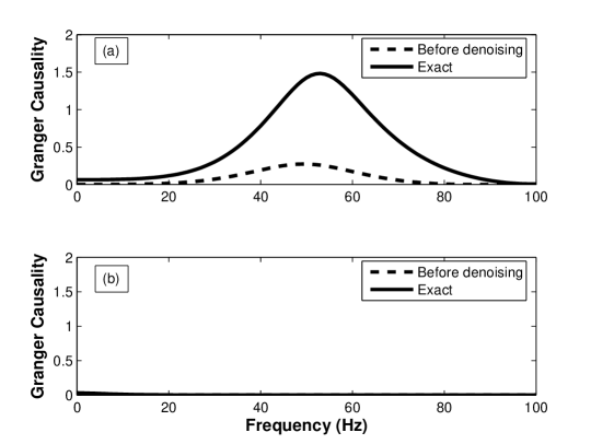
Figure 5: Granger causality spectra for noisy data from a neural network model (a) Causality of $x_{1}\rightarrow x_{2}$ (b) Causality of $x_{2}\rightarrow x_{1}$. The solid lines represent true causality spectra (noise-free data) and the dashed lines represent spectra from noisy data.

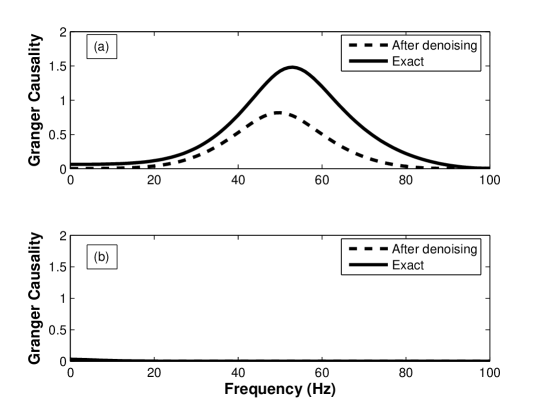
Figure 6: Granger causality spectra of the neural network model (a) Causality of $x_{1}\rightarrow x_{2}$ (b) Causality of $x_{2}\rightarrow x_{1}$. The solid lines represent true causality spectra (noise-free data) and the dashed lines represent spectra obtained from denoised data using the KEM algorithm.

We now restrict our attention to the variables $x_{1}(t)$ and $x_{2}(t)$. Measurement noises (Gaussian white noises with standard deviations 2.0 and 3.0 respectively) were added to these variables. From the model it is clear that $x_{1}(t)$ should drive $x_{2}(t)$ since $k_{12}=0$ while $k_{21}=0.25$. The results of applying Granger causality analysis (using a VAR model of order 7) on these two variables is shown in Figure 5. The solid lines represent the causality spectra for the noise-free data. The dashed lines represents the causality spectra for the noisy data. It is clear that the measurement noise has an effect on the causal relations by significantly reducing the true causality magnitude. In contrast to the example in Section 3, however, no spurious causal direction is generated here, despite the fact that both time series are contaminated by measurement noise. Next, we applied the KEM algorithm to denoise the noisy data. When Granger causality analysis is performed on the denoised data, we obtain causality spectra that are closer to the true causality spectra (see Figure 6). We note that the KEM algorithm is not able to completely remove the noise as the denoised spectra are still quite different from the true spectra.

To show that the denoised Granger spectrum is significantly different from that of the noisy data we use the bootstrap approach efron to establish the significant difference between the two peaks observed in Granger causality spectrum of Figures 5 and 6 (shown by dashed lines in these Figures). One thousand resamples of noisy data and the denoised data were generated by randomly selecting trials with replacement. It should be noted that in any selected trial, the entire multichannel data is taken as it is thus preserving the auto and cross correlation structures. Thus, we employ a version of block bootstrap method efron . The peak values of Granger causality were computed for each resample using both noisy data and denoised data. Let us denote these peak values by the random variables $Z_{1}$ and $Z_{2}$ respectively. The two population Student t-test was performed to determine whether the means of $Z_{1}$ and $Z_{2}$ are different at a statistically significant level.

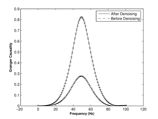
Figure 7: Granger causality spectra of the neural network model for the direction $x_{1}\rightarrow x_{2}$. The solid line represents the Granger causality for denoised data, while the dashed line represents the Granger causality for noisy data. 95% confidence intervals are also given..

The null hypothesis was that the means of the two populations $Z_{1}$ and $Z_{2}$ are equal. The $t$ value was found to be very large: $4.6446*10^{3}$ and corresponds to a two-tailed $p$ value less than 0.0001. Thus the null hypothesis that the two groups do not differ in mean is rejected. This establishes the fact that the peak of the Granger causality spectrum of the denoised data is significantly higher than that of the noisy data. Figure 7 shows the plot of Granger causality for the direction $x_{1}\rightarrow x_{2}$ along with 95% confidence intervals. The 95% confidence intervals are calculated as $I_{x_{1}\rightarrow x_{2}}(f)\pm 1.96\sigma_{B}$ (for each frequency $f$) where $\sigma_{B}$ is the sample standard deviation of the $1000$ bootstrap replications of $I_{x_{1}\rightarrow x_{2}}(f)$.

VI Conclusions

Our contributions in this paper are two fold. First, we demonstrate that measurement noise can significantly impact Granger causality analysis. Based on analytical expressions linking noise strengths and the VAR model parameters, it was shown that spurious causality can arise and that true causality can be suppressed due to noise contamination. Numerical simulations were performed to illustrate the theoretical results. Second, a practical solution to the measurement noise problem, called the KEM algorithm, was outlined, which combines the Kalman filter theory with the Expectation and Maximization (EM) algorithm. It was shown that the application of this algorithm to denoise the noisy data can significantly mitigate the deleterious effects of measurement noise on Granger causality estimation. It is worth noting that, despite the fact that the adverse effect of measurement noise on Granger causality has been known since 1978 Newbold , mitigation of such effect has received little attention. The KEM algorithm described in this paper is our attempt at addressing this shortcoming.

Appendix

In this appendix, we derive the expressions for $P_{3}(B)$ and $P_{4}(B)$ given in Eq. (22). We first determine $P_{4}(B)$. When a zero mean white noise process $\eta^{\prime}(t)$ with variance $\sigma_{\eta^{\prime}}^{2}$ is added to $Y(t)$ we get

$${Y^{(c)}(t)}={Y(t)+\eta^{\prime}(t)}.$$ (41)

Applying $(1-dB)$ on both sides of the above equation we get

$$(1-dB){Y^{(c)}(t)} = (1-dB){Y(t)}+(1-dB){\eta^{\prime}(t)}$$ (42)

$$= {\eta(t)}+(1-dB){\eta^{\prime}(t)}.$$

We now determine a white noise process ${\eta^{(c)}(t)}$ such that

$${\eta(t)}+(1-dB){\eta^{\prime}(t)}=(1-d^{\prime}B){\eta^{(c)}(t)}.$$ (43)

We need to determine $d^{\prime}$ and ${\sigma_{\eta^{(c)}}^{2}}$.

Taking variances on both sides of the above equation we get

$${\sigma_{\eta}^{2}}+(1+d^{2}){\sigma_{\eta^{\prime}}^{2}}=(1+d^{\prime 2}){\sigma_{\eta^{(c)}}^{2}}.$$ (44)

Taking autocovariance at lag 1 on both sides we obtain

$$d{\sigma_{\eta^{\prime}}^{2}}=d^{\prime}{\sigma_{\eta^{(c)}}^{2}}.$$ (45)

Since ${\eta^{(c)}}$ is a sum of ${\eta}$ and $(1-dB){\eta^{\prime}}$, we have ${\sigma_{\eta^{(c)}}^{2}}>{{\sigma_{\eta^{\prime}}^{2}}}.$ This implies that $|d^{\prime}|<|d|$. Since stationarity of the AR process requires $0<|d|<1$, we obtain the inequality $0<|d^{\prime}|<|d^{\prime}|<1.$ Further $d^{\prime}$ has the same sign as $d$.

We have

$${\sigma_{\eta^{(c)}}^{2}}=\frac{d}{d^{\prime}}{\sigma_{\eta^{\prime}}^{2}}.$$ (46)

Substituting in the variance equation we get

$$(1+d~{}^{{{}^{\prime}}{2}})\frac{d}{d^{\prime}}{\sigma_{\eta^{\prime}}^{2}}=(1+d^{2}){\sigma_{\eta^{\prime}}^{2}}+{\sigma_{\eta}^{2}},$$ (47)

that is,

$$(\frac{1}{d^{\prime}}+d^{\prime})=(\frac{1}{d}+d)+\frac{1}{d}\frac{{\sigma_{\eta}^{2}}}{{\sigma_{\eta^{\prime}}^{2}}}.$$ (48)

Let

$$s\equiv(\frac{1}{d}+d)+\frac{1}{d}\frac{{\sigma_{\eta}^{2}}}{{\sigma_{\eta^{\prime}}^{2}}}.$$

This gives

$$(\frac{1}{d^{\prime}}+d^{\prime})=s.$$ (49)

Hence

$$d^{\prime}=\frac{s{\pm{\sqrt{s^{2}-{4}}}}}{2}.$$ (50)

Note that $|s|>2$ for any value of $d$, ${\sigma_{\eta}^{2}}$, and ${\sigma_{\eta^{\prime}}^{2}}$. Therefore $\sqrt{s^{2}-{4}}$ and hence $d{{}^{\prime}}$ are well defined. Further, since $|d{{}^{\prime}}|<|d|$ if $d$ is positive, $d^{\prime}=({s-\sqrt{s^{2}-{4}}})/{2}$ is the only valid solution. If $d$ is negative, $d^{\prime}=({s+\sqrt{s^{2}-{4}}})/{2}$ is the only valid solution.

Next, we derive the expression for $P_{3}(B)$. First, we first need to rewrite ${X(t)}$ as an univariate process i.e. we need to determine $P_{1}(B)$:

$$P_{1}(B)X(t)=\xi(t),$$ (51)

where $\xi(t)$ is a zero mean white noise process and

$${X(t)}=a{X(t-1)}+b{Y(t-1)}+E_{1}(t).$$ (52)

Here $E_{1}(t)$ is a zero mean white noise process with variance $\sigma_{\epsilon}^{2}$. We have already seen that

$$(1-dB){Y(t)}={\eta(t)}.$$ (53)

The equation for $X(t)$ can be written as

$$(1-aB){X(t)}=b{Y(t-1)}+E_{1}(t).$$ (54)

Substituting the expression for $Y(t-1)$ we obtain

$$(1-aB){X(t)}=b(1-dB)^{-1}{\eta(t-1)}+E_{1}(t).$$ (55)

We now find a white noise process ${\xi(t)}$ with variance ${\sigma_{\xi}^{2}}$ such that

$$b(1-dB)^{-1}{\eta(t-1)}+E_{1}(t)=(1-rB)^{-1}{\xi(t)}.$$ (56)

To determine ${r}$ and ${\sigma_{\xi}^{2}}$, we take variance and autocovariance at lag 1 on both sides. Taking variance we obtain

$$\frac{b^{2}{\sigma_{\eta}^{2}}}{(1-d^{2})}+{\sigma_{\epsilon}^{2}}=\frac{{\sigma_{\xi}^{2}}}{(1-r^{2})}.$$ (57)

Taking autocovariance at lag 1 and assuming that $\sigma_{\epsilon\eta}$ (the cross-covariance between $E_{1}$ and $\xi$) is zero for simplicity, we get

$$\frac{b^{2}\sigma_{\eta}^{2}d}{(1-d^{2})}=\frac{{\sigma_{\xi}^{2}}}{(1-r^{2})},$$ (58)

which can be written as

$$\frac{{\sigma_{\xi}^{2}}}{(1-r^{2})}=\frac{b^{2}{\sigma_{\eta}^{2}}{d}}{(1-d^{2})r}.$$ (59)

Substituting in the variance equation we obtain

$$\frac{b^{2}{\sigma_{\eta}^{2}}}{(1-d^{2})}+{\sigma_{\epsilon}^{2}}=\frac{b^{2}{\sigma_{\eta}^{2}}}{(1-d^{2})}\frac{d}{r}.$$ (60)

Thus

$$r=\frac{b^{2}d{\sigma_{\eta}^{2}}}{b^{2}{\sigma_{\eta}^{2}}+(1-d^{2}){\sigma_{1}^{2}}}.$$ (61)

If $b=0$, we get $r=0$ and ${\sigma_{\xi}^{2}}={\sigma_{1}^{2}}$ as expected. Similarly if $d=0$, we get $r=0$ and ${\sigma_{\xi}^{2}}={\sigma_{1}^{2}}+b^{2}{\sigma_{\eta}^{2}}$ as expected. Once $r$ is known, ${\sigma_{\xi}^{2}}$ is given by

$${\sigma_{\xi}^{2}}=(1-r^{2})\left[\frac{b^{2}{\sigma_{\eta}^{2}}}{(1-d^{2})}+{\sigma_{1}^{2}}\right].$$ (62)

We finally have

$$(1-aB){X(t)}=(1-rB)^{-1}{\xi(t)}.$$ (63)

That is,

$$P_{1}(B)X(t)=\xi(t),\ \ \ P_{1}{(B)}=(1-rB)(1-aB).$$ (64)

Consider a white noise process $\xi^{\prime}(t)$ (which is uncorrelated with $X(t)$) and has variance $\sigma_{\xi^{\prime}}^{2}$. This is added to $X(t)$ to obtain the noisy process $X^{(c)}(t)$:

$$X^{(c)}(t)=X(t)+\xi^{\prime}{(t)}.$$ (65)

Applying $P_{1}(B)$ on both sides of the above equation,

$$P_{1}(B)X^{(c)}(t)=\xi(t)+P_{1}{(B)}\xi^{\prime}{(t)}.$$ (66)

We need to find a zero mean white noise process $\xi^{(c)}{(t)}$ with variance $\sigma_{\xi^{(c)}}^{2}$ such that

$$\xi(t)+P_{1}{(B)}\xi^{\prime}{(t)}=P_{3}{(B)}\xi^{(c)}{(t)}.$$ (67)

Let

$$P_{3}(B)=1+a_{1}^{{}^{\prime}}B+a_{2}^{{}^{\prime}}B^{2}.$$ (68)

We have

$$\xi(t)+(1-(a+r)B+arB^{2})\xi^{\prime}(t)=[1+a_{1}^{{}^{\prime}}B+a_{2}^{{}^{\prime}}B^{2}]\xi^{(c)}(t).$$ (69)

Taking variances on both sides we get

$$\sigma_{\xi}^{2}+(1+(a+r)^{2}+a^{2}r^{2})\sigma_{\xi^{\prime}}^{2}=[1+a_{1}^{\prime{\ 2}}+a_{2}^{\prime{\ 2}}]\sigma_{\xi^{(c)}}^{2}.$$ (70)

Taking autocovariance at lag 1 on both sides we obtain

$$-(a+r)\sigma_{\xi^{\prime}}^{2}-ar(a+r)\sigma_{\xi^{\prime}}^{2}=a_{1}^{{}^{\prime}}\sigma_{\xi^{(c)}}^{2}+a_{1}^{{}^{\prime}}a_{2}^{{}^{\prime}}\sigma_{\xi^{(c)}}^{2}.$$ (71)

This can be rewritten as

$$-(a+r)(1+ar)\sigma_{\xi^{\prime}}^{2}=a_{1}^{{}^{\prime}}(1+a_{2}^{{}^{\prime}})\sigma_{\xi^{(c)}}^{2}.$$ (72)

Taking autocovariance at lag 2 on both sides

$$ar\sigma_{\xi^{\prime}}^{2}=a_{2}^{{}^{\prime}}\sigma_{\xi^{(c)}}^{2},$$ (73)

which gives

$$\sigma_{\xi^{(c)}}^{2}=\frac{ar}{a_{2}^{{}^{\prime}}}\sigma_{\xi^{\prime}}^{2}.$$ (74)

Since $\sigma_{\xi^{(c)}}^{2}>\sigma_{\xi^{\prime}}^{2}$, we see that $|a_{2}^{{}^{\prime}}|<|ar|$ and $a_{2}^{\,{}^{\prime}}$ has the same sign as $ar$.

Substituting the last equation in Eqs. (72) and (70) we obtain

$$-(a+r)(1+ar)\sigma_{\xi^{\prime}}^{2}=a_{1}^{{}^{\prime}}(1+a_{2}^{{}^{\prime}})\frac{ar}{a_{2}^{{}^{\prime}}}\sigma_{\xi^{\prime}}^{2},$$ (75)

and

$$\sigma_{\xi}^{2}+[1+(a+r)^{2}+a^{2}r^{2}]\sigma_{\xi^{\prime}}^{2}=[1+a_{1}^{\prime{2}}+a_{2}^{\prime{2}}]\frac{ar}{a_{2}^{{}^{\prime}}}\sigma_{\xi^{\prime}}^{2}.$$ (76)

Thus we get

$$\frac{a_{1}^{{}^{\prime}}(1+{a_{2}^{{}^{\prime}})}}{a_{2}^{{}^{\prime}}}=-\frac{(a+r)(1+ar)}{ar},$$ (77)

and

$$\frac{(1+a_{1}^{\prime{2}}+a_{2}^{\prime{2}})}{a_{2}^{\prime}}=\frac{[1+(a+r)^{2}+a^{2}r^{2}]}{a_{r}}+\frac{1}{ar}\frac{{\sigma_{\xi}^{2}}}{{\sigma_{\xi^{\prime}}^{2}}}.$$ (78)

We can solve these two equations for $a_{1}^{{}^{\prime}}$ and $a_{2}^{{}^{\prime}}$. There will be multiple solutions. We choose that solution for which $|a_{2}^{{}^{\prime}}|<|ar|$. Further the solution has to be such that the roots of $1+a_{1}^{{}^{\prime}}B+a_{2}^{{}^{\prime}}B^{2}=0$ lie outside the unit circle. The last condition is required for the invertibility of the MA process $(1+a_{1}^{{}^{\prime}}B+a_{2}^{{}^{\prime}}B^{2})\xi^{(c)}(t)$. The expressions for $a_{1}^{{}^{\prime}}$ and $a_{2}^{{}^{\prime}}$ obtained by solving the above equations are very long and therefore we do not list them here. However, we can easily obtain the asymptotic behaviour of these solutions as follows.

For our bivariate AR(1)process to be stable, we require that the roots of

$$\det[\lambda I-A(1)]=0$$ (79)

lie within the unit circle i.e., the eigenvalues of A(1) should have absolute value less than 1. In our case

$${A(1)}={\left(\begin{array}[]{cc}a&b\\ 0&d\end{array}\right)},$$

which is an upper triangular matrix. Hence eigenvalues are $a$ and $d$. Therefore, for stability we require that $|a|<1$ and $|d|<1$.

As already derived, we have

$$r=d{\left(\frac{b^{2}{\sigma_{\eta}^{2}}}{b^{2}{\sigma_{\eta}^{2}}+(1-d^{2}){\sigma_{\xi}^{2}}}\right)}.$$ (80)

Since $|d|<1$, the term within brackets is always positive and less than 1. It becomes zero only when $b=0$. Hence $|r|<|d|$ and $r$ has same sign as $d$. As $|d|\rightarrow 1$, $|r|\rightarrow 1$. As $|d|\rightarrow 0$ or $|b|\rightarrow 0$, we see that $|r|\rightarrow 0$.

We have already seen that $|a_{2}^{{}^{\prime}}|<|ar|$. Since $|r|<|d|$, we obtain further results that $|a_{2}^{{}^{\prime}}|<|a||d|$ and $a_{2}^{{}^{\prime}}$ has same sign as $ad$. Since $|a|,|d|<1$, we get

$$0<|a_{2}^{\,{}^{\prime}}|<|a||d|<1.$$

As $|a|,|d|\rightarrow 1$, $|a_{2}^{{}^{\prime}}|~{}\rm{also}~{}\rightarrow 1$. As $a\rightarrow 1$, $d\rightarrow 1$ and the ratio ${\sigma_{\xi}^{2}}/{\sigma_{\xi^{\prime}}^{2}}\rightarrow 0$, we have

$$a_{1}^{\,{}^{\prime}}\rightarrow{-2};a_{1}^{{}^{\prime}}\rightarrow 1.$$

As the variance ratio $\rightarrow\infty$

$$a_{1}^{{}^{\prime}}\rightarrow 0;a_{2}^{\,{}^{\prime}}\rightarrow 0,$$

as expected. The parameter $a_{1}^{\,{}^{\prime}}$ is hardly affected by the value of the parameter $b$. On the other hand, $a_{2}^{\,{}^{\prime}}\rightarrow 0$ as $b\rightarrow 0$ and saturates rapidly for $b>0.5$.

References

- (1) C. W. J. Granger, Econometrica 37, 424 (1969).
- (2) K. J. Blinowska, R. Kus and M. Kaminski, Phys. Rev. E 70, 050902 (2004).
- (3) D. Marinazzo, M. Pellicoro and S. Stramaglia, Phys. Rev. E 73 066216 (2006).
- (4) P. F. Verdes, Phys. Rev. E 72, 026222 (2005).
- (5) N. G. Rosenblum and A. S. Pikovsky, Phys. Rev. E 64 045202 (2001).
- (6) X. Hu and V. Nenov, Phys. Rev. E 69 026206 (2004).
- (7) L. M. Xu, Z. Chen, K. Hu, H. E. Stanley and P. Ch. Ivanov, Phys. Rev. E 73 065201 (2006).
- (8) M. Ding, S. L. Bressler, W. Yang, and H. Liang, Biol. Cyber. 84, 463 (2000).
- (9) A. Brovelli, M. Ding, A. Ledberg, Y. Chen, R. Nakamura, and S. L. Bressler, Proc. Natl. Acad. Sci. USA 101, 9849 (2004).
- (10) D. L. Thornton and D. S. Batten, Journal of Money, Credit and Banking 17, 164 (1985).
- (11) T. E. Hall and N. R. Noble, Journal of Money, Credit and Banking 19, 112 (1987).
- (12) C. Hiemstra and J. D. Jones, Journal of Finance 49, 1639 (1994).
- (13) Y. Chen, G. Rangarajan, J. Feng, and M. Ding, Physics Letters A 324, 26 (2004).
- (14) R. Ganapathy, G. Rangarajan, and A. K. Sood, Phys. Rev. E 75, 016211 (2007).
- (15) W. A. Fuller, Measurement Error Models, (John Wiley and Sons, New York, 1987).
- (16) P. Newbold, Int. Econ. Rev. 19, 787 (1978).
- (17) D. A. Pierce and L. D. Haugh, J. Econometrics 5, 265 (1977).
- (18) C. W. J. Granger and M. J. Morris, J. Royal Statist. Soc. Ser. A 139, 246 (1976).
- (19) A. Maravall and A. Mathis, J. Econometrics 61, 197 (1994).
- (20) C. Chatfield, The Analysis of Time Series, (Chapman and Hall, Boca Raton, 2004).
- (21) M. Morf, A. Vieira, D. Lee, and T. Kailath, IEEE Trans Geoscience Electronics 16, 85 (1978).
- (22) J. Geweke, J. Amer. Statist. Assoc. 77, 304 (1982).
- (23) Y. Hosoya, Prob. Th. Related Fields 88, 429 (1991).
- (24) A. P. Dempster, N. M. Laird, and D. B. Rubin, J. Royal Statist. Soc. Ser. B 39, 1 (1977).
- (25) S. Haykin, Adaptive Filter Theory (Prentice-Hall, New York, 2001).
- (26) Z. Gahramani and G. E. Hinton, Technical Report CRG-TR-96-2, 1996.
- (27) E. Weinstein, A. V. Oppenheim, M. Feder, and J. R. Buck, IEEE Trans Signal Proc. 42, 846 (1994).
- (28) V. Digalakis, J. R. Rohlicek, and M. Ostendorf, IEEE Trans Speech Audio Proc. 1, 431 (1993).
- (29) H. Akaike, IEEE Trans Autom Control AC-19, 716 (1974).
- (30) Y. T. Chan and R. Langford, IEEE Trans. Acoustics, Speech and Signal Proc. 30, 689 (1980).
- (31) J. A. Cadzow, Proc. IEEE 70, 907 (1982).
- (32) M. Kaminski, M. Ding, W. A. Truccolo, and S. L. Bressler, Biol. Cybern. 85, 145 (2001).
- (33) B. Efron, The Jackknife,the Bootstrap, and Other Repsampling Plans (SIAM, Philadephia, 1982).