Generating Function in Quantum Mechanics: An Application to Counting Problems

Abstract

In this paper we present a generating function approach to two counting problems in elementary quantum mechanics. The first is to find the total ways of distributing $N$ identical particles among $m$ different states. The second is to find the degeneracies of energy levels in a quantum system with multiple degrees of freedom. Our approach provides an alternative to the methods in textbooks.

I Introduction

Generating function (GF) is a terminology frequently used in combinatorial mathematics as a bridge between discrete mathematics and continuous analysis. It functions like a clothesline on which we hang up a sequence of numbers for display Wilf . A GF may have different aliases in different contexts, e.g. partition function in statistical physics Huang and $Z$-transform in signal analysis Oppenheim . It can be used to find certain characteristics of a sequence like expectation value or standard deviation Papoulis . Sometimes that will be much more efficient than a direct evaluation.

There are many ways to construct a GF for a sequence, the simplest of which is using power series. Given $\{a_{n}\}$ ($n\geq 0$), we may construct its GF as

$$F(t)=\sum_{n\geq 0}a_{n}t^{n}.$$ (1)

Note that $t$ can take a continous value and $F(t)$ is analytic with respect to $t$, which may give us some computational power using techniques of derivation or integration.

The paper is organized as follows. Section II shows how a GF can find the number of distinct ways of assigning $N$ identical bosons or fermions to $m$ different states. Section III discusses the GF approach to find the degeneracies of energy levels of a harmonic oscillator and a confined free particle both in higher dimensions. In our discussion, we follow the notation $[t^{n}]\,F(t)$ used in Ref. Wilf to mean the coefficient of $t^{n}$ term in the power series expansion of $F(t)$. For example, we have $[t^{n}]\,\mathrm{e}^{t}=1/{n!}$ $(n\geq 0)$.

II finding total ways of distributing identical particles

The problem of how many ways there are to distribute $N$ identical particles among $m$ different states lies at the heart of quantum statistics. It determines the specific distribution function that identical particles obey, i.e. Bose-Einstein distribution for bosons and Fermi-Dirac distribution for fermions. Textbooks generally tackle the problem by a combinatorial method Griffiths . Here we show how to solve it by a GF.

II.1 Identical Fermions

Pauli’s exclusion principle has that a quantum state can accommodate one fermion at most. This makes the counting problem to be much easier than that of bosons. The number is simply the binomial coefficient $m$ choose $N$:

$${m\choose N}=\frac{m!}{N!\,(m-N)!}.$$ (2)

We can do it in another way. The occupation number for fermions is $0$ and $1$ only. We thus associate each state with a GF $F(t)=t^{0}+t^{1}=1+t$. It is obvious that the coefficient of term $t^{N}$ in the expansion of $F^{m}(t)$ is exactly the total ways that we can pick out $N$ candidates from $m$ states: ($N\leq m$)

$${[t^{N}]}F^{m}(t) = {[t^{N}]}\,(1+t)^{m}$$ (3)

$$= \frac{1}{N!}\,{[t^{0}]}\,\frac{\mathrm{d}^{N}}{\mathrm{d}x^{N}}\,(1+t)^{m}$$

$$= \frac{1}{N!}\,{[t^{0}]}\,m(m-1)\cdots(m-N+1)(1+t)^{m-N}$$

$$= \frac{m!}{N!\,(m-N)!}$$

$$= {m\choose N}.$$

The GF approach recovers the binomial coefficient $m$ choose $N$. Furthermore, the approach can be easily adapted to the boson case.

II.2 Identical Bosons

There can be an arbitrary number of bosons in one quantum state in principle, i.e. the occupation number can be $0$,$1$,$2$,$\cdots$. It is not easy to figure out a combinatorial method to find the total ways in this case. With the help of GF, we now associate each quantum state with $B(t)=t^{0}+t^{1}+t^{2}+\cdots=1+t+t^{2}+\cdots$. Notice that $B(t)$ has an explicit form when $t$ is within its region of convergence:

$$B(t)=\frac{1}{1-t},\quad|t|<1.$$ (4)

Just as what we have done for fermions, we multiply $m$ copies of $B(t)$ together. As a result, the number of total ways to distribute $N$ bosons among $m$ different states is just the coefficient of term $t^{N}$ in the expansion of $B^{m}(t)$:

$${[t^{N}]}B^{m}(t) = {[t^{N}]}\,\frac{1}{(1-t)^{m}}$$ (5)

$$= \frac{1}{N!}\,{[t^{0}]}\,\frac{\mathrm{d}^{N}}{\mathrm{d}t^{N}}\,\frac{1}{(1-t)^{m}}$$

$$= \frac{1}{N!}\,{[t^{0}]}\,(-m)(-m-1)\cdots(-m-N+1)\frac{(-1)^{N}}{(1-t)^{m+N}}$$

$$= \frac{(N+m-1)!}{N!\,(m-1)!}$$

$$= {N+m-1\choose N}.$$

This is exactly the same as what is derived from a combinatorial method Huang ; Griffiths , but we are using techniques from calculus for continuous variables. The GF approach also has an advantage when the occupation numbers are distributed in some random way, e.g., $1$,$2$,$5$,$\cdots$.

III finding degeneracies of energy levels

Energy levels are usually quantized in a quantum system. Furthermore, degeneracies often occur in a system with independent degrees of freedom. In this section we employ the GF to count the degeneracies.

Problem of this kind can be formulated as follows. Suppose the system Hamiltonian $H$ can be written as

$$H=H_{\mathrm{I}}+H_{\mathrm{II}}+H_{\mathrm{III}}+\cdots,$$ (6)

where the subscripts $\mathrm{I}$,$\mathrm{II}$,$\mathrm{III}$,$\cdots$ represent independent degrees of freedom. Suppose further that the energy spectrum of $H_{\Delta}$ is $\{E_{\Delta}(n),n\}$ with degeneracies $\{d_{\Delta}(n),n\}$, $\Delta=\mathrm{I},\mathrm{II},\mathrm{III},\cdots$. Since the degrees of freedom are independent, the Schrödinger equation of the system is separable. Therefore, the energy spectrum of the system Hamiltonian $H$ consists of all possible sums of $\{E_{\Delta}(n),n,\Delta\}$. The degeneracy of a certain energy level $E$ is then given by the total number of $m$-tuples tuple $(n_{1},n_{2},\cdots,n_{m})$ that satisfy

$$E=E_{\mathrm{I}}(n_{1})+E_{\mathrm{II}}(n_{2})+E_{\mathrm{III}}(n_{3})+\cdots,$$ (7)

with $m$ being the total number of degrees of freedom.

Now we associate each degree of freedom $\Delta$ with a GF

$$G_{\Delta}(t)=\sum_{n}d_{\Delta}(n)\,t^{E_{\Delta}(n)}$$ (8)

and multiply them together over all $\Delta$. As a result, we obtain a polynomial polynomial of $t$, whose coefficients give exactly the degeneracies we want. To be specific, the degeneracy of energy level $E$ is given by

$$d(E)={[t^{E}]}\,\prod_{\Delta}G_{\Delta}(t).$$ (9)

III.1 Harmonic Oscillator

A harmonic oscillator (HO) is not only exactly soluble in both classical and quantum physics, but also of great physical relevance. For example, the problem of finding the Landau levels of an electron in a magnetic field reduces to finding energy levels of an equivalent HO. A 1D HO has a simple structure of energy spectrum, whose levels are non-degenerate and equally spaced:

$$E_{\mathrm{1D}}(n)=\left(n+\frac{1}{2}\right)\hbar\omega,\quad n\geq 0.$$ (10)

Consider now a 2D homogeneous HO with potential

$$V(x,y)=\frac{1}{2}m\omega^{2}\left(x^{2}+y^{2}\right).$$ (11)

Its energy spectrum can be solved in a planar polar coordinate system, noting that $V(x,y)=V(\rho)=\frac{1}{2}m\omega^{2}\rho^{2}$. A much simpler way is to treat the 2D system as two uncoupled 1D HOs. Consequently, the energy levels are determined by a couple of integers $(n_{x},n_{y})$ as

$$E_{\mathrm{2D}}(n)=\left(n_{x}+n_{y}+1\right)\hbar\omega,\quad n\geq 0,$$ (12)

where $n\equiv n_{x}+n_{y}$. For a given integer $n$, there correspond $n+1$ different couples of quantum numbers $(n_{x},n_{y})$, namely, $(0,n)$, $(1,n-1)$, $\cdots$, $(n,0)$. The degeneracy of energy level $E_{\mathrm{2D}}(n)$ is therefore

$$d_{\mathrm{2D}}(n)=n+1.$$ (13)

Now we apply the GF approach to find the degeneracy. Subtracting the zero point energy $\frac{1}{2}\hbar\omega$ from the spectrum of each 1D HO and setting $\hbar\omega=1$, we obtain $\bar{E}_{\mathrm{2D}}(n)=n_{x}+n_{y}$, $n_{x},n_{y}=0,1,2,\cdots$. Then we associate each 1D HO with a GF

$$H_{\mathrm{1D}}(t)=\sum_{n\geq 0}t^{n}=1+t+t^{2}+\cdots,$$ (14)

which reduces to $1/(1-t)$ for $|t|<1$. The degeneracy $d_{\mathrm{2D}}(n)$ of energy level $\bar{E}_{\mathrm{2D}}(n)$ is therefore given by

$$d_{\mathrm{2D}}(n) = {[t^{n}]}\,H_{\mathrm{1D}}^{2}(t)$$ (15)

$$= {[t^{n}]}\,\frac{1}{(1-t)^{2}}$$

$$= {n+2-1\choose n}$$

$$= n+1,$$

using result from section II-B.

We can go further to find the degeneracies of energy levels for a 3D homogeneous HO whose potential is

$$V(r)=\frac{1}{2}m\omega^{2}r^{2}=\frac{1}{2}m\omega^{2}\left(x^{2}+y^{2}+z^{2}\right).$$ (16)

It is straightforward to write down that

$$E_{\mathrm{3D}}(n) = \left(n_{x}+n_{y}+n_{z}+\frac{3}{2}\right)\hbar\omega$$ (17)

$$\equiv \left(n+\frac{3}{2}\right)\hbar\omega,\quad n\geq 0,$$

and the corresponding degeneracy

$$d_{\mathrm{3D}}(n) = {[t^{n}]}\,H_{\mathrm{1D}}^{3}(t)$$ (18)

$$= {[t^{n}]}\,\frac{1}{(1-t)^{3}}$$

$$= {n+3-1\choose n}$$

$$= \frac{1}{2}(n+1)(n+2).$$

The sequence of $d_{\mathrm{3D}}(n)$ goes like $1$,$3$,$6$,$10$,$15$,$21$,$\cdots$, which is consistent with the results derived by solving in spherical coordinates.

It is not difficult to generalize above to the case of inhomogeneous HOs, e.g. $V(x,y)=\frac{1}{2}m(\omega_{x}^{2}\,x^{2}+\omega_{y}^{2}\,y^{2})$. As long as the ratio $\omega_{x}/\omega_{y}$ is some rational number, we can always find appropriate GFs to calculate the degeneracies of the system energy levels.

III.2 Confined Free Particle

Energy intervals ($E_{0}$)	1D	2D	3D
1-10000	100	7754	511776
10001-20000	41	7816	945684
20001-30000	32	7816	1227826
30001-40000	27	7821	1456239
40001-50000	23	7843	1653737
50001-60000	21	7819	1829268
60001-70000	20	7842	1990061
70001-80000	18	7833	2138555
80001-90000	18	7830	2277886
90001-100000	16	7859	2408841
100001-110000	15	7827	2533047
110001-120000	15	7840	2651325
120001-130000	14	7846	2765036
130001-140000	14	7838	2873651
140001-150000	13	7837	2978653
150001-160000	13	7835	3079948
160001-170000	12	7847	3178604
170001-180000	12	7845	3273810
180001-190000	11	7842	3366202
190001-200000	12	7844	3456580
Total States	447	156634	46596729
Rough Value	$4.47\times 10^{2}$	$1.57\times 10^{5}$	$4.68\times 10^{7}$

Table 1:  List of number of states in 20 10000$E_{0}$-long energy intervals for a 1D, 2D and 3D confined free particle, respectively. $E_{0}={\pi^{2}\hbar^{2}/2mL^{2}}$.

Consider first a 1D free particle confined to some region of length $L$. It has non-degenerate energy levels spin as

$$E_{\mathrm{1D}}(n)=\frac{\pi^{2}\hbar^{2}}{2mL^{2}}\,n^{2},\quad n\geq 1.$$ (19)

In the following, we choose $L$ such that $E_{\mathrm{1D}}(n)=n^{2}$ for simplicity. Accordingly, the levels $E_{\mathrm{1D}}(n)$ have a GF as

$$F_{\mathrm{1D}}(t)=\sum_{n\geq 1}t^{n^{2}}=t+t^{4}+t^{9}+\cdots.$$ (20)

$F_{\mathrm{1D}}(t)$ can be used to find the degeneracies of energy levels of a free particle confined in a square of $L\times L$ or even a cube of $L\times L\times L$. Finding the degeneracies in each case (1D, 2D and 3D) is a basic problem in quantum mechanics. In solid state physics Kittel it is also concerned with the density of states per unit energy $n(E)\equiv\mathrm{d}N/\mathrm{d}E$. In two dimensions, the density of states $n_{\mathrm{2D}}(E)$ is independent of the energy $E$, whereas $n_{\mathrm{1D}}(E)\propto E^{-1/2}$ in 1D and $n_{\mathrm{3D}}(E)\propto E^{1/2}$ in 3D. Textbooks Kittel usually derive the density of states by using a quasi-continuous approximation of the distribution of energy levels in $k$-space.

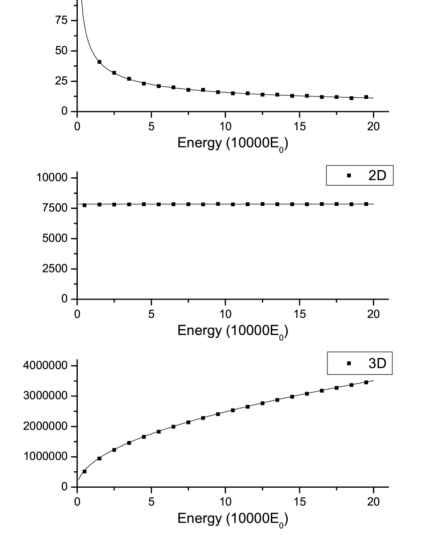
Figure 1:  List plots (dots) of Table 1, which approximate the density of states versus energy curve (solids) $n(E)=\mathrm{d}N/\mathrm{d}E$. $n_{\mathrm{1D}}(E)\propto E^{-1/2}$, $n_{\mathrm{2D}}(E)=\mathrm{const}$ and $n_{\mathrm{3D}}(E)\propto E^{1/2}$.

Below we use $F_{\mathrm{1D}}(t)$ to find the level degeneracies in 2D and 3D. Following Eq. (9), the degeneracies are

$$d_{\mathrm{2D}}(E) = [t^{E}]\,F_{\mathrm{1D}}^{2}(t),$$ (21)

$$d_{\mathrm{3D}}(E) = [t^{E}]\,F_{\mathrm{1D}}^{3}(t).$$ (22)

Unfortunately, series like $F_{\mathrm{1D}}(t)$ does not have a known explicit sum. Thanks to the advanced math softwares like Mathematica, we can use a computer to perform the evaluation. Mathematica’s “CoefficientList” function can extract the coefficients in the expansion of Eqs. (20-22). Then we are able to count the total number of states whose energies fall into the interval $[E_{1},E_{2}]$. Table 1 gives a detailed list of number of states within certain energy intervals for a 1D, 2D and 3D free particle, respectively. The list plots of the number of states are further presented in Fig. 1. There are totally $20$ energy intervals and each interval has a length of $10000$. Since the interval length is far more than the minimum separation between energy levels, the quasi-continuous approximation is valid and the plots will reflect approximately the dependence of density of states on the energy. A comparison between the discrete number of states and the continuous density of states is made in Fig. 1 (depicted as dots and solid lines, respectively). It can be seen that the exact numbers of states derived by a GF approach comply well with $n_{\mathrm{1D}}(E)\propto E^{-1/2}$, $n_{\mathrm{2D}}(E)=\mathrm{const}$ and $n_{\mathrm{3D}}(E)\propto E^{1/2}$.

- (1) Herbert S. Wilf, Generatingfunctionology (A K Peters, Ltd., 2006), 3rd ed.
- (2) See, for example, Kerson Huang, Introduction to Statistical Physics (CRC Press, 2001)
- (3) See, for example, Alan V. Oppenheim et al., Signals and Systems (Prentice Hall, 1996), 2nd ed.
- (4) It is commonly used in probability theory. See, for example, Athanasios Papoulis and S. Unnikrishna Pillai, Probability, Random Variables and Stochastic Processes (McGraw-Hill, 2002), 4th ed.
- (5) David J. Griffiths, Introduction to Quantum Mechanics (Benjamin Cummings, 2004), 2nd ed.
- (6) If an element in the tuple corresponds to a level of degeneracy , that tuple should be counted for times.
- (7) Assume the energy levels are quantized so that their separations are multiples of some unit. That is usually the case in a simple quantum system.
- (8) The spin degeneracies are excluded from the discussion.
- (9) See, for example, Charles Kittel, Introduction to Solid State Physics (Wiley, 2004), 8th ed.