Radio loud AGN and the $L_{X}-\sigma$ relation of galaxy groups and clusters

Abstract

We use the ROSAT All-Sky Survey to study the X-ray properties of a sample of 625 groups and clusters of galaxies selected from the Sloan Digital Sky Survey. We stack clusters with similar velocity dispersions and investigate whether their average X-ray luminosities and surface brightness profiles vary with the radio activity level of their central galaxies. We find that at a given value of $\sigma$, clusters with a central radio AGN have more concentrated X-ray surface brightness profiles, larger central galaxy masses, and higher X-ray luminosities than clusters with radio-quiet central galaxies. The enhancement in X-ray luminosity is more than a factor of two, is detected with better than 6$\sigma$ significance, and cannot be explained by X-ray emission from the radio AGN itself. This difference is largely due to a subpopulation of radio-quiet, high velocity dispersion clusters with low mass central galaxies. These clusters are underluminous at X-ray wavelengths when compared to otherwise similar clusters where the central galaxy is radio-loud, more massive, or both.

1 introduction

There is increasing evidence that the majority of radio-loud AGN at low redshift may be triggered by the accretion of hot gas. Using a sample of 625 nearby groups and clusters, Best et al. (2007) showed that the galaxies located closest to the centres of the clusters are more likely to host a radio-loud AGN than other galaxies of similar stellar mass. Allen et al. (2006) analyzed Chandra X-ray images of nine nearby X-ray luminous elliptical galaxies and showed that the jet power is tightly correlated with the Bondi accretion rate onto the central black hole as estimated from the observed gas temperature and density profiles.

It is also now recognized that the ‘over-cooling problem’ at the centre of many galaxy clusters could be solved if radio-loud AGN can heat surrounding gas. Direct evidence of AGN heating came with the discovery of X-ray cavities in the hot intracluster medium of a number of clusters and groups (Boehringer et al., 1993; Churazov et al., 2000; Fabian et al., 2000; McNamara et al., 2000; Blanton et al., 2003; Gitti et al., 2007). Some of these cavities coincide with extended lobes of radio emission produced by an AGN in the central cluster galaxy. The observations suggest that relativistic radio plasma displaces the X-ray emitting gas, generating turbulence and wave activity which heat the intracluster medium (ICM).

AGN feedback may also explain why low-temperature clusters are less X-ray luminous than predicted by a homologous scaling of the properties of hotter and more massive systems (Nath & Roychowdhury, 2002; Best et al., 2007). The energy available from the central AGN depends primarily on black hole accretion rate. In low-mass groups, it can be comparable to the total gravitational binding energy of the X-ray emitting gas, whereas high-mass clusters will be less strongly affected. As a result, relations such as $L_{X}-T_{X}$ (X-ray luminosity vs temperature) and $L_{X}-\sigma$ (X-ray luminosity vs velocity dispersion) may be modified by radio-source heating. At smaller scales, AGN feedback may play an important role in the formation and evolution of galaxies. Recent work has demonstrated that it can plausibly explain the exponential cutoff at the bright end of the galaxy luminosity function, as well as the ‘down-sizing’ of galactic star-formation activity at recent cosmic epochs (Croton et al., 2006; Bower et al., 2006; Kang et al., 2006).

It may be that hot gas accretion, AGN triggering, reheating of ambient gas, and suppression of AGN activity occur in a cycle. Accretion onto the central black hole may cause an outburst which removes the fuel supply for further radio activity. Without AGN feedback, the ICM reverts to the state that triggered the outburst (Churazov et al., 2005). Although this picture is attractive, it remains to be verified in detail. We do not know the necessary conditions to trigger or to quench radio activity. We also do not understand the extent to which the global X-ray properties of the gas are modified by AGN feedback(e.g. Rizza et al., 2000; Omma & Binney, 2004; Nusser & Silk, 2008). Only a few nearby clusters have deep enough X-ray images to reveal low-density cavities and permit the energetics of the gas to be studied in a spatially resolved fashion. If we wish to study how the global state of the X-ray gas is linked to AGN activity in the central galaxy, we are forced to adopt a more statistical approach.

It has long been known that the radio activity of cluster central galaxies is linked with the cooling flow or “cool core” phenomenon (Burns, 1990; Fabian, 1994). This is the fact that many but not all massive clusters show a strong central peak in X-ray surface brightness, almost always coincident with the brightest cluster galaxy (BCG), within which the directly inferred cooling time is less than the Hubble time. The fraction of cool-core clusters with a radio-loud BCG is much higher than the fraction in the rest of the population. Furthermore, because the cores add significantly to cluster luminosity and reduce the emission-weighted temperature, cool-core clusters fall systematically to one side of many of the X-ray scaling relations for clusters, e.g. the $L_{X}-T_{X}$ and $L_{X}-\sigma$ relations(Fabian et al., 1994; O’Hara et al., 2006; Chen et al., 2007). Thus, in clusters of given velocity dispersion (or mass), cool cores tend to be associated with enhanced X-ray luminosity, with massive central BCGs, and with radio-loud BCGs. Given that the probability of radio activity increases with BCG mass(Best et al., 2005), that both BCG mass and cluster X-ray luminosity increase with cluster mass(Edge & Stewart, 1991), and that central black hole mass correlates tightly with galaxy mass(Tremaine et al., 2002), it seems clear that radio activity is tightly related to both black hole mass and the presence of a cooling hot atmosphere which can provide fuel. The exact causal relation between these phenomena remains unclear, however, and recent observational studies of lower mass systems appear, at least superficially, in conflict with the trends established for relatively massive clusters [e.g. compare Croston et al. (2005) and Jetha et al. (2007) with the above references].

In this paper, we provide improved statistics for the relationship between cluster properties, both X-ray and optical, and the radio activity of their BCGs. We use a low redshift ($z<0.1$) sample of 625 groups and clusters with carefully controlled BCG identifications. These were selected by von der Linden et al. (2007) from the Sloan Digital Sky Survey(SDSS, York et al., 2000). Radio properties of these BCGs were determined following Best et al. (2005), who cross-matched the galaxies with the National Radio Astronomy Observatory Very Large Array Sky Survey (NVSS, Condon et al., 1998) and the Faint Images of the Radio Sky at Twenty Centimeters Survey (FIRST, Becker et al., 1995). By combining these two radio surveys, the identification of radio galaxies is both reasonably complete ($\sim 95$ per cent) and highly reliable ($\sim 99$ per cent). Radio-loud AGN are then separated from star-forming galaxies with detectable radio emission on the basis of 4000Å break strength(Best et al., 2005).

The sky coverage of this cluster sample is $\sim 4000$ square degrees. The only X-ray survey with enough sky coverage to provide a reasonable match is the ROSAT All-Sky survey(RASS). Because the RASS is quite shallow, relatively few individual groups and clusters have sufficient X-ray flux for unambiguous detection, particularly at low velocity dispersion. The mean flux of such objects can be detected, however, by stacking their X-ray images (e.g. Bartelmann & White, 2003; Shen et al., 2006; Dai et al., 2007; Rykoff et al., 2008). Such stacking avoids selection biases that can occur if one analyses samples in which only the most X-ray luminous systems are detected. The limited resolution of RASS maps and our stacking strategy, make it difficult to study the structure of the ICM in detail, but we will see that concentration differences, reflecting the presence of cool cores, are nevertheless detectable.

Our paper is organized as follows. In Section 2, we introduce our sample of groups and clusters and describe their radio properties. In Section 3, we describe our X-ray detection techniques, both our method for detecting individual groups and clusters and our stacking technique. In section 4, we study and compare the X-ray properties of clusters, emphasising how the $L_{X}-\sigma$ relation and the surface brightness profiles of clusters vary with the radio properties of their BCGs. We discuss the contribution of the radio AGN to the total X-ray emission in Section 5.1, while in Section 5.2, we discuss how the $L_{X}-\sigma$ relation of clusters depends on the stellar properties of their BCGs. We present our conclusions in Section 6.

2 sample

We use the sample of groups and clusters of galaxies described in von der Linden et al. (2007), which is drawn from the C4 cluster catalogue of the SDSS Data Release 3 (Miller et al., 2005). The clusters lie in the redshift range $0.02\leq z\leq 0.1$. Von der Linden et al. developed improved algorithms for identifying the brightest galaxy (the BCG) and for measuring the velocity dispersion in each group or cluster. The velocity dispersion algorithm is designed to limit the effects of neighbouring groups and clusters. Clusters and groups with very few galaxies are also discarded. The velocity dispersion $\sigma$ is measured within the virial radius $R_{200}$. The radio properties of the BCGs are taken from the catalogue of Best et al. (2005), which has been updated to the SDSS data release 4.

The final sample includes 625 groups and clusters, with velocity dispersion spanning the range from $\sim 200\,\>{\rm km}\,{\rm s}^{-1}$ to over 1000 $\>{\rm km}\,{\rm s}^{-1}$ (see von der Linden et al. 2007 for more details). 134 out of the 625 BCGs have radio fluxes larger than 5 mJy and are identified as radio-loud AGN. Five BCGs have radio fluxes which exceed 5 mJy but are clearly a result of star formation activity. There are 433 BCGs without a radio source brighter than 5mJy. The radio properties of the remainder are unknown because they lie outside the area covered by FIRST. Henceforth, we will refer to a group or cluster as ‘radio-loud’ if its BCG has been identified as a radio-loud AGN, and ‘radio quiet’ if it is known to contain no radio source brighter than 5mJy. There are 134 radio-loud and 433 radio-quiet clusters in our sample. The fraction of radio-loud clusters in our sample is smaller than the fraction of clusters usually quoted as having cooling cores($\sim 40\%$ according to Peres et al., 1998). This may well be a selection effect since X-ray selected cluster samples are biased towards massive and X-ray luminous systems.

In figure 1 we show histograms of velocity dispersion $\sigma$ and redshift $z$ for radio-loud and radio-quiet clusters. The two redshift distributions are very similar. The radio-loud clusters have slightly higher velocity dispersions than the radio-quiet objects. The median $\sigma$ of radio-loud clusters is 428 $\>{\rm km}\,{\rm s}^{-1}$, with 16 and 84 percentiles at 277 and 595 $\>{\rm km}\,{\rm s}^{-1}$ respectively. For radio-quiet clusters, the corresponding $\sigma$ values are 392, 252 and 583 $\>{\rm km}\,{\rm s}^{-1}$. The figure also shows $\sigma$ and $z$ distributions for a control sample of radio-quiet clusters (dashed line). This was constructed by choosing the radio-quiet cluster closest in $\sigma$ and $z$ to each radio-loud cluster (see Section 4.2). This matching procedure was introduced in order to minimize possible observationally induced biases when comparing the two samples.

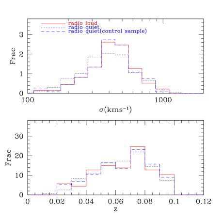
Figure 1: Velocity dispersion and redshift distributions for all radio-loud clusters (solid histograms), for all radio-quiet clusters (dotted histograms) and for our matched control sample of radio-quiet clusters (dashed histograms).

3 X-ray detection

We use the RASS to study the X-ray properties of our sample of groups and clusters. The RASS mapped the sky in the soft X-ray band (0.1$-$2.4keV) with exposure time varying between 400 and 40,000s, depending on direction on the sky. The resolution of the RASS images is 45 arcsec. Two source catalogues were generated based on RASS images through a maximum-likelihood (ML) search algorithm: the bright source catalogue (Voges et al., 1999) and the faint source catalogue (Voges et al., 2000). However, these source catalogues are not optimized for extended sources. An extended source is likely to be deblended into several pieces by the ML search algorithm.

There are carefully selected samples of X-ray clusters constructed from the RASS data, e.g. the Northern ROSAT All-Sky Galaxy Cluster Survey (NORAS, Böhringer et al., 2000) and the ROSAT-ESO Flux-Limited X-Ray Galaxy Cluster Survey (REFLEX, Böhringer et al., 2004)). The REFLEX clusters, which have a completeness of $\geq 90\%$ at the flux limit of $3\times 10^{-12}\rm{erg\,cm^{-2}\,s^{-1}}$, are mainly located in the southern sky ($\delta\leq 2.5$) and have little overlap with our SDSS clusters. For the NORAS clusters, the completeness is estimated to be $\sim 50\%$ at an X-ray flux of $3\times 10^{-12}\rm{erg\,cm^{-2}\,s^{-1}}$ (Böhringer et al., 2004).

Our sample of groups and clusters has been selected from an optical galaxy catalogue. The centre of the cluster (taken to be the position of the BCG) and the virial radius of each cluster have already been determined. We use this extra information when studying their X-ray properties. We first check whether the position of the BCG of each cluster is consistent with a peak in X-ray emission (Section 3.1). We then optimize the growth curve analysis algorithm of Böhringer et al. (2004) to detect the X-ray properties of our clusters individually (Section 3.2). Finally, we develop a stacking algorithm to measure the mean X-ray properties of clusters as a function of their optical properties, independent of the detection limit of the RASS (Section 3.3).

3.1 Finding the X-ray centre of the clusters

Before the X-ray luminosity of a cluster can be measured, the position of its centre must be determined. In the optical, the position of the BCG is usually taken to define the cluster centre. However, this position may be offset from the peak of the X-ray emission (e.g. Dai et al., 2007; Koester et al., 2007). In order understand whether such offsets are generic for clusters in our sample, we have developed an algorithm to determine the X-ray centre of a cluster.

First, the ML search algorithm used to generate the ROSAT source catalogue is applied to the RASS images (Voges et al., 1999). Sources with detection likelihood $L>7$ in the $0.5-2.0$ keV band are retained. Although an extended source is frequently de-blended into several pieces by this algorithm, the central peak is always identified. We match the position of each BCG with the ML detections using a tolerance of 5 arcmin in radius. X-ray sources found within this radius are considered as candidate X-ray centres. We find that 210 clusters have X-ray sources within a 5 arcmin radius and some clusters have several candidate X-ray centres. We then exclude candidates which are clearly not associated with the clusters by eye. If a point source is detected within the 5 arcmin search radius but significantly offset from the BCG, we assume that the source is a contaminant and is not part of the cluster. We show such an example in Fig. B1 of Appendix B. For clusters that still have more than one candidate X-ray centre, we pick the closest one. Most of the sources we identified as the X-ray centres of clusters have extension likelihood greater than zero. This confirms that the X-ray emissions we identified are from the extended ICM rather than from point-like AGN. As we will show in Section 5.1, the X-ray emission from radio AGN in the soft X-ray bands is expected to be much weaker than the X-ray emission we measure. Our final sample of clusters with identified X-ray centres contains 157 objects.

In Figure 2 we plot the offset between X-ray centre and optical centre (i.e. the BCG position) for these 157 clusters. The upper panel shows the offset in units of arcmin, while the lower panel shows the corresponding projected physical distance at the redshift of BCG. As can be seen, the X-ray centre is consistent with the BCG position in most cases. The typical offset is less than 2 armin ($\sim$ 3 RASS pixels). This corresponds to a physical distance of around 50 kpc and so is consistent with the results of Katayama et al. (2003).

Figure 2: A histogram of the offset between BCG and X-ray centre. The upper panel shows the offset in units of arcmin, while the lower panel shows the offset in units of kpc.

Since the BCG positions are, in general, consistent with the X-ray centres, we will assume that the BCGs mark the centres of those clusters which are too faint to determine an X-ray centre directly with our algorithm.

3.2 Measuring the X-ray luminosity

After the centre of each cluster has been determined, we use a growth curve analysis to count the number of photon events as function of radius and so to evaluate the cluster count rate.

The background of each cluster is estimated from a centred annulus with inner radius $R_{200}$ and width 6 arcmin. To exclude contamination of this background estimate by discrete sources, we mask out all ML-detected ($L>7$) sources inside this annulus. The surface brightness of the background is then calculated using the formula

$$\mu=\frac{\sum_{i=1}^{N}\frac{1}{t_{i}}}{S},$$ (1)

where the sum is over the photon events, $t_{i}$ is the effective exposure time at each photon position, and $S$ is the effective area of the annulus after the contaminating sources are masked out.

The count rates within $R_{200}$ may also be contaminated by discrete X-ray sources unassociated with intracluster X-ray emission. As above, we therefore mask out all the ML-detected ($L>7$) point sources that are located more than 2.25 arcmin (3 image pixels) from the X-ray centre. As already mentioned, an extended source is often detected multiple times by the ML algorithm. We therefore visually inspect all the ML sources and determine whether they are contaminants or part of the X-ray emission from the cluster. We show an example of this process in Fig. B2 of Appendix B.

The cumulative source count rate as a function of radius is calculated by integrating the source counts in concentric rings and subtracting the background contribution. We integrate the source count rate to the X-ray extension radius $R_{X}$. We determine this radius in two different ways, as described in Böhringer et al. (2000). The first chooses the radius where the increase in source signal is less than the 1$\sigma$ uncertainty in the count rate. The other is the plateau-fitting method, where the slope of the plateau (in units of count rate per arcmin) is less than 1 percent. These two methods give consistent results for clusters where the count rate profile can be determined with high S/N. For low S/N clusters, we choose the better determination of $R_{X}$ by visually checking the cumulative count rate profile. A source is said to have a significant X-ray detection if the counts within $R_{X}$ are three times larger than the Poisson fluctuation in the photon counts. We detect 159 galaxy clusters individually according to this criterion.

To convert the count rates into X-ray fluxes, we assume that the X-ray emission has a thermal spectrum with temperature $T$, that the cluster gas has metal abundance equal to a third of the solar value (Raymond & Smith, 1977) and that interstellar absorption can be inferred from the Galactic hydrogen column density (Dickey & Lockman, 1990). The gas temperature $T$ is assumed to follow the empirical scaling relation measured by White et al. (1997),

$$T=\left(\frac{\sigma}{403\>{\rm km}\,{\rm s}^{-1}}\right)^{2}.$$ (2)

One might question whether this assumption is robust. Most studies of the $T-\sigma$ relation find that it does not depart significantly from the virial theorem expectation ($T\propto\sigma^{2}$), even for low-mass galaxy groups (e.g. Girardi et al., 1996; Wu et al., 1999; Mulchaey, 2000; Xue & Wu, 2000). We further note that a variation in temperature of 50 percent makes less than a 5 percent difference to the flux estimate for most of our clusters. Throughout this paper we adopt a concordance $\Lambda$CDM cosmology with $H_{0}=70\>{\rm km}\,{\rm s}^{-1}\,{\rm Mpc}^{-1}$, $\Omega_{0}=0.3$, and $\Omega_{\Lambda}=0.7$.

For some clusters, the total X-ray flux will exceed the flux measured within the extension radius $R_{X}$. To estimate the flux that is missed outside $R_{X}$, we adopt a $\beta$-model surface brightness distribution $I_{X}(R)$ with $\beta=2/3$,

$$I_{X}(R)=I_{0}(1+\frac{R^{2}}{R_{c}^{2}})^{-3\beta+0.5},$$ (3)

where $I_{0}$ is the central surface brightness and $R_{c}$ is the core radius and is assumed to be proportional to $R_{200}$, with $R_{c}=0.14R_{200}$ for radio-loud clusters and $R_{c}=0.18R_{200}$ for radio-quiet clusters. The extension correction factor $f_{E}$ is then defined as

$$f_{E}=\frac{\int_{0}^{R_{200}}I_{X}(R)RdR}{\int_{0}^{R_{X}}I_{X}(R)RdR}.$$ (4)

The exact values of $R_{c}$ and $\beta$ are far from certain for each individual cluster. As a result, the X-ray luminosities of clusters with large correction factors $f_{E}$ have larger errors. To account for this effect, we assume that the correction factor $f_{E}$ has an uncertainty of 0.1$f_{E}$. We note that for a few clusters with sufficiently high S/N, we can apply a $\beta$ model fit and derive the extension correction factor $f_{E}$. We find answers that are consistent with the estimates using Equ. (4) with an uncertainty of $\sim 10$%. The error on our estimate of $L_{X}$ for each cluster thus has two terms: the error of the flux estimation inside $R_{X}$ and the error on the correction factor $f_{E}$.

The X-ray properties of the 159 clusters that are individually detected in RASS are listed in Appendix A.

3.3 Stacking Analysis

The clusters that are individually detected in the RASS are biased to the nearest and most X-ray luminous systems at each velocity dispersion. We can obtain an unbiased estimate of the average X-ray luminosity of our clusters by stacking objects with similar optical properties. We describe our stacking algorithm below.

We divide the clusters into bins of velocity dispersion with a width of $\sim 100\>{\rm km}\,{\rm s}^{-1}$. Within each velocity dispersion bin, the angular size of the clusters varies substantially because of the spread in redshift. (Recall that $R_{200}$ is proportional to $\sigma$.) We centre each cluster image on the X-ray centre if this has been identified (see Section 3.1) and on the BCG otherwise. Before stacking the images, we scale them all to the same size in units of $R_{200}$ and mask contaminating sources in the same way as in our analysis of individual clusters. The background is estimated as the average flux inside an annulus with inner radius $R_{200}$ and outer radius $1.3R_{200}$. The remaining steps in the detection algorithm (determining the extension radius $R_{X}$ and count rate) parallel those used for individual clusters. A stacked image is said to have a robust X-ray detection if the number of source photons within $R_{X}$ is also three times larger than the Poisson fluctuation in the photon counts.

For a stack of $N$ clusters with individual X-ray luminosities $L_{X,i}$, redshifts $z_{i}$, average Galactic hydrogen columns $N_{H,i}$ and average RASS effective exposure times $t_{i}$, the number of source photons that should be detected in the RASS, $N_{s}$, is

$$N_{s}=\sum_{i=1}^{N}{L_{X,i}~{}g(N_{H,i},z_{i})t_{i}}\,,$$ (5)

where $g(N_{H,i},z_{i})$ is a function which converts the bolometric X-ray luminosity to observed count rate. Since the X-ray luminosities of the sources in a stack are similar, the weighted average X-ray luminosity of the stack can be defined as

$$L_{X,S}=\frac{N_{s}}{\sum_{i=1}^{N}{g(N_{H,i},z_{i})t_{i}}}.$$ (6)

We fit the surface brightness profile of each stack with a $\beta$ model to make the extension correction, and we correct the X-ray luminosity to the value expected within $R_{200}$ (see Section 4.2.1).

4 X-ray properties of the clusters

In this section, we investigate how the X-ray properties of the clusters depend on the radio properties of their central BCGs. We focus on the comparison of the $L_{X}-\sigma$ relations of radio-loud and radio-quiet clusters. We first show results for clusters that were detected individually in the X-ray images (Section 4.1). We then present results for stacked cluster samples (Section 4.2).

4.1 Results for individual X-ray detections

4.1.1 Detected fraction

As we showed in Section 3.2, only $\sim 25$ percent (159 out of 625) of our clusters are individually detected in the RASS. The solid histogram in figure 3 shows the detected fraction as function of velocity dispersion. As expected, the detected fraction is higher for higher velocity dispersion clusters. It increases from less than 15 per cent for groups with $\sigma<400\,\>{\rm km}\,{\rm s}^{-1}$ to more than 50 percent for clusters in the highest velocity dispersion bin.

We find that 55 of the 134 radio-loud clusters and 88 of the 433 radio-quiet clusters are detected. The detected fractions as function of velocity dispersion for these two sub-samples are plotted in Fig. 3. As can be seen, the detected fraction is systematically higher for radio-loud than for radio-quiet clusters in all the velocity dispersion bins.

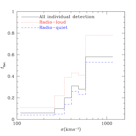
Figure 3: The fraction of clusters with individual X-ray detections as a function of velocity dispersion. The solid histogram shows the result for the whole sample, while the dotted and dashed histograms show results for radio-loud and radio-quiet clusters, respectively.

4.1.2 $L_{X}-\sigma$ relation for clusters with individual X-ray detections

Table 1: Fitting parameters for various $L_{X}-\sigma$ relations. $a$ and $b$ are the fitting parameters of equation (7). $N$ is the number of objects in each sample. For stacked samples, $N$ is given as $N1/N2$, where $N1$ is the number of stacks while $N2$ is the total number of clusters in the sample. $M$ is the median BCG stellar mass. $b^{\prime}$ gives the zero-points obtained if the $L_{X}-\sigma$ relations are refit requiring the slope $a$ to be 2.97 for the low BCG mass and low BCG mass radio-quiet samples and to be 4.40 for the other stacked samples.

Sample	$a$	$b$	$N$	$M(\rm{M\odot})$	$b^{\prime}$
Individual, all	$4.39\pm 0.32$	$-0.530\pm 0.037$	159	$1.82\times 10^{11}$	$-$
Individual, radio-loud	$4.48\pm 0.61$	$-0.535\pm 0.058$	55	$2.09\times 10^{11}$	$-$
Individual, radio-quiet	$4.50\pm 0.44$	$-0.530\pm 0.056$	88	$1.78\times 10^{11}$	$-$
Stack, radio-loud	$4.40\pm 0.53$	$-0.600\pm 0.099$	8/134	$1.66\times 10^{11}$	$-0.600\pm 0.032$
Stack, control radio-quiet	$4.07\pm 0.24$	$-0.935\pm 0.049$	8/134	$1.35\times 10^{11}$	$-0.942\pm 0.045$
Stack, low BCG mass	$2.88\pm 0.17$	$-1.150\pm 0.055$	7/217	$7.76\times 10^{10}$	$-1.151\pm 0.033$
Stack, intermediate BCG mass	$4.58\pm 0.56$	$-0.712\pm 0.116$	8/208	$1.35\times 10^{11}$	$-0.703\pm 0.037$
Stack, high BCG mass	$4.16\pm 0.44$	$-0.638\pm 0.072$	8/200	$2.14\times 10^{11}$	$-0.646\pm 0.030$
Stack, radio-loud, low BCG mass	$4.17\pm 0.74$	$-0.572\pm 0.104$	6/67	$1.20\times 10^{11}$	$-0.563\pm 0.041$
Stack, radio-loud, high BCG mass	$4.49\pm 0.47$	$-0.650\pm 0.072$	6/67	$2.14\times 10^{11}$	$-0.651\pm 0.048$
Stack, radio-quiet, low BCG mass	$3.07\pm 0.21$	$-1.160\pm 0.053$	7/219	$8.32\times 10^{10}$	$-1.162\pm 0.032$
Stack, radio-quiet, high BCG mass	$4.25\pm 0.44$	$-0.704\pm 0.088$	8/214	$1.74\times 10^{11}$	$-0.711\pm 0.040$

In figure 4 we plot bolometric X-ray luminosity $L_{X}$ as function of velocity dispersion $\sigma$ for clusters with individual X-ray detections. $L_{X}$ is in units of $L_{X}/10^{44}\rm{erg\,cm^{-2}\,s^{-1}}$($L_{44}$) and velocity dispersion in units of $\sigma/500\>{\rm km}\,{\rm s}^{-1}$($\sigma_{500}$).

Figure 4: The $L_{X}-\sigma$ relation of clusters that are individually detected in the RASS. The solid line shows the linear fit of equation (8). For comparison, the dotted line shows the fit obtained by Ortiz-Gil et al.(2004) for REFLEX clusters.

We use the BCES orthogonal distance regression method (Akritas & Bershady, 1996) to fit a linear relation between $\,{\rm log}\,L_{44}$ and $\,{\rm log}\,\sigma_{500}$,

$$\,{\rm log}\,L_{44}=a\,{\rm log}\,\sigma_{500}+b.$$ (7)

This fitting method takes into account the observational errors on both variables and the intrinsic scatter in the relation. The determination of the error on $L_{X}$ has been described in section 3.2, while the error on $\sigma$ is given by von der Linden et al. (2007). The best fitting relation is

$$\,{\rm log}\,L_{44}=(4.39\pm 0.32)\,{\rm log}\,\sigma_{500}+(-0.530\pm 0.037),$$ (8)

and is shown as solid line in Fig. 4. The fitting parameters are also listed in Table 1. For comparison, we also plot the $L_{X}-\sigma$ relation derived for REFLEX clusters by Ortiz-Gil et al. (2004) using the orthogonal distance regression method (dotted line). As we can see, the slopes of two fitting relations are consistent with each other within the 1-$\sigma$ uncertainty. The zero-point of our relation is slightly higher. This difference is caused by the fact that Ortiz-Gil et al. adopted a lower value of $R_{c}$ for the extension correction [$R_{c}\propto L_{x}^{0.28}$, Equ. (6) of Böhringer et al. (2000)].

We show $L_{X}-\sigma$ relations for the sub-samples of detected radio-loud and radio-quiet clusters in the left and right panels of figure 5 respectively. The BCSE orthogonal regression method is again used to fit a linear relation between $\,{\rm log}\,L_{44}$ and $\,{\rm log}\,\sigma_{500}$. The results are

$$\,{\rm log}\,L_{44}=(4.48\pm 0.61)\,{\rm log}\,\sigma_{500}+(-0.535\pm 0.058),$$ (9)

for radio-loud clusters and

$$\,{\rm log}\,L_{44}=(4.50\pm 0.44)\,{\rm log}\,\sigma_{500}+(-0.530\pm 0.056),$$ (10)

for radio-quiet clusters. These two relations are plotted as solid lines in figure 5. The relation for the cluster sample as a whole [Equ. (8)] is shown as a dotted line in each panel for comparison. Again, the fitting parameters are listed in Table 1.

Even though radio-loud clusters are more frequently detected in the X-ray than radio-quiet objects, the two relations in Figure 4 are similar. As we demonstrate in the next section, this is simply a selection effect. The majority of individually detected clusters are just above the X-ray detection limit in both samples. Since the redshift distributions of the two types of cluster are similar (Fig. 1), this forces the mean $L_{X}-\sigma$ relations of detected objects to be nearly the same.

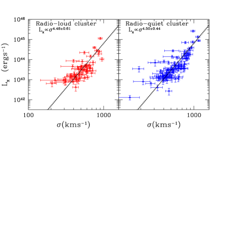
Figure 5: The $L_{X}-\sigma$ relation of radio-loud (left panel) and radio-quiet (right panel) subsamples of clusters. The solid line in each panel is the best linear fit [equations (9) and (10)], while the dotted line shows the fit to the sample as a whole for comparison [equation (8)].

4.2 Results for the stacks

We stack the radio-loud and the radio-quiet clusters independently. Clusters with unclear radio properties are excluded from this analysis.

Radio-loud clusters with $\sigma$ in the range $300-900\>{\rm km}\,{\rm s}^{-1}$ are stacked in velocity dispersion bins with width $100\>{\rm km}\,{\rm s}^{-1}$. Smaller groups with $\sigma<300\>{\rm km}\,{\rm s}^{-1}$ and bigger clusters with $\sigma>900\>{\rm km}\,{\rm s}^{-1}$ are split into two separate velocity dispersion bins. Our sample of 134 radio-loud clusters then splits into 8 stacks.

As described above, we create a control sample of 134 radio-quiet clusters selected to have the same $\sigma$ and $z$ distributions as the radio-loud sample. This control sample is generated from the full sample of 433 radio-quiet clusters by picking the radio-quiet cluster that is most similar in $z$ and $\sigma$ to each of the radio-loud clusters. These radio-quiet clusters are then stacked in exactly the same way as the radio-loud clusters. More specifically , for $i$-th radio-loud cluster that is included in the $k$-th radio-loud stack, the corresponding $i$-th control radio-quiet cluster is stacked into $k$-th radio-quiet stack. X-ray detections are obtained for all 16 stacks.

4.2.1 Surface brightness profiles of the clusters

We show radial surface brightness profiles for each of our eight different velocity dispersion stacks in figure 6. The radio-loud clusters are plotted as triangles while the control radio-quiet clusters are plotted as squares. Surface brightness is given in units of photon counts per unit area per second and is plotted as a function of the scaled radius $R/R_{200}$. The error in the surface brightness in each radial bin is estimated from the Poisson fluctuations of the photon counts. As we can see, after stacking, the S/N of the surface brightness profiles in all the velocity dispersion bins is sufficiently good to enable model fitting to be carried out.

We use a $\beta$ model [Equ. (3)] to fit the surface brightness profile for each stack. To reduce the number of free parameters, we fix $\beta=2/3$ and estimate $R_{c}$ and $I_{0}$ by minimizing $\chi^{2}$. We show the best fitting results as solid and dashed lines in each panel for radio-loud and radio-quiet clusters respectively. The best fitting value of $R_{c}$ for each profile is quoted as a label in each panel of Fig. 6. Except for the two lowest velocity dispersion bins, radio-loud clusters have more concentrated luminosity profiles (smaller $R_{c}$) than radio-quiet clusters.

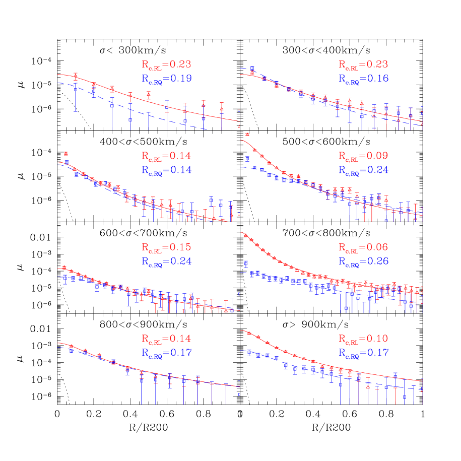
Figure 6: Surface brightness profiles for stacks of clusters in 8 velocity dispersion bins. Triangles show results for radio-loud clusters while squares are for the control sample of radio-quiet clusters. The solid and dashed lines show best fit $\beta$ models for radio-loud and radio-quiet clusters respectively. The dotted curves show the contribution to the X-ray emission predicted to come from the radio AGN itself (see the text in Section 5.1 for details).

We show the best fit values of $R_{c}$ as a function of velocity dispersion in figure 7. Radio-loud and radio-quiet clusters are represented by triangles and squares, respectively. The median $R_{c}$ of the radio-loud clusters is 0.14$R_{200}$, whereas the median for radio-quiet clusters is 0.18$R_{200}$. These two median values are shown as horizontal lines in Fig. 7. The core radii of our stacked clusters are consistent with the studies of individual clusters by Neumann & Arnaud (1999). These authors found $R_{c}\sim 0.1-0.2R_{200}$ for clusters with $\beta\sim 2/3$. We note that uncertainties in the centroids of individual cluster will broaden the X-ray core of the stacked profile (e.g. Dai et al., 2007). This effect is not significant in our study, however, since the centroids of most of our individual detected clusters (which contribute the bulk of the flux of the stacks) were identified before stacking(see Section 3.1). We find that if we stack only the clusters with individual detections, the median $R_{c}$ values are $0.14R_{200}$ and $0.17R_{200}$ for radio-loud and radio-quiet clusters respectively. The point-spread function of the ROSAT telescope also broadens the estimated core radii of the clusters, of course, particularly for low velocity dispersion clusters which typically have small angular size.

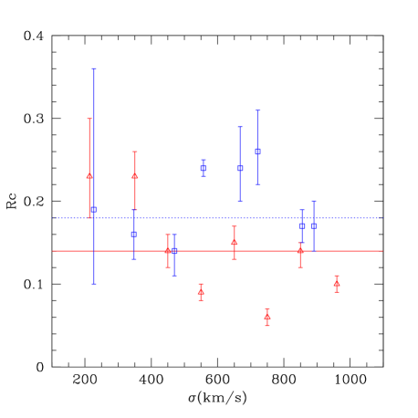
Figure 7: The best fit value of $R_{c}$ for surface brightness profiles of clusters stacked in 8 bins of velocity dispersion. Triangles and squares represent radio-loud and radio-quiet clusters respectively. $R_{c}=0.18R_{200}$ (solid line) and $R_{c}=0.14R_{200}$ (dotted line) are the median values of $R_{c}$ for the radio-loud and radio-quiet clusters respectively.

4.2.2 $L_{X}-\sigma$ relation for the stacks

In figure 8, we show the weighted average X-ray bolometric luminosity $L_{X,S}$[Equ. (6)] as a function of the average velocity dispersion $\sigma_{S}$ for our stacks of radio-loud and radio-quiet clusters. We use the BCSE orthogonal regression method to fit linear relations between $\,{\rm log}\,L_{X,S}$ and $\,{\rm log}\,\sigma_{S}$ weighted by the errors on both $L_{X,S}$ and $\sigma_{S}$. The error on $\sigma_{S}$ is estimated from the error on the mean value of $\sigma$ of the stacked clusters. Our result is

$$\,{\rm log}\,L_{44}=(4.40\pm 0.53)\,{\rm log}\,\sigma_{500}+(-0.600\pm 0.099)$$ (11)

for radio-loud clusters and

$$\,{\rm log}\,L_{44}=(4.07\pm 0.24)\,{\rm log}\,\sigma_{500}+(-0.935\pm 0.049)$$ (12)

for radio-quiet clusters. These relations are shown as solid lines in the left and right panels of Fig. 8 for radio-loud and radio-quiet clusters respectively. The parameters of the fits are also listed in Table 1. The $L_{X}-\sigma$ relation for the individually detected clusters [Equ. (8)] is shown as a dotted line in each panel for comparison. The $L_{X}-\sigma$ relation of the stacks of radio-loud clusters is very close to that for all individual detections (dotted line). This is a coincidence. If we stack only the individually detected clusters, we find a significantly higher $L_{X}$ at given $\sigma$ than predicted by Equ. (8) (the dotted line). This is because, at given $\sigma$, the mean $L_{X}$ of the stacked objects is higher than their median $L_{X}$. The latter is what is approximated by a linear fit in $\,{\rm log}\,\sigma$ – $\,{\rm log}\,L_{X}$ space.

The slopes of the $L_{X}-\sigma$ relations for the radio-loud and (control) radio-quiet clusters are consistent within the 1-$\sigma$ error, but their zero-points differ significantly. At given velocity dispersion, the average X-ray luminosity of radio-loud clusters is systematically higher than that of radio-quiet clusters. To demonstrate the significance of this effect, we fix the slope of both relations to be 4.17 [the error-weighted mean of the slopes in Equ. (11) and (12)], and then re-estimate their zero-points. The results are ($-0.591\pm 0.031$) for radio-loud clusters and ($-0.937\pm 0.044$) for radio-quiet clusters. At given velocity dispersion, the X-ray luminosity of radio-loud clusters is on average 2.2 times higher than that of radio-quiet clusters. The difference is significant at 6.4$\sigma$ and is consistent with our earlier result that the fraction of radio-loud clusters with individual X-ray detections is substantially higher than the corresponding fraction for radio-quiet clusters (Section 4.1.1). The difference is also comparable to the difference in normalization between cooling core and non-cooling core clusters found by Chen et al. (2007) using the $L_{X}-M$ relation ($M$ is cluster mass) .

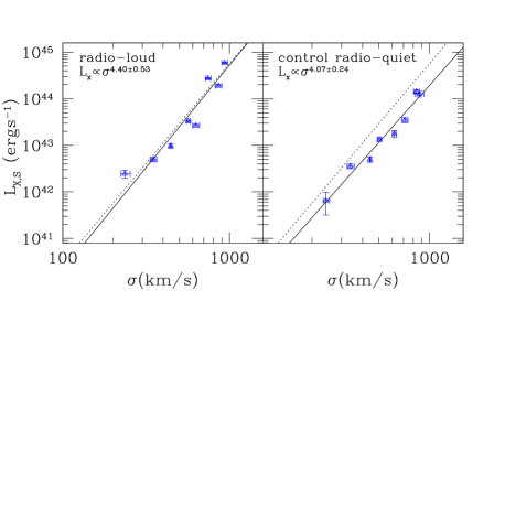
Figure 8: The average X-ray luminosity $L_{X,S}$ as a function of average velocity dispersion $\sigma_{S}$ for stacked clusters. The left and right panels show results for radio-loud and radio-quiet clusters respectively. The solid lines show the best linear fits to the relation between $\,{\rm log}\,L_{X,S}$ and $\,{\rm log}\,\sigma_{S}$ [Equ. (11) and Equ. (12)]. The $L_{X}-\sigma$ relation for all clusters with individual X-ray detections [Equ. (8)] is shown as a dotted line in each panel for comparison.

5 Discussion

The results presented above demonstrate that the X-ray properties of the ICM are correlated with the radio properties of the central BCGs. Clusters with radio-loud BCGs are more frequently detected in X-ray images. When we stack radio-loud and radio-quiet clusters with similar velocity dispersions and redshifts, we find that radio-loud clusters have more concentrated surface brightness profiles and higher average X-ray luminosities than their radio-quiet counterparts.

Up to now, we have not considered X-ray emission from the central radio AGN itself. If this emission were comparable to the X-ray emission from the ICM, all our results might be explained without any need to invoke a correlation between the radio AGN and the state of the intracluster gas. We estimate the X-ray emission from the AGN itself in Section 5.1.

Furthermore, we have not yet considered how X-ray and radio properties correlate with the stellar properties of BCGs. As shown by Best et al.(2005, 2007), radio-loud AGN occur more frequently in higher stellar mass BCGs, which also tend to be found in more X-ray luminous clusters(Edge & Stewart, 1991). The correlation between BCG stellar mass and cluster X-ray luminosity is two-fold. On the one hand, more massive clusters typically host higher mass BCGs(see top panel of Fig. 10). On the other hand, at given cluster mass (velocity dispersion), clusters with higher mass BGCs tend to be more regular and more concentrated(Bautz & Morgan, 1970), and such clusters tend to have higher X-ray luminosities(David et al., 1999; Ledlow et al., 2003). This morphology – BCG mass dependence appears related to the presence of the cool cores(Edge & Stewart, 1991). Thus, we may expect the mean stellar masses of the BCGs to differ between the radio-loud and radio-quiet clusters we have stacked above, and we may expect clusters stacked as a function of BCG mass to show similar differences in X-ray properties to our radio-loud and radio-quiet samples. In Section 5.2, we compare the stellar properties of the BCGs in our radio-loud and radio-quiet samples, and we stack clusters also as a function of BCG properties.

5.1 The X-ray emission from radio AGN

The X-ray luminosities of radio-loud AGN $L_{X,AGN}$ are correlated with their radio luminosities $L_{R}$ (e.g. Brinkmann et al., 2000; Merloni et al., 2003). Using the $L_{X,AGN}-L_{R}$ correlation for radio-loud AGN from the study of Brinkmann et al. (2000), we estimate X-ray luminosities for our sample of radio AGN ($L_{X,AGN}$) in the ROSAT $0.1-2.4\rm{keV}$ band. Here we assume that the distributions of radio flux and of X-ray photon energy are power laws, $S_{\mu}\sim\mu^{-0.5}$ and $N(E)\sim E^{-2}$ (see Brinkmann et al., 2000). We then compare our estimated values of $L_{X,AGN}$ with the $0.1-2.4\rm{keV}$ X-ray luminosities $L_{X,ICM}$ measured for our clusters within the radius $R_{X}$. The results are shown in figure 9. The top panel shows results for individually detected clusters; the bottom panel shows corresponding results for the stacked clusters. For the stacks, we estimate $L_{X,AGN}$ as the weighted average of the estimated X-ray luminosities of the central radio AGN.

As can be seen, the estimated X-ray luminosities of the radio AGN are typically a small fraction ($<5$ percent) of the total measured X-ray emission. The enhancement we measure in the X-ray luminosity of radio-loud clusters is more than a factor of 2 (Section 4.2). Thus, contamination of the X-ray emission by the radio AGN is at most a small part of the effect we measure.

One might also ask whether X-ray emission from the radio AGN might explain the more concentrated X-ray surface brightness profiles seen in figure 6. The dotted curve in each panel shows the predicted contribution of the radio AGN to the X-ray surface brightness profile. The $L_{X}-L_{R}$ relation of Brinkmann et al. (2000) was again used to estimate the X-ray luminosity of each radio AGN and a Gaussian PSF with FWHM = 1 arcmin was used to predict its count rate profile. These count rate profiles were then scaled and stacked in order to calculate the average AGN contribution to the profile of the stack. As we can see, this contribution is negligible even in the lowest velocity dispersion bin.

Figure 9: Comparison of the predicted X-ray emission from radio AGN($L_{X,AGN}$) to the total observed cluster emission ($L_{X,ICM}$) for our sample of radio-loud clusters. The AGN luminosity is estimated from the $L_{X}-L_{R}$ relation of Brinkmann et al.(2000). The top panel gives results for individually detected clusters, the bottom panel for our eight stacks of clusters. The dotted lines represent the relation $L_{X,AGN}=0.05L_{X,ICM}$.

5.2 The stellar properties of BCGs

In this section we investigate the relation between our results and the stellar properties of our BCGs, as characterised by their stellar mass and their concentration. The concentration is defined as $c\equiv R_{90}/R_{50}$. where $R_{90}$ and $R_{50}$ are the radii including 90 and 50 percent of the flux from a galaxy. It can be used as an indicator of galaxy morphology(Shimasaku et al., 2001). For early-type galaxies, the stellar mass correlates closely with the mass of the central supermassive black hole.

We first divide our radio-loud clusters into 8 velocity dispersion bins containing equal numbers of objects. The median stellar mass and concentration are then calculated for both radio-loud and control radio-quiet clusters in these 8 bins. In figure 10, we show these median values as a function of velocity dispersion. For both properties red triangles represent radio-loud clusters, while blue squares represent the radio-quiet clusters. The horizontal error-bars show the range of velocity dispersion for each bin, while the vertical error-bars link the 32 and 68 percentiles of the distribution in concentration and stellar mass.

Clearly, the stellar masses of BCGs correlate with the velocity dispersions of their host clusters; higher velocity dispersion clusters tend to have higher stellar mass BCGs. In addition, at given velocity dispersion, the stellar mass of radio-loud BCGs is systematically higher than that of radio-quiet objects. This mirrors the earlier finding of Best et al.(2005, 2007) that higher stellar mass galaxies, both BCGs and non-BCGs, are more likely to host radio-loud AGN, but that at fixed stellar mass the BCGs are more likely to be radio-loud than the non-BCGs. Concentration values show no consistent trends with velocity dispersion or radio activity and are typically $c\sim 3$, in the range expected for a galaxy with a de Vaucouleurs profile.

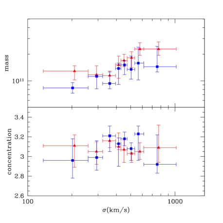
Figure 10: Median stellar mass (upper panel) and concentration (lower panel) for BCGs as function of the velocity dispersion of their host cluster. The red triangles and blue squares represent radio-loud and control radio-quiet BCGs, respectively. Horizontal error-bars show the range of the velocity dispersion bins, while vertical error-bars indicate the 32 to 68 percent ranges of the distributions.

Given that the radio-loud AGN are biased towards higher stellar mass galaxies, it is natural to ask whether the higher $L_{X}$ of our radio-loud clusters simply reflects the larger stellar masses of their BCGs. To investigate this issue, we first study the dependence of the $L_{X}-\sigma$ relation on BCG stellar mass, independent of BCG radio activity.

As before, we first divide our 625 clusters of galaxies into 8 velocity dispersion bins. We take the range of each bin to be the same as in Fig. 8. We then divide the clusters in each bin into three equal sub-samples according to the stellar mass of their BCGs. Combining velocity dispersion bins, gives us three sub-samples, which we refer to as the low, intermediate and high mass BCG samples. The median stellar mass of BCGs in these three samples are $7.76\times 10^{10}M_{\odot}$, $1.35\times 10^{11}M_{\odot}$ and $2.14\times 10^{11}M_{\odot}$. For comparison, the median stellar mass of the BCGs in our radio-loud and control radio-quiet cluster samples are $1.66\times 10^{11}M_{\odot}$ and $1.35\times 10^{11}M_{\odot}$, respectively. Thus, the high BCG mass sample has even larger median BCG mass than our radio-loud sample, while the low BCG mass sample has even lower median BCG mass than our control radio-quiet sample. The intermediate BCG mass sample have nearly the same median BCG mass as the control radio-quiet sample.

For each BCG mass sub-sample, we then combine all the clusters in each velocity dispersion bin into a single stack. For the low BCG mass sample, the X-ray detection of the velocity dispersion bin $\sigma>900\>{\rm km}\,{\rm s}^{-1}$ is not significant, so we combine all the clusters with $\sigma>800\>{\rm km}\,{\rm s}^{-1}$ into one stack, thus ending up with seven stacks for the low BCG mass sample and eight stacks for the intermediate and high BCG mass samples. We show the resulting $L_{X}-\sigma$ relations in the three panels of Fig. 11. As before, we use the BCSE orthogonal regression method to fit linear relations between $\,{\rm log}\,L_{X}$ and $\,{\rm log}\,\sigma$ weighted by the error on both $L_{X}$ and $\sigma$. The fitting relations are shown as solid lines each panel of Fig. 11, and the corresponding fitting parameters are listed in Table 1. The $L_{X}-\sigma$ relation for our stacks of radio-loud clusters [Equ. (11)] is shown as a dotted line in each panel for reference.

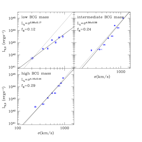
Figure 11: The $L_{X}-\sigma$ relation for stacks of clusters with high, intermediate and low BCG stellar masses (top left, top right and bottom left panels respectively). The solid lines in each panel show the best linear fits to the relation between $\,{\rm log}\,L_{X}$ and $\,{\rm log}\,\sigma$. The $L_{X}-\sigma$ relation for the stacks of radio-loud clusters [Equ. (11)] is shown as dotted line in each panel for comparison.

The X-ray luminosity of the clusters shows a very interesting dependence on the stellar mass of the BCGs. The high and intermediate BCG mass samples have have $L_{X}-\sigma$ relations which are both essentially identical to that of the radio-loud clusters. The low BCG mass sample, on the other hand, has an $L_{X}-\sigma$ relation which is significantly different. Clusters in the higher velocity dispersion bins are substantially less luminous than those in the other two samples. This results in a much shallower slope, $2.88\pm 0.17$, than the value $\sim 4$ found in all the other cases.

The fractions of radio-loud clusters are, as expected, higher in the samples with higher mass BCGs. The numbers for the low, intermediate and high mass samples are 12, 24 and 29 percent, respectively. We note that radio-loud fraction in the intermediate and high BCG mass samples do not differ very much, while the low BCG mass sample has significantly fewer radio-loud objects. Together, all these results imply that the stellar mass of BCGs is strongly coupled both with their radio activity and with the properties of the ICM. We now explore this connection further by examining the BCG stellar mass dependence of the $L_{X}-\sigma$ relation separately for radio-loud and radio-quiet clusters.

We split our radio-loud sample into two sub-samples with similar velocity dispersion and radio properties, but with systemically different BCG stellar masses. In detail, we separate the 134 radio-loud clusters into 67 pairs with very similar velocity dispersion and BCG radio luminosity. We then take the clusters with the higher BCG stellar mass in each pair to build the high BCG mass sub-sample, and the clusters with lower BCG stellar mass to build the low BCG mass sample. We split the 67 high BCG mass clusters into 6 velocity dispersion bins and make 6 stacks. Clusters with $\sigma$ in the range $300-600\>{\rm km}\,{\rm s}^{-1}$ are split into 3 equal bins with width $100\>{\rm km}\,{\rm s}^{-1}$; clusters with $600<\sigma<800\>{\rm km}\,{\rm s}^{-1}$ make up another stack. The remaining groups with $\sigma<300\>{\rm km}\,{\rm s}^{-1}$ and clusters with $\sigma>800\>{\rm km}\,{\rm s}^{-1}$ make up the two remaining stacks. For the low BCG mass sample, we make 6 corresponding stacks. For each pair of radio-loud clusters, if the high BCG mass object is binned into $j$th stack, the low BCG mass object is binned into $j$th stack also.

We also split the radio-quiet clusters into two sub-samples with differing BCG stellar mass. As for the whole sample, we first bin the clusters into 8 velocity dispersion bins. In each velocity dispersion bin, we then separate the clusters into equal low BCG mass and high BCG mass sub-samples. For each sub-sample, we combine all the clusters in each velocity dispersion bin into a single stack. For the low BCG mass sample, we combine the clusters in the two highest velocity dispersion bins ($800\>{\rm km}\,{\rm s}^{-1}<\sigma<900\>{\rm km}\,{\rm s}^{-1}$ and $\sigma>900\>{\rm km}\,{\rm s}^{-1}$), since the significance of the X-ray detection of the $\sigma>900\>{\rm km}\,{\rm s}^{-1}$ bin is too low.

We obtain significant X-ray detections for all stacks in these four samples. The resulting $L_{X}-\sigma$ relations are shown in figure 12. The two sub-samples of radio-loud clusters are shown in the top two panels, with the high BCG mass sample on the left and the low BCG mass sample on the right. The two radio-quiet sub-samples are shown in the same order in the bottom two panels. We use the BCSE orthogonal regression method to fit linear relations to the $\,{\rm log}\,L_{X}$ and $\,{\rm log}\,\sigma$ data in all these panels, weighting by the errors in both $L_{X}$ and $\sigma$. The fitting relations are shown as solid lines in each panel and the corresponding parameters are listed in Table 1. The $L_{X}-\sigma$ relation for the radio-loud stacks of the full sample [Equ. (11)] is again shown as a dotted line in each panel for reference.

Figure 12: The $L_{X}-\sigma$ relation for stacks of low BCG mass and high BCG mass sub-samples of radio-loud and radio-quiet clusters. The results for radio-loud and radio-quiet clusters are shown on the top and bottom rows, respectively. High BCG mass sub-samples are shown on the left and low BCG mass sub-samples on right. The solid lines in each panel show the best linear fits to the relations between $\,{\rm log}\,L_{X}$ and $\,{\rm log}\,\sigma$. The $L_{X}-\sigma$ relation for stacks of the full sample of radio-loud clusters [Equ. (11)] is shown as dotted line in each panel for reference.

Three of these four subsamples show very similar $L_{X}-\sigma$ relations, all of which are consistent with the relation for the full radio-loud sample. Only the radio-quiet subsample with low BCG mass shows a significantly different relation which in turn is very similar to that shown in Fig. 11 for the subsample with lowest BCG mass, independent of radio activity. Thus it seems that the $L_{X}-\sigma$ is similar for all clusters except those for which are both radio-quiet and have an unusually low mass BCG. Among radio-loud clusters we detect no dependence of the relation on BCG stellar mass. The difference between radio-loud and radio-quiet clusters appears to be due entirely to the presence of a subsample of relatively high velocity dispersion radio-quiet clusters which have both low BCG stellar mass and low X-ray luminosity. These might plausibly be systems which have not yet fully collapsed, so that both their X-ray luminosity and their BCG mass are typical of those usually found in lower mass relaxed systems.

To look more carefully for off-sets between our various subsamples we have refit the data plotted in Figs 11 and 12 fixing the slopes $a$ to be 2.97 for the low BCG mass and low BCG mass radio-quiet panels and 4.40 for the other five panels. The resulting zero-points $b^{\prime}$ are listed with their formal uncertainties in Table 1. The relations in each group are formally consistent within their errors, so we see no clear evidence justifying a more complex interpretation of the data. The most significant and suggestive difference is that the full radio-loud cluster sample is about 30% more X-ray luminous than the sample of high BCG mass radio-quiet clusters, even though the latter sample has a slightly larger median BCG mass. This result is significant at just over the $2\sigma$ level, suggesting that even at fixed cluster velocity dispersion and BCG mass, radio sources prefer to live in more X-ray luminous clusters.

6 Conclusions

We have used the ROSAT All Sky Survey to study the X-ray properties of a sample of 625 groups and clusters of galaxies selected from the Sloan Digital Sky Survey. We focus on the $L_{X}-\sigma$ relation of these groups and clusters, and we study whether this relation depends on the radio properties of the central galaxy (BCG). A cluster is termed ‘radio-loud’ if its central BCG is a radio-loud AGN, and ‘radio-quiet’ if the BCG is not detected at radio wavelengths. We find that the fraction of clusters with individual X-ray detections depends strongly on whether the BCG is radio-loud. Radio-loud clusters are detected more frequently than radio-quiet clusters of the same velocity dispersion and redshift.

The $L_{X}-\sigma$ relations for individually detected radio-loud and radio-quiet clusters are very similar, but this is purely a selection bias. The majority of detected clusters are just above the X-ray detection limit in both samples. Since the redshift distribution at each velocity dispersion is similar for the two types of cluster, the mean relations for detected objects are forced to be similar.

By stacking the X-ray images of clusters with similar velocity dispersion, we studied the average X-ray luminosities and surface brightness profiles of our clusters as function of velocity dispersion. The average X-ray luminosities of radio-loud clusters are systematically higher and their luminosity profiles are more concentrated than those of radio-quiet systems. X-ray emission from the radio AGN itself is by far insufficient to explain this doubling of the X-ray luminosity. Our results demonstrate convincingly and quantitatively that the X-ray properties of the intracluster gas correlate with the presence of a central radio source in the way first suggested by Burns (1990).

The stellar masses of the BCGs also correlate with their radio properties; radio-loud clusters tend to mave more massive BCGs than radio-quiet clusters of the same velocity dispersion. Those clusters of given velocity dispersion which have unusually low mass BCGs tend to be both underluminous in X-rays and radio-quiet. This effect is particularly pronounced for large velocity dispersion clusters. Among radio-loud clusters we find no dependence of X-ray luminosity on BCG stellar mass. These results can be summarised by saying that the only clear dependence of X-ray properties on BCG properties is that high velocity dispersion clusters in which the BCG is both low mass and radio-quiet tend to be several times less X-ray luminous than otherwise similar clusters in which the BCG is massive and/or radio-loud.

Clearly a high central hot gas density is needed for effective fuelling of the radio source. If the radio activity is in turn able to heat the surrounding gas and cause its re-expansion, the feedback cycle needed to control the growth of the central galaxy could be established. The conditions which lead to effective AGN fuelling are clearly related to the presence of a massive central galaxy, although the exact causal relationship between BCG growth, AGN activity and ICM structure remains to be clarified.

Appendix A The clusters of galaxies individually detected in RASS

Here we list the basic properties of 142 clusters of galaxies individually detected in RASS. The description of the columns is as follows.

• column 1: the ID of cluster in SDSS C4 cluster catalogue(http://www.ctio.noao.edu/ chrism/C4/)

• column 2: the Right Ascension(J2000) of the BCG in decimal degrees

• column 3: the Declination(J2000) of the BCG in decimal degrees

• column 4: the Right Ascension(J2000) of the X-ray centre in decimal degrees

• column 5: the Declination(J2000) of the X-ray centre in decimal degrees

• column 6: the redshift of the BCG

• column 7: the virial radius $R_{200}$ in unit of arcmin

• column 8: the velocity dispersion in unit of $\>{\rm km}\,{\rm s}^{-1}$

• column 9: the flux within $R_{X}$ in the energy band 0.5-2.0kev, in unit of $10^{-12}$ erg $\rm{s}^{-1}\rm{cm}^{-2}$

• column 10: the X-ray extension radius $R_{X}$, in unit of arcmin

• column 11: the fractional error on count rate(flux) within $R_{X}$

• column 12: the extension correction factor $f_{E}$[equation (4)]

• column 13: the bolometric X-ray luminosity after the extension, in unit of $10^{44}$ erg $\rm{s}^{-1}$

• column 14: the classification of radio properties of BCG, 1 for the clusters with BCG to be radio-loud AGN, 0 for the clusters with BCG to be radio-quiet, $-1$ for others

ID	RA	Dec	$\rm{RA_{X}}$	$\rm{Dec_{X}}$	$z$	$R_{200}$	$\sigma$	$f_{X}$	$R_{X}$	Err	$f_{E}$	$L_{44}$	R-class
(1)	(2)	(3)	(4)	(5)	(6)	(7)	(8)	(9)	(10)	(11)	(12)	(13)	(14)
1000	202.54301	-2.10501	$-$	$-$	0.0867	14.2	647.8	1.553	7.0	0.308	1.186	0.529	1
1048	205.54018	2.22721	205.5251	2.2276	0.0774	20.5	827.5	5.339	9.0	0.147	1.324	1.950	0
1066	202.79596	-1.72731	202.8011	-1.7162	0.0854	18.2	814.2	6.297	18.0	0.218	1.002	2.102	0
1001	208.27667	5.14974	208.3057	5.2152	0.0794	18.0	746.4	6.316	11.0	0.116	1.146	1.924	0
1002	159.77759	5.20977	$-$	$-$	0.0690	22.3	800.4	4.222	10.0	0.241	1.311	1.168	0
1004	184.42136	3.65581	184.4206	3.6600	0.0774	23.9	966.0	19.892	14.0	0.055	1.165	7.462	0
1017	182.57005	5.38603	182.5764	5.3857	0.0769	14.8	596.0	5.263	10.0	0.111	1.109	1.242	0
1069	184.71817	5.24567	$-$	$-$	0.0764	18.1	721.3	1.161	8.0	0.323	1.320	0.365	0
1087	183.73737	5.04247	183.7515	5.0156	0.0782	11.4	465.0	2.945	7.0	0.135	1.144	0.684	0
1212	148.42239	1.70070	148.4196	1.7052	0.0977	7.5	388.3	1.424	6.0	0.189	1.042	0.459	1
1006	191.30367	1.80480	$-$	$-$	0.0477	13.9	340.3	1.950	10.0	0.327	1.085	0.135	0
1044	194.67288	-1.76146	194.6711	-1.7589	0.0837	17.6	771.0	19.671	10.0	0.061	1.178	7.064	0
1058	195.71906	-2.51635	195.7177	-2.5096	0.0831	17.2	748.7	3.737	7.0	0.160	1.381	1.511	0
1016	175.29919	5.73480	175.2950	5.7151	0.0983	12.7	660.1	0.799	5.0	0.325	1.296	0.391	1
1041	179.37073	5.08906	$-$	$-$	0.0758	17.1	678.2	2.836	9.0	0.176	1.217	0.774	0
1011	198.05661	-0.97449	198.0540	-0.9832	0.0847	14.2	631.4	1.115	5.0	0.328	1.511	0.453	0
1028	199.13568	0.87025	199.1394	0.8830	0.0796	8.7	363.5	0.525	3.0	0.331	1.535	0.156	0
1047	197.32954	-1.62253	197.3326	-1.6232	0.0829	12.0	521.1	3.234	9.0	0.197	1.055	0.803	1
1189	201.57338	0.22150	201.5723	0.2214	0.0829	11.9	516.6	5.114	7.0	0.122	1.163	1.394	0
1372	201.76564	1.33573	201.7738	1.3475	0.0804	16.1	677.4	1.569	9.0	0.298	1.186	0.471	0
1013	227.10735	-0.26629	227.1060	-0.2585	0.0906	15.7	747.9	0.830	4.0	0.327	1.944	0.564	0
1151	226.68803	-1.23171	226.6998	-1.2309	0.0710	13.5	500.4	1.928	10.0	0.308	1.078	0.349	0
1355	227.88237	1.76388	227.8839	1.7574	0.0390	19.6	391.7	2.039	11.0	0.261	1.184	0.105	0
1014	220.17848	3.46542	220.1600	3.4738	0.0269	33.4	459.0	10.640	14.0	0.092	1.359	0.317	0
1025	153.40948	-0.92541	153.4424	-0.8592	0.0451	34.0	789.8	8.720	13.0	0.092	1.434	1.085	0
1075	153.43707	-0.12022	153.4424	-0.1068	0.0944	17.6	875.5	3.496	10.0	0.163	1.178	1.814	0
1167	154.45268	-0.03077	154.4389	-0.0330	0.0638	12.2	405.9	0.732	5.0	0.296	1.379	0.130	0
1020	214.39804	2.05322	$-$	$-$	0.0540	21.7	605.2	2.546	13.0	0.248	1.115	0.292	1
1200	216.19754	2.66442	216.1944	2.6688	0.0543	21.1	592.4	1.911	8.0	0.232	1.318	0.259	1
1032	218.49640	3.77800	$-$	$-$	0.0290	38.4	569.8	2.471	13.0	0.260	1.552	0.107	0
1039	186.87810	8.82456	186.8716	8.8272	0.0897	17.9	846.1	3.487	9.0	0.160	1.243	1.655	0
1042	228.80879	4.38621	228.8193	4.3951	0.0980	16.6	856.8	3.443	8.0	0.183	1.194	1.914	1
1351	228.79631	3.84851	228.7980	3.8472	0.0786	11.4	468.1	1.327	5.0	0.243	1.237	0.337	1
1043	168.33385	2.54667	168.3346	2.5354	0.0743	10.4	403.5	4.700	12.0	0.132	0.973	0.807	0
1142	164.54578	1.60458	164.5436	1.5880	0.0394	21.3	430.1	3.131	14.0	0.189	1.118	0.162	0
1138	190.67690	2.78430	$-$	$-$	0.0858	6.9	308.9	3.400	9.0	0.325	0.952	0.707	0
1088	157.09782	3.75874	157.0948	3.7690	0.0735	15.4	591.3	1.798	5.0	0.218	1.427	0.494	1
1079	170.38568	2.88726	170.4047	2.8885	0.0494	22.6	576.4	4.866	12.0	0.135	1.212	0.492	0
1101	140.65239	-0.40903	$-$	$-$	0.0557	15.0	431.8	1.246	11.0	0.316	1.060	0.127	1
1109	170.72636	1.11440	170.7152	1.0901	0.0742	13.8	535.5	1.251	6.0	0.259	1.243	0.293	1
1118	181.11276	1.89600	181.1214	1.9107	0.0202	49.0	501.9	17.039	19.0	0.068	1.421	0.303	0
1166	165.18890	10.55318	165.2048	10.5490	0.0355	41.4	754.2	4.677	15.0	0.167	1.483	0.354	0
1247	165.23923	10.50548	165.2048	10.5490	0.0354	39.3	713.2	4.345	15.0	0.181	1.314	0.277	1
1283	125.74545	4.29911	125.7623	4.3040	0.0954	15.0	754.3	6.416	14.0	0.174	1.015	2.555	0
1356	125.84028	4.37247	125.8387	4.3769	0.0300	31.6	483.7	6.961	20.0	0.193	1.098	0.213	1
2001	351.08368	14.64713	351.0534	14.6617	0.0417	32.4	694.8	11.503	12.0	0.079	1.463	1.114	-1
2002	358.55701	-10.41920	358.5537	-10.4070	0.0762	20.4	811.8	8.252	8.0	0.098	1.298	2.809	1
2127	358.77844	-9.37558	358.7696	-9.3906	0.0746	8.3	323.5	0.720	5.0	0.317	1.153	0.135	0
2004	329.37259	-7.79571	329.3703	-7.7822	0.0579	20.9	626.6	3.805	12.0	0.216	1.174	0.542	0
2005	18.24821	15.49129	18.2552	15.5148	0.0433	22.7	506.5	4.214	11.0	0.163	1.264	0.319	-1
2013	10.46027	-9.30315	10.4438	-9.2373	0.0556	31.4	903.2	67.080	19.0	0.032	1.112	11.316	1
2015	29.07064	1.05083	$-$	$-$	0.0797	17.8	742.2	1.107	9.0	0.322	1.238	0.365	0
2031	30.57201	-1.12784	30.5779	-1.1174	0.0426	13.2	289.2	1.959	9.0	0.192	1.105	0.110	-1
2016	18.73999	0.43080	$-$	$-$	0.0449	23.9	552.1	7.170	15.0	0.114	1.136	0.544	0
2141	20.09640	-0.07920	20.0900	-0.0822	0.0779	10.4	421.6	0.557	4.0	0.301	1.306	0.144	1
2020	328.52530	-8.64287	328.5050	-8.6421	0.0740	13.1	504.9	1.689	6.0	0.247	1.296	0.403	0
2026	14.06715	-1.25537	14.1457	-1.2683	0.0444	40.9	933.0	36.308	29.0	0.058	1.091	3.914	0
2032	7.36845	-0.21261	7.3811	-0.2333	0.0597	14.8	458.1	1.035	9.0	0.315	1.149	0.136	0
2081	5.63777	-0.92657	$-$	$-$	0.0580	7.1	214.4	0.609	5.0	0.290	1.095	0.081	0
2054	22.88717	0.55597	22.9058	0.5454	0.0794	12.4	513.7	1.817	8.0	0.196	1.092	0.425	1
2030	333.69534	13.84087	333.7197	13.8406	0.0260	30.2	400.2	2.865	10.0	0.184	1.575	0.087	-1
2036	337.29065	0.07890	337.2749	0.0816	0.0578	12.7	381.0	1.230	6.0	0.307	1.205	0.147	1
2047	24.31406	-9.19761	24.3182	-9.1959	0.0406	21.9	455.4	6.109	10.0	0.090	1.218	0.374	1
2049	334.06497	-9.33325	334.0629	-9.3436	0.0841	12.6	555.0	7.479	6.0	0.113	1.199	2.222	1
2125	334.41815	-9.19784	334.4119	-9.2061	0.0945	3.8	189.4	0.957	5.0	0.299	0.952	0.346	0
2050	17.51319	13.97812	17.5271	14.0028	0.0588	24.9	759.2	1.186	6.0	0.251	2.050	0.352	-1
2069	16.84109	14.27322	16.8257	14.2764	0.0746	18.5	720.4	1.002	7.0	0.311	1.442	0.328	-1
2112	315.59933	0.25743	315.6010	0.2616	0.0510	8.0	211.7	1.107	5.0	0.210	1.140	0.119	-1
3280	133.67439	40.40579	133.6850	40.4256	0.0877	8.3	381.9	0.764	6.0	0.309	1.084	0.202	0
3074	225.28316	47.27660	225.2898	47.2864	0.0880	15.2	704.6	3.120	9.0	0.135	1.161	1.136	0
3325	230.12077	44.97098	230.1225	44.9753	0.0639	14.3	472.8	0.677	6.0	0.261	1.259	0.114	1
3002	255.63808	33.51668	255.6381	33.5032	0.0880	20.6	951.1	2.036	9.0	0.162	1.239	1.042	1
3012	255.67708	34.06002	255.5988	34.1199	0.0990	21.5	1126.7	19.775	16.0	0.043	1.076	13.537	0
3059	257.45279	34.45899	257.4865	34.4483	0.0858	11.8	529.9	10.775	12.0	0.062	0.996	2.728	0
3003	177.02458	54.64628	$-$	$-$	0.0597	17.3	534.9	2.385	11.0	0.211	1.130	0.322	0
3018	176.83920	55.73010	176.8489	55.7536	0.0517	25.6	683.7	3.823	14.0	0.160	1.197	0.467	0
3065	180.05794	56.25068	180.0793	56.2321	0.0649	21.5	723.8	3.809	13.0	0.175	1.112	0.723	1
3004	258.12006	64.06076	257.9521	64.0853	0.0801	27.6	1155.8	21.210	31.0	0.033	0.977	8.750	0
3060	259.62976	64.41811	259.6574	64.4133	0.0895	8.4	393.4	0.540	11.0	0.217	0.952	0.133	-1
3186	258.87518	64.66431	258.7888	64.6897	0.0795	9.8	409.2	0.568	9.0	0.162	1.020	0.118	-1
3599	255.49088	59.58125	$-$	$-$	0.0872	15.1	691.2	0.574	7.0	0.313	1.212	0.211	1
3005	239.58334	27.23342	239.5733	27.2463	0.0901	20.6	974.1	53.559	14.0	0.030	1.105	26.333	0
3096	152.56697	54.50182	152.5529	54.4864	0.0460	16.5	389.8	1.180	9.0	0.236	1.197	0.087	-1
3009	140.20340	40.66420	$-$	$-$	0.0740	12.4	480.6	1.003	7.0	0.303	1.184	0.216	0
3011	182.19380	53.33370	182.2094	53.3377	0.0820	12.2	524.1	0.990	5.0	0.253	1.377	0.314	0
3014	187.19733	51.26526	187.1927	51.2717	0.0858	9.1	408.5	0.643	4.0	0.263	1.235	0.191	1
3033	174.01463	55.07530	$-$	$-$	0.0564	15.1	440.6	1.184	9.0	0.270	1.157	0.137	0
3043	168.84946	54.44410	168.8787	54.4444	0.0698	17.1	621.4	2.282	8.0	0.155	1.208	0.491	1
3097	173.09666	55.96744	173.0826	55.9802	0.0514	13.7	364.4	3.027	8.0	0.134	1.168	0.269	0
3159	174.78577	55.66448	174.8184	55.6735	0.0611	13.9	439.7	0.692	6.0	0.305	1.244	0.102	1
3016	127.13190	30.43130	127.2076	30.4518	0.0498	32.0	821.5	7.418	14.0	0.107	1.329	1.084	0
3020	156.25665	47.84185	156.2658	47.8105	0.0629	18.8	613.0	1.977	9.0	0.176	1.269	0.357	0
3140	151.31216	53.14899	$-$	$-$	0.0449	27.6	637.4	1.120	8.0	0.261	1.741	0.141	0
3577	158.16068	53.15659	$-$	$-$	0.0637	12.0	397.4	0.856	10.0	0.321	1.043	0.113	0
3023	163.40237	54.86794	163.4248	54.9388	0.0719	14.9	556.4	3.177	8.0	0.121	1.205	0.684	0
3115	158.24541	56.74816	158.2825	56.7529	0.0451	18.4	426.5	0.432	5.0	0.330	1.588	0.042	1
3120	160.25429	58.29495	160.2388	58.2836	0.0732	11.7	444.8	1.230	5.0	0.176	1.342	0.289	0
3167	162.30042	57.83725	$-$	$-$	0.0732	13.8	525.5	0.735	4.0	0.268	1.737	0.233	0
3171	163.34550	56.31446	163.3528	56.3233	0.0765	10.5	418.0	0.496	5.0	0.300	1.270	0.120	0
3205	164.94170	53.80363	164.9784	53.8232	0.0723	11.3	426.9	0.635	5.0	0.260	1.322	0.142	0
3025	173.70541	49.07763	$-$	$-$	0.0330	39.1	661.2	6.992	16.0	0.131	1.274	0.354	1
3408	168.92094	48.57265	$-$	$-$	0.0740	9.4	362.7	0.796	9.0	0.319	1.007	0.133	1
3026	136.97687	52.79053	136.9746	52.7910	0.0979	11.3	583.1	1.121	7.0	0.306	1.105	0.431	1
3100	136.98473	49.59673	136.9897	49.5927	0.0352	24.1	434.2	1.888	7.0	0.187	1.522	0.107	1
3027	230.21770	48.66073	230.2238	48.6683	0.0737	17.4	669.8	5.709	8.0	0.093	1.216	1.455	1
3041	229.99155	51.31306	229.9925	51.3328	0.0776	13.7	555.0	0.484	6.0	0.322	1.238	0.125	1
3050	232.31100	52.86400	232.3134	52.8470	0.0734	16.6	635.1	1.973	9.0	0.141	1.201	0.475	0
3028	204.03470	59.20640	204.0723	59.2271	0.0704	23.8	872.3	12.147	13.0	0.057	1.197	3.470	0
3114	203.26436	60.11770	203.2779	60.1178	0.0719	13.4	502.7	1.659	9.0	0.164	1.083	0.310	1
3029	183.70267	59.90620	183.7677	59.9160	0.0599	14.1	436.8	1.303	10.0	0.251	1.090	0.161	0
3031	247.15930	39.55122	247.3164	39.5735	0.0305	48.4	754.6	95.497	29.0	0.020	1.115	3.984	1
3051	247.43703	40.81166	247.4344	40.8138	0.0304	38.5	596.9	6.874	21.0	0.106	1.146	0.247	1
3182	244.50175	41.39219	244.5108	41.3899	0.0614	11.0	351.8	0.795	5.0	0.210	1.305	0.114	0
3326	245.76302	37.92238	245.7615	37.9223	0.0312	38.1	608.5	2.444	10.0	0.142	1.627	0.133	1
3583	242.80766	36.97338	242.8176	36.9768	0.0673	14.6	512.2	0.855	5.0	0.263	1.387	0.180	1
3084	118.36082	29.35946	118.3380	29.3811	0.0607	24.8	781.3	6.563	10.0	0.100	1.390	1.443	0
3094	254.93312	32.61532	254.9353	32.6184	0.0976	17.0	874.8	4.491	8.0	0.088	1.204	2.549	1
3038	191.85095	54.98703	$-$	$-$	0.0833	14.3	625.3	1.308	10.0	0.282	1.097	0.370	0
3163	146.70914	43.42387	$-$	$-$	0.0725	8.3	314.9	0.490	5.0	0.331	1.114	0.084	1
3422	195.66270	62.49424	195.6442	62.5186	0.0765	7.8	310.2	0.592	6.0	0.280	1.048	0.106	1
3071	122.41201	34.92701	122.4113	34.9286	0.0824	9.2	398.3	3.746	7.0	0.144	1.052	0.859	1
3176	122.53550	35.27528	122.5413	35.2943	0.0841	14.2	626.8	1.310	5.0	0.287	1.511	0.523	0
3055	116.67855	30.99707	116.6630	30.9956	0.0581	22.5	675.1	1.182	5.0	0.272	2.216	0.336	0
3057	242.40390	53.04123	242.4066	53.0429	0.0631	14.3	467.9	1.608	9.0	0.175	1.134	0.237	0
3195	242.03407	49.20098	242.0678	49.2017	0.0598	6.7	206.4	0.429	4.0	0.289	1.114	0.064	1
3088	146.68938	54.42693	146.6944	54.4797	0.0463	23.3	555.7	3.576	10.0	0.152	1.249	0.319	1
3357	140.86415	54.82936	140.8650	54.8234	0.0457	19.7	462.3	1.121	9.0	0.278	1.218	0.088	1
3069	168.79204	61.11019	$-$	$-$	0.0554	15.4	441.3	0.830	9.0	0.281	1.166	0.093	0
3079	254.08789	39.27516	254.0892	39.2780	0.0622	13.5	436.0	1.642	8.0	0.179	1.160	0.234	0
3083	212.95599	52.81670	212.9562	52.8180	0.0760	11.8	470.1	0.799	7.0	0.249	1.119	0.171	1
3155	213.97035	50.32380	213.9704	50.3376	0.0745	12.6	488.6	0.647	5.0	0.268	1.400	0.167	0
3430	212.04359	52.68005	212.0370	52.6660	0.0819	5.3	225.9	0.380	4.0	0.279	1.052	0.094	1
3091	244.33394	34.90165	244.3308	34.9082	0.0309	32.6	514.8	5.982	14.0	0.089	1.341	0.242	-1
3092	129.04651	38.53475	129.0240	38.5458	0.0568	15.2	447.6	1.365	7.0	0.216	1.295	0.180	0
3247	126.50238	40.98111	$-$	$-$	0.0571	10.4	306.6	0.677	5.0	0.262	1.195	0.074	1
3103	243.49199	49.18961	$-$	$-$	0.0577	17.0	507.4	0.848	6.0	0.296	1.507	0.139	0
3113	212.51746	41.75580	212.5277	41.7565	0.0936	11.6	572.5	0.833	5.0	0.266	1.339	0.350	0
3122	122.59694	42.27387	122.5905	42.2771	0.0638	15.1	501.0	2.867	8.0	0.153	1.158	0.446	1
3131	217.08293	45.98601	$-$	$-$	0.0749	7.5	294.7	0.576	8.0	0.329	0.991	0.094	1
3271	215.39972	44.70806	215.4122	44.7125	0.0915	8.1	388.9	0.499	5.0	0.293	1.141	0.153	0
3389	217.45209	53.96503	217.4551	53.9706	0.0429	15.0	332.2	0.434	4.0	0.255	1.873	0.041	0
3143	261.86160	58.51655	$-$	$-$	0.0279	32.9	469.2	0.409	6.0	0.246	2.769	0.027	0
3152	258.84579	57.41119	258.7895	57.4464	0.0293	38.9	582.5	13.278	16.0	0.041	1.271	0.484	1
3375	260.85498	56.97455	260.8525	56.9782	0.0282	36.4	525.0	2.289	11.0	0.115	1.685	0.098	-1
3249	118.93488	41.20394	118.9279	41.2039	0.0740	14.0	541.4	1.115	6.0	0.263	1.344	0.282	0
3149	159.30116	50.12058	159.2658	50.0983	0.0451	20.1	466.5	1.549	10.0	0.216	1.248	0.122	-1
3157	138.28223	47.70844	138.2839	47.7101	0.0513	13.8	366.1	1.933	8.0	0.205	1.126	0.166	1
3166	238.75801	41.57834	$-$	$-$	0.0340	35.8	623.0	1.640	10.0	0.283	1.793	0.119	0
3168	131.08771	51.40593	131.0757	51.4143	0.0971	7.9	405.9	0.402	3.0	0.324	1.318	0.165	1
3173	186.12561	66.56688	186.1431	66.5724	0.0870	9.5	432.4	0.438	5.0	0.328	1.215	0.133	-1
3196	244.63882	43.08144	244.6446	43.0932	0.0603	16.4	511.9	0.508	4.0	0.333	2.023	0.123	0
3222	246.85513	42.67971	246.8527	42.6750	0.0313	17.0	271.5	2.122	12.0	0.137	1.092	0.064	0
3208	170.56416	67.22186	170.5571	67.2284	0.0552	9.3	264.5	0.778	5.0	0.192	1.203	0.085	-1
3212	117.48110	29.42018	$-$	$-$	0.0631	12.0	392.4	0.529	5.0	0.325	1.363	0.089	0
3283	135.32254	58.27975	135.3272	58.2702	0.0977	14.7	755.9	1.181	7.0	0.251	1.271	0.621	0
3516	263.05081	59.94155	263.0525	59.9425	0.0290	9.7	143.6	0.254	4.0	0.215	1.372	0.013	0
3315	258.62753	65.28972	258.6241	65.2898	0.0799	9.5	396.0	0.372	7.0	0.182	1.078	0.082	-1
3349	251.93350	29.94190	$-$	$-$	0.0996	16.8	883.6	4.197	7.0	0.114	1.363	2.843	0
3425	261.37708	53.02419	$-$	$-$	0.0612	12.6	398.8	0.636	8.0	0.235	1.097	0.080	1

Appendix B Examples of our procedure for detecting clusters in the RASS

In the following, we show two example images where decisions about the X-ray detections had to be made by eye. The first example deals with the process of determining of the X-ray centre of the cluster (Section 3.1). Some X-ray sources, which are although inside the 5 arcmin aperture of the BCGs, are judged as contaminating sources rather than the X-ray centres of the clusters (Fig. B1). The second example deals with the procedure of distinguishing contaminating X-ray sources from the extended X-ray emission of the cluster (Fig. B2).

Figure 13: The RASS image of the C4 cluster 1094. The cross shows the position of the BCG and the big circle enclosed the region of the cluster within a distance $R_{200}$($\sim$ 8 arcimin) from the cluster centre. The small circle shows the X-ray point source detected near the cluster centre. The angular distance from the X-ray source to the position of the BCG is $\sim$3 arcmin. This X-ray source is judged to be a contaminant and not associated with the X-ray emission of the cluster.

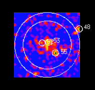
Figure 14: The RASS image of the C4 cluster 1049. The cross shows the position of the BCG and the small circles show the ML detected X-ray sources. The inner big circle shows the region within a distance $R_{200}$ ($\sim$ 16.5 arcimin) from the cluster centre, while the outer circle has a radius of $R_{200}+6$ arcmin. The area inside the ring from $R_{200}$ to $R_{200}+6$ arcmin is used for the background estimation. In this image, sources 48 and 55 are considered as contaminants, while sources 52 and 53 are considered as part of the extended X-ray emission from the cluster.

References

- Akritas & Bershady (1996) Akritas M. G., Bershady M. A., 1996, ApJ, 470, 706
- Allen et al. (2006) Allen S. W., Dunn R. J. H., Fabian A. C., Taylor G. B., Reynolds C. S., 2006, MNRAS, 372, 21
- Bartelmann & White (2003) Bartelmann M., White S. D. M., 2003, A&A, 407, 845
- Bautz & Morgan (1970) Bautz L. P., Morgan W. W., 1970, ApJL, 162, L149+
- Becker et al. (1995) Becker R. H., White R. L., Helfand D. J., 1995, ApJ, 450, 559
- Best et al. (2005) Best P. N., Kauffmann G., Heckman T. M., Brinchmann J., Charlot S., Ivezić Ž., White S. D. M., 2005, MNRAS, 362, 25
- Best et al. (2007) Best P. N., von der Linden A., Kauffmann G., Heckman T. M., Kaiser C. R., 2007, MNRAS, 379, 894
- Blanton et al. (2003) Blanton E. L., Sarazin C. L., McNamara B. R., 2003, ApJ, 585, 227
- Boehringer et al. (1993) Boehringer H., Voges W., Fabian A. C., Edge A. C., Neumann D. M., 1993, MNRAS, 264, L25
- Böhringer et al. (2004) Böhringer H., Schuecker P., Guzzo L., Collins C. A., Voges W., Cruddace R. G., Ortiz-Gil A., Chincarini G., De Grandi S., Edge A. C., MacGillivray H. T., Neumann D. M., Schindler S., Shaver P., 2004, A&A, 425, 367
- Böhringer et al. (2000) Böhringer H., Voges W., Huchra J. P., McLean B., Giacconi R., Rosati P., Burg R., Mader J., Schuecker P., Simiç D., Komossa S., Reiprich T. H., Retzlaff J., Trümper J., 2000, ApJS, 129, 435
- Bower et al. (2006) Bower R. G., Benson A. J., Malbon R., Helly J. C., Frenk C. S., Baugh C. M., Cole S., Lacey C. G., 2006, MNRAS, 370, 645
- Brinkmann et al. (2000) Brinkmann W., Laurent-Muehleisen S. A., Voges W., Siebert J., Becker R. H., Brotherton M. S., White R. L., Gregg M. D., 2000, A&A, 356, 445
- Burns (1990) Burns J. O., 1990, AJ, 99, 14
- Chen et al. (2007) Chen Y., Reiprich T. H., Böhringer H., Ikebe Y., Zhang Y.-Y., 2007, A&A, 466, 805
- Churazov et al. (2000) Churazov E., Forman W., Jones C., Böhringer H., 2000, A&A, 356, 788
- Churazov et al. (2005) Churazov E., Sazonov S., Sunyaev R., Forman W., Jones C., Böhringer H., 2005, MNRAS, 363, L91
- Clarke et al. (2005) Clarke T. E., Sarazin C. L., Blanton E. L., Neumann D. M., Kassim N. E., 2005, ApJ, 625, 748
- Condon et al. (1998) Condon J. J., Cotton W. D., Greisen E. W., Yin Q. F., Perley R. A., Taylor G. B., Broderick J. J., 1998, AJ, 115, 1693
- Croston et al. (2005) Croston J. H., Hardcastle M. J., Birkinshaw M., 2005, MNRAS, 357, 279
- Croton et al. (2006) Croton D. J., Springel V., White S. D. M., De Lucia G., Frenk C. S., Gao L., Jenkins A., Kauffmann G., Navarro J. F., Yoshida N., 2006, MNRAS, 365, 11
- Dai et al. (2007) Dai X., Kochanek C. S., Morgan N. D., 2007, ApJ, 658, 917
- David et al. (1999) David L. P., Forman W., Jones C., 1999, ApJ, 519, 533
- Dickey & Lockman (1990) Dickey J. M., Lockman F. J., 1990, ARA&A, 28, 215
- Edge & Stewart (1991) Edge A. C., Stewart G. C., 1991, MNRAS, 252, 428
- Ettori et al. (2002) Ettori S., Fabian A. C., Allen S. W., Johnstone R. M., 2002, MNRAS, 331, 635
- Fabian (1994) Fabian A. C., 1994, ARA&A, 32, 277
- Fabian et al. (1994) Fabian A. C., Crawford C. S., Edge A. C., Mushotzky R. F., 1994, MNRAS, 267, 779
- Fabian et al. (2000) Fabian A. C., Sanders J. S., Ettori S., Taylor G. B., Allen S. W., Crawford C. S., Iwasawa K., Johnstone R. M., Ogle P. M., 2000, MNRAS, 318, L65
- Girardi et al. (1996) Girardi M., Fadda D., Giuricin G., Mardirossian F., Mezzetti M., Biviano A., 1996, ApJ, 457, 61
- Gitti et al. (2007) Gitti M., McNamara B. R., Nulsen P. E. J., Wise M. W., 2007, ApJ, 660, 1118
- Jetha et al. (2008) Jetha N. N., Hardcastle M. J., Babul A., O’Sullivan E., Ponman T. J., Raychaudhury S., Vrtilek J., 2008, MNRAS, 384, 1344
- Jetha et al. (2007) Jetha N. N., Ponman T. J., Hardcastle M. J., Croston J. H., 2007, MNRAS, 376, 193
- Kang et al. (2006) Kang X., Jing Y. P., Silk J., 2006, ApJ, 648, 820
- Katayama et al. (2003) Katayama H., Hayashida K., Takahara F., Fujita Y., 2003, ApJ, 585, 687
- Koester et al. (2007) Koester B. P., McKay T. A., Annis J., Wechsler R. H., Evrard A., Bleem L., Becker M., Johnston D., Sheldon E., Nichol R., Miller C., Scranton R., Bahcall N., Barentine J., Brewington H., 2007, ApJ, 660, 239
- Ledlow et al. (2003) Ledlow M. J., Voges W., Owen F. N., Burns J. O., 2003, AJ, 126, 2740
- McNamara et al. (2000) McNamara B. R., Wise M., Nulsen P. E. J., David L. P., Sarazin C. L., Bautz M., Markevitch M., Vikhlinin A., Forman W. R., Jones C., Harris D. E., 2000, ApJL, 534, L135
- Merloni et al. (2003) Merloni A., Heinz S., di Matteo T., 2003, MNRAS, 345, 1057
- Miller et al. (2005) Miller C. J., Nichol R. C., Reichart D., Wechsler R. H., Evrard A. E., Annis J., McKay T. A., Bahcall N. A., Bernardi M., Boehringer H., Connolly A. J., Goto T., Kniazev A., Lamb D., Postman M., Schneider D. P., Sheth R. K., Voges W., 2005, AJ, 130, 968
- Mulchaey (2000) Mulchaey J. S., 2000, ARA&A, 38, 289
- Nath & Roychowdhury (2002) Nath B. B., Roychowdhury S., 2002, MNRAS, 333, 145
- Neumann & Arnaud (1999) Neumann D. M., Arnaud M., 1999, A&A, 348, 711
- Nusser & Silk (2008) Nusser A., Silk J., 2008, MNRAS, pp 420–+
- O’Hara et al. (2006) O’Hara T. B., Mohr J. J., Bialek J. J., Evrard A. E., 2006, ApJ, 639, 64
- Omma & Binney (2004) Omma H., Binney J., 2004, MNRAS, 350, L13
- Ortiz-Gil et al. (2004) Ortiz-Gil A., Guzzo L., Schuecker P., Böhringer H., Collins C. A., 2004, MNRAS, 348, 325
- Peres et al. (1998) Peres C. B., Fabian A. C., Edge A. C., Allen S. W., Johnstone R. M., White D. A., 1998, MNRAS, 298, 416
- Raymond & Smith (1977) Raymond J. C., Smith B. W., 1977, ApJS, 35, 419
- Rizza et al. (2000) Rizza E., Loken C., Bliton M., Roettiger K., Burns J. O., Owen F. N., 2000, AJ, 119, 21
- Rykoff et al. (2008) Rykoff E. S., McKay T. A., Becker M. R., Evrard A., Johnston D. E., Koester B. P., Rozo E., Sheldon E. S., Wechsler R. H., 2008, ApJ, 675, 1106
- Shen et al. (2006) Shen S., White S. D. M., Mo H. J., Voges W., Kauffmann G., Tremonti C., Anderson S. F., 2006, MNRAS, 369, 1639
- Shimasaku et al. (2001) Shimasaku K., Fukugita M., Doi M., Hamabe M., Ichikawa T., Okamura S., Sekiguchi M., Yasuda N., Brinkmann J., Csabai I., Ichikawa S.-I., Ivezić Z., Kunszt P. Z., Schneider D. P., Szokoly G. P., Watanabe M., York D. G., 2001, AJ, 122, 1238
- Tremaine et al. (2002) Tremaine S., Gebhardt K., Bender R., Bower G., Dressler A., Faber S. M., Filippenko A. V., Green R., Grillmair C., Ho L. C., Kormendy J., Lauer T. R., Magorrian J., Pinkney J., Richstone D., 2002, ApJ, 574, 740
- Voges et al. (1999) Voges W., Aschenbach B., Boller T., Bräuninger H., Briel U., Burkert W., Dennerl K., Englhauser J., Gruber R., Haberl F., Hartner G., Hasinger G., 1999, A&A, 349, 389
- Voges et al. (2000) Voges W., Aschenbach B., Boller T., Brauninger H., Briel U., Burkert W., Dennerl K., Englhauser J., Gruber R., Haberl F., Hartner G., Hasinger G., 2000, IAUC, 7432, 3
- von der Linden et al. (2007) von der Linden A., Best P. N., Kauffmann G., White S. D. M., 2007, MNRAS, 379, 867
- White et al. (1997) White D. A., Jones C., Forman W., 1997, MNRAS, 292, 419
- Wu et al. (1999) Wu X.-P., Xue Y.-J., Fang L.-Z., 1999, ApJ, 524, 22
- Xue & Wu (2000) Xue Y.-J., Wu X.-P., 2000, ApJ, 538, 65
- York et al. (2000) York D. G., Adelman J., Anderson Jr. J. E., Anderson S. F., Annis J., Bahcall N. A., Bakken J. A., Barkhouser R., Bastian S., Berman E., Boroski W. N., Bracker S., Briegel C., Briggs J. W., Brinkmann J., 2000, AJ, 120, 1579