Spectral scaling of the Leray-$\alpha$ model for two-dimensional turbulence

Abstract

We present data from high-resolution numerical simulations of the Navier-Stokes-$\alpha$ and the Leray-$\alpha$ models for two-dimensional turbulence. It was shown previously (Lunasin et al., J. Turbulence, 8, (2007), 751-778), that for wavenumbers $k$ such that $k\alpha\gg 1$, the energy spectrum of the smoothed velocity field for the two-dimensional Navier-Stokes-$\alpha$ (NS-$\alpha$) model scales as $k^{-7}$. This result is in agreement with the scaling deduced by dimensional analysis of the flux of the conserved enstrophy using its characteristic time scale. We therefore hypothesize that the spectral scaling of any $\alpha$-model in the sub-$\alpha$ spatial scales must depend only on the characteristic time scale and dynamics of the dominant cascading quantity in that regime of scales. The data presented here, from simulations of the two-dimensional Leray-$\alpha$ model, confirm our hypothesis. We show that for $k\alpha\gg 1$, the energy spectrum for the two-dimensional Leray-$\alpha$ scales as $k^{-5}$, as expected by the characteristic time scale for the flux of the conserved enstrophy of the Leray-$\alpha$ model. These results lead to our conclusion that the dominant directly cascading quantity of the model equations must determine the scaling of the energy spectrum.

Keywords: Leray-$\alpha$, Navier-Stokes-$\alpha$, two-dimensional turbulence model, energy spectra for two-dimensional turbulence

2000 Mathematics Subject Classifications: 76F55; 76F65.

1 Introduction

In [20] we observed that the scaling exponent of the energy spectrum of the two-dimensional (2d) Navier-Stokes-$\alpha$ model (NS-$\alpha$), for wavenumbers $k$ such that $k\alpha\gg 1$, is $k^{-7}$. A posteriori, we saw that this scaling corresponding to that predicted by assuming that the dynamics for $k\alpha\gg 1$ was governed by the characteristic time scale for flux of the conserved enstrophy. We were therefore led to speculate that (in general) the unknown scaling exponent for any $\alpha$-model may be predicted by the dynamical time scales for the dominant conserved quantity for that model in the regime $k\alpha\gg 1$. In this paper, we present new numerical simulations of the 2d Leray-$\alpha$ model which support this hypothesis.

We measure the scaling of the energy spectra from simulations of two-dimensional flow, performed at a resolution of $4096^{2}$, in the limit as $\alpha\rightarrow\infty$, for two models: the NS-$\alpha$ model [10, 11, 15, 21]

$${{\partial}}_{t}\tilde{v}-\nu\Delta\tilde{v}-\tilde{u}\times\nabla\times\tilde{v}=-\nabla\tilde{p}+f,$$ (1)

$$\nabla\cdot\tilde{u}=\nabla\cdot\tilde{v}=0,$$ (2)

$$\tilde{v}=(I-\alpha^{2}\Delta)\tilde{u},$$ (3)

and the Leray-$\alpha$ model [5]

$${{\partial}}_{t}v-\nu\Delta v+(u\cdot\nabla)v=-\nabla p+f,$$ (4)

$$\nabla\cdot u=\nabla\cdot v=0,$$ (5)

$$v=(I-\alpha^{2}\Delta)u,$$ (6)

where $v$, $u$ and $p$ are the unsmoothed velocity, smoothed velocity and the pressure respectively for the Leray-$\alpha$ model and we use  $\tilde{}$  to distinguish the variables in the NS-$\alpha$ model; $\nu$ is the viscosity, and $f$ is the body force. Notice that the two systems above reduce to Navier-Stokes equations (NSE) when $\alpha=0$. One can think of the parameter $\alpha$ as the length scale associated with the width of the filter which smooths $v$ (or $\tilde{v}$) to obtain $u$ (or $\tilde{u}$). The filter is associated with the Green’s function (Bessel potential) of the Helmholtz operator $(I-\alpha^{2}\Delta)$. We supplement both of the systems above with periodic boundary conditions in a basic box $[0,L]^{2}$.

The inviscid and unforced version of the three-dimensional (3d) NS-$\alpha$ was introduced in [15] based on the Hamilton variational principle subject to the incompressibility constraint $\mbox{div}\;\tilde{v}=0$. By adding the viscous term $-\nu\Delta\tilde{v}$ and the forcing $f$ in an ad hoc fashion, the authors in [1, 2, 3] and [10] obtain the NS-$\alpha$ system which they named, at the time, the viscous Camassa-Holm equations (VCHE), also known as the Lagrangian averaged Navier-Stokes-$\alpha$ model (LANS-$\alpha$). In references [1, 2, 3] it was found that the analytical steady state solutions for the 3d NS-$\alpha$ model compared well with averaged experimental data from turbulent flows in channels and pipes for wide range of large Reynolds numbers. It was this fact which led the authors of [1, 2, 3] to suggest that the NS-$\alpha$ model be used as a closure model for the Reynolds averaged equations. Since then, it has been found that there is in fact a whole family of ‘$\alpha$’- models which provide similar successful comparison with empirical data – among these are the Clark-$\alpha$ model [6, 7], the Leray-$\alpha$ model [5], the modified Leray-$\alpha$ model [16] and the simplified Bardina model [8, 19] (see also [23] for a family of similar models).

The 3d NS-$\alpha$ model was tested numerically in [2] and [4], for moderate Reynolds number in a simulation of size $256^{3}$, with periodic boundary conditions. It was observed that the large scale features of a turbulent flow were indeed captured and there was a roll over of the energy spectrum from $k^{-5/3}$ for $k\alpha\ll 1$ to something steeper for $k\alpha\gg 1$, although the scaling ranges were insufficient to enable extraction of the power law unambiguously. Other numerical tests of the NS-$\alpha$ model were performed in [13], [14], and [21], with similar results.

In the limit as $\alpha\rightarrow\infty$, we call the two equations NS-$\infty$ [17] and Leray-$\infty$, respectively, where the forcing term on both models are rescaled appropriately to avoid trivial dynamics. The equations for the NS-$\infty$ and Leray-$\infty$ are exactly the equations (1) and (4) together with the incompressibility condition except that equations (3) and (6) are replaced by the equations $\tilde{v}=-L^{2}\Delta\tilde{u}$ and $v=-L^{2}\Delta u$, respectively. Under the assumption that the scaling of the spectrum as $\alpha\rightarrow\infty$ is identical to the scaling in the range $k\alpha\gg 1$ for finite (small) $\alpha$ and sufficiently long scaling ranges, we obtain a high resolution numerical calculation of the sub-$\alpha$ scales. This assumption was verified in the finite $\alpha$ calculation of the NS-$\alpha$ model for two-dimensions in [20]. We stress again here, that one has to rescale the forcing appropriately in order to avoid trivial dynamics for large values of $\alpha$, and decaying turbulence at the limit when $\alpha{\rightarrow}\infty$ [17].

Let ${U}_{k}$ and $V_{k}$ denote the typical smoothed and unsmoothed velocities of an eddy of size  $1/k$ for the Leray-$\alpha$ model. Similarly, let $\widetilde{U}_{k}$ and $\widetilde{V}_{k}$ denote the typical smoothed and unsmoothed velocities of an eddy of size $1/k$ for the NS-$\alpha$ model. Such ‘typical’ velocities may be defined by the energy per unit area in the shell $[k,2k)$ as we will show in the next section. From our simulations of 2d NS-$\infty$ in [20], the energy spectrum of the smoothed velocity $\tilde{u}$ scales as $k^{-7}$. In this paper we will show from numerical simulations that the energy spectrum of the smoothed velocity $u$ of the 2d Leray-$\infty$ model scales as $k^{-5}$. These scalings can also be derived analytically (see [20] and section 2 below) under the assumption that an eddy of size $1/k$, for $k\alpha\gg 1$, has a typical time scale comparable to the inverse of the square root of the enstrophy contained in this eddy. That is, the dominant direct cascading quantity, which is the enstrophy in the 2d NS-$\alpha$ and Leray-$\alpha$, dictates these typical time scales. Specifically, under this assumption, the governing time scales for an eddy of size $1/k$ in each model are given by $(k\widetilde{V}_{k})^{-1}$ (for NS-$\alpha$) and $(k\sqrt{{U}_{k}{V}_{k}}\;)^{-1}$ (for Leray-$\alpha$). We assert that the difference in the dominant forward cascading conserved quantities in these two models is what leads to the different power laws. Our numerical results in 2d for two different $\alpha$-models, with different forward cascading conserved quantities, support this assertion.

Based on our studies in 2d, we extrapolate our conclusions to the 3d case as follows. For the 3d NS-$\alpha$ model and 3d Leray-$\alpha$ model, the governing time scales for an eddy of size $1/k$, for $k\alpha\gg 1$, must be given by $(k\sqrt{\widetilde{U}_{k}\widetilde{V}_{k}}\;)^{-1}$ and $(k{V}_{k})^{-1}$, respectively. This is because the energy conserved (in the absence of forcing and viscosity) in the 3d NS-$\alpha$ is given by $\int_{\Omega}\tilde{u}\cdot\tilde{v}\;dx$ while in the 3d Leray-$\alpha$ it is given by $\int_{\Omega}v\cdot v\;dx$. Accordingly, we assert that for $k\alpha\gg 1$, the energy spectra of the smoothed velocity fields in the 3d case will scale as $k^{-11/3}$ (steeper than $k^{-3}$ as originally suggested in [11]) for the 3d NS-$\alpha$, and as $k^{-17/3}$ (steeper than $k^{-13/3}$ proposed in [5]) for the 3d Leray-$\alpha$ model. This assertion is yet to be confirmed computationally in future work. Our prediction of $k^{-17/3}$ power law for the smoothed energy spectrum of the 3d Leray-$\alpha$ model corresponds to one of the three candidate power laws derived in [5]. The idea that the average velocity of an eddy of size of the order $1/k$ can be evaluated in three different ways, which will then lead to three different power laws, was in fact first introduced in [5].

Throughout the paper we denote by $\tau_{k}$ the characteristic time scale of an eddy of size $1/k$, $\Omega=[0,L]^{2}$. We denote the rough and smoothed vorticities by $q=\nabla\times v$ (or $\tilde{q}=\nabla\times\tilde{v}$) and $\omega=\nabla\times u$ (or $\tilde{\omega}=\nabla\times\tilde{u}$), respectively. The paper is organized as follows. In section 2 we derive the power laws for the 2d Leray-$\alpha$ model and then give a comparison to the corresponding power laws of the 2d NS-$\alpha$ equations. In section 3, we give a brief review of the numerical results in [20] and then present our numerical results for the 2d Leray-$\alpha$. In the last section, we give a summary of our main results and give a brief description of how this study can help us predict the unknown power laws for the 3d NS-$\alpha$ and 3d Leray-$\alpha$ equations. As mentioned above, our predictions, based on this study, on the power laws for the two models just mentioned, are different from those suggested in [5, 11]. In those works, the $k^{-3}$ and $k^{-13/3}$ power laws for the 3d NS-$\alpha$ and 3d Leray-$\alpha$ model, respectively, were proposed under the assumption that the time scale which governs the small scales is determined by the smoothed velocity field alone (even though there were two other candidate power laws derived in [5]).

We dedicate this work to our friend and colleague Darryl D. Holm on the occasion of his 60th birthday in acknowledgement of his continuing support and inspiration in stimulating scientific interactions and discussions over the past years and many to come.

2 Navier-Stokes-$\alpha$ vs. Leray-$\alpha$ model in two dimensions

In this section we give a comparison between the two $\alpha$-models. For completeness we briefly present the analytical arguments for the different power laws of the energy spectra which arise in the 2d Leray-$\alpha$ equations. For complete details we direct the reader to look at the derivation of power laws of the 2d NS-$\alpha$ in [20] (see also [5, 6, 8, 9, 11, 12, 16] for the analytical calculation of the power laws of energy spectra for the other $\alpha$-models). To compute the scaling of the smoothed energy spectrum $E^{u}(k)$ of the 2d Leray-$\alpha$ in the wavenumber regime $k\alpha\gg 1$ in the forward enstrophy inertial subrange, we start by splitting the flow into the three wavenumber ranges $[1,k),[k,2k),[2k,\infty)$. For a wavenumber $k$, we define the component $u_{k}$ of a velocity field $u$ by

$$u_{k}:=u_{k}(x)=\sum_{|\xi|=k}\hat{u}(\xi)e^{i\frac{2\pi}{L}\xi\cdot x},$$ (7)

and the component $u_{k^{\prime},k^{\prime\prime}}$ with a range of wavenumbers $[k^{\prime},k^{\prime\prime})$ by

$$u_{k^{\prime},k^{\prime\prime}}:=u_{k^{\prime},k^{\prime\prime}}(x)=\sum_{k^{\prime}\leq k<k^{\prime\prime}}u_{k}.$$ (8)

$E^{u}(k)$ is then the energy spectrum associated to

$$\mathfrak{e}_{k}=\frac{1}{2}\left\langle\|u_{k,2k}\|_{L^{2}(\Omega)}^{2}\right\rangle$$

which is the average (with respect to an infinite time average measure [12]) smoothed energy per unit mass of eddies of linear size $l\in(\frac{1}{2k},\frac{1}{k}]$.

We assume $k_{f}<k$, where $k_{f}$ is the forcing wavenumber, since we are interested on the effects of the Leray-$\alpha$ model in the enstrophy cascade regime. We decompose the $u$, $v$ and the $\nabla\times u$ and $\nabla\times v$ corresponding to the three wavenumber ranges. We then write the enstrophy balance equation for the Leray-$\alpha$ model for an eddy of size  $\sim k^{-1}$. Taking an ensemble average (with respect to infinite time average measure) of the enstrophy balance equation we get

$$\nu\left\langle(\|\Delta u_{k,2k}\|_{L^{2}(\Omega)}^{2}+\alpha^{2}\|\nabla\Delta u_{k,2k}\|_{L^{2}(\Omega)}^{2})\right\rangle=\left\langle Z_{k}\right\rangle-\left\langle Z_{2k}\right\rangle,$$ (9)

where $Z_{k}$ may be interpreted as the net amount of enstrophy per unit time that is transferred into wavenumbers larger than or equal to $k$. Similarly, $Z_{2k}$ represents the net amount of enstrophy per unit time that is transferred into wavenumbers larger than or equal to $2k$. Thus, $Z_{k}-Z_{2k}$ represents the net amount of enstrophy per unit time that is transferred into wavenumbers in the interval $[k,2k)$. We then rewrite the averaged enstrophy transfer equation (9) as

$$\nu k^{5}E_{\alpha}(k)\sim\nu\int_{k}^{2k}k^{4}E_{\alpha}(k)dk\sim\left\langle Z_{k}\right\rangle-\left\langle Z_{2k}\right\rangle,$$

where $E_{\alpha}(k)$ is the energy spectrum associated to

$$\mathfrak{e}_{k}^{\alpha}=\frac{1}{2}\left\langle\|u_{k,2k}\|_{L^{2}(\Omega)}^{2}+\alpha^{2}\|\nabla u_{k,2k}\|_{L^{2}(\Omega)}^{2}\right\rangle,$$ (10)

which is the average energy per unit mass of eddies of linear size $l\in(\frac{1}{2k},\frac{1}{k}]$.

Thus, as long as $\nu k^{5}E_{\alpha}(k)\ll\left\langle Z_{k}\right\rangle$ (that is, $\left\langle Z_{2k}\right\rangle\approx\left\langle Z_{k}\right\rangle$, there is no leakage of enstrophy due to dissipation), the wavenumber $k$ belongs to the inertial range. In the forward cascade inertial subrange, we follow Kraichnan [18] (see also [9]) and postulates that the eddies of size larger than $1/k$ transfer their energy to eddies of size smaller than $1/(2k)$ in the time $\tau_{k}$ it takes to travel their length $\sim 1/k$. That is,

$$\tau_{k}\sim\frac{1}{k\overline{U}_{k}},$$ (11)

where $\overline{U}_{k}$ is the average velocity of eddies of size $\sim 1/k$. Since there are two different velocities in the Leray-$\alpha$ model, there are three physically relevant possibilities for this average velocity, namely

$$\hskip-20.2355ptU_{k}^{0}=\left\langle\frac{1}{L^{2}}\int_{\Omega}|v_{k,2k}(x)|^{2}dx\right\rangle^{1/2}\sim\left(\int_{k}^{2k}(1+\alpha^{2}k^{2})E_{\alpha}(k)dk\right)^{1/2}\sim\left(k(1+\alpha^{2}k^{2})E_{\alpha}(k)\right)^{1/2},$$

$$\hskip-20.2355ptU_{k}^{1}=\left\langle\frac{1}{L^{2}}\int_{\Omega}u_{k,2k}(x)\cdot v_{k,2k}(x)dx\right\rangle^{1/2}\sim\left(\int_{k}^{2k}E_{\alpha}(k)dk\right)^{1/2}\sim\left(kE_{\alpha}(k)\right)^{1/2},$$

$$\hskip-20.2355ptU_{k}^{2}=\left\langle\frac{1}{L^{2}}\int_{\Omega}|u_{k,2k}(x)|^{2}dx\right\rangle^{1/2}\sim\left(\int_{k}^{2k}\frac{E_{\alpha}(k)}{(1+\alpha^{2}k^{2})}dk\right)^{1/2}\sim\left(\frac{kE_{\alpha}(k)}{1+\alpha^{2}k^{2}}\right)^{1/2}.$$

These define the aforementioned ‘typical’ velocities, in particular $V_{k}=U^{0}_{k}$ and $U_{k}=U^{2}_{k}$. Corresponding definitions may be made for $\widetilde{V}_{k}$ and $\widetilde{U}_{k}$ using the variables for the NS-$\alpha$ model, see [20]. Thus,

$$U_{k}^{n}\sim\frac{(kE_{\alpha}(k))^{1/2}}{(1+\alpha^{2}k^{2})^{(n-1)/2}},~{}~{}(n=0,1,2).$$ (12)

We may therefore write the typical time scale of an eddy of size $k^{-1}$ in (11) as

$$\tau_{k}^{n}\sim\frac{1}{kU_{k}^{n}}=\frac{(1+\alpha^{2}k^{2})^{(n-1)/2}}{k^{3/2}(E_{\alpha}(k))^{1/2}},~{}~{}(n=0,1,2).$$ (13)

That is, in keeping with the historical approach to the problem [9, 10], there are in principal three different time scales and it is left to empirical evidence to infer the correct time scale for a particular $\alpha$-model.

The enstrophy dissipation rate $\eta_{\alpha}$ which is a constant equal to the flux of enstrophy from wavenumber $k$ to $2k$ is given by

$$\eta_{\alpha}\sim\frac{1}{\tau_{k}^{n}}\int_{k}^{2k}k^{2}E_{\alpha}(k)dk\sim\frac{k^{9/2}\left(E_{\alpha}(k)\right)^{3/2}}{(1+\alpha^{2}k^{2})^{(n-1)/2}},$$ (14)

and hence

$$E_{\alpha}(k)\sim\frac{\eta_{\alpha}^{2/3}(1+\alpha^{2}k^{2})^{(n-1)/3}}{k^{3}}.$$

Thus, the energy spectrum of the smoothed velocity $u$ is given by

$$\hskip-20.2355ptE^{u}(k)\equiv\frac{E_{\alpha}(k)}{1+\alpha^{2}k^{2}}\sim\left\{\begin{array}[]{ll}\displaystyle{{\eta_{\alpha}^{2/3}}{k^{-3}},}&\mbox{when }k\alpha\ll 1\,,\\ \displaystyle{\frac{\eta_{\alpha}^{2/3}}{\alpha^{2(4-n)/3}}k^{-(17-2n)/3}},&\mbox{when }k\alpha\gg 1\,.\end{array}\right.$$ (17)

Therefore, depending on the average velocity of an eddy of size $k^{-1}$ for the Leray-$\alpha$ model, we obtain three possible scalings of the energy spectrum, $k^{-(17-2n)/3}$, $(n=0,1,2)$ all of which decay steeper than the Kraichnan $k^{-3}$ power law, in the subrange $k\alpha\gg 1$. The goal, which we stress here again, is to infer the correct time scale by measuring the scaling exponent of energy spectra computed from high-resolution numerical simulation data.

We summarize some points of comparison between the two models in Table 1. In the absence of viscosity $\nu$ and the forcing $f$, the two conserved quantities, namely the energy and enstrophy, for the two models, in two dimensions, are specified in the first block-row of Table 1. Since the energy in 2d flow goes upscale ([9, 12, 18, 20]), we are more interested in the enstrophy which has its dominate cascade downscale ([9, 12, 18, 20]). For the NS-$\alpha$ model, the enstrophy conserved is $\Omega_{\alpha}=\int_{\Omega}|\tilde{q}|^{2}dx$, while for the Leray-$\alpha$, the conserved enstrophy is given by $\Omega_{\alpha}^{L}=\int_{\Omega}q\cdot\omega\;dx$. It is for this reason that the characteristic time scale for eddies of size smaller than the length scale $\alpha$, for the two models, differ. The second block-row gives the three possible characteristic time scales, and the corresponding scaling predictions, three for each of the models. The notation in Table 1 defaults to that for NS-$\alpha$; replace $\widetilde{U}_{k}\mbox{ and }\widetilde{V}_{k}$ by $U_{k}\mbox{ and }V_{k}$, respectively, in the formula for $\tau_{k}$ for Leray-$\alpha$.

These three possibilities for $\tau_{k}$ and the corresponding power laws are given in Table 1. In [20], it was shown that the energy spectrum of the 2d NS-$\infty$ equations attains a power law of $k^{-7}$ as the resolution is increased. The convergence of the spectral scaling is presented in the third block-row in Table 1. A similar study for the 2d Leray-$\infty$ shows a convergence to a power law of $k^{-5}$ as we shall show in the next section.

Table 1: Comparison between the NS-$\alpha$ and Leray-$\alpha$ in two dimensions (in the second block-row, $\widetilde{U}_{k}$ and $\widetilde{V}_{k}$ should be replaced by $U_{k}$ and $V_{k}$ respectively to obtain the $\tau_{k}$ for Leray-$\alpha).$

• 	NS-$\alpha$	Leray-$\alpha$
  Ideal invariants:	Energy $e_{\alpha}=\int_{\Omega}\tilde{u}\cdot\tilde{v}\;dx$	Energy $e^{L}_{\alpha}=\int_{\Omega}u\cdot v\;dx$
  	Enstrophy $\Omega_{\alpha}=\int_{\Omega}|\tilde{q}|^{2}\;dx$	Enstrophy $\Omega^{L}_{\alpha}=\int_{\Omega}q\cdot\omega\;dx$
  Expected scaling
  in the range $k\alpha\gg 1$
  if $\tau_{k}=(k\widetilde{V}_{k})^{-1}$	$k^{-7}$	$k^{-17/3}$
  if $\tau_{k}=\left(k\sqrt{\widetilde{U}_{k}\widetilde{V}_{k}}\right)^{-1}$	$k^{-19/3}$	$k^{-5}$
  if $\tau_{k}=(k\widetilde{U}_{k})^{-1}$	$k^{-17/3}$	$k^{-13/3}$
  Convergence of $k^{-\gamma}$
  as resolution is increased
  $1024^{2}\quad\gamma=$	7.4	5.5
  $2048^{2}\quad\gamma=$	7.1	5.2
  $4096^{2}\quad\gamma=$	7.0	5.0

3 Numerical results

3.1 Details of the numerical simulation

The Leray-$\alpha$ equations were solved numerically in a periodic domain of length $L=1$ on each side. The wavenumbers $k$ are thus integer multiples of $2\pi$. A pseudospectral code was used with fourth-order Runge-Kutta time-integration. Simulations were carried out with resolutions ranging from $1024^{2}$ up to $4096^{2}$ on the Advanced Scientific Computing QSC machine at the Los Alamos National Laboratory. To maximize the enstrophy inertial subrange, the forcing is applied in the wavenumber shells $2<k<4$. We also add a hypoviscous term $\mu(-\Delta)^{-1}v$ which provides a sink in the low wavenumbers. To discern a clear power-law of the Leray-$\alpha$ model spectrum, we consider data from simulation of the Leray-$\infty$ equations

$$\partial_{t}v-(u\cdot\nabla)v =-\nabla p+\nu\Delta v+f$$ (18)

$$\nabla\cdot u=\nabla\cdot v =0$$ (19)

$$v=-L^{2}\Delta u,$$ (20)

Similar to the case of the 2d NS-$\infty$ equations [17, 20], this allows us to see the scaling of the Leray-$\alpha$ model energy spectrum without contamination by finite-$\alpha$ effects.

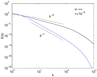
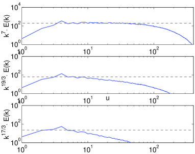
Figure 1: Energy spectra $E(k)=E^{u}(k)$ from a $4096^{2}$ simulation of the NS-$\alpha$ equations. (a): the blue line is the spectrum for NS-$\infty$, the black line for the NSE ($\alpha=0$). (b) top to bottom: the energy spectrum for NS-$\infty$ compensated by $k^{7},k^{19/3},\mbox{and }k^{17/3}$, respectively. The compensated spectrum in the top panel is flat in the range $6<k<40$, indicating the nominal range over which the $k^{-7}$ scaling holds.

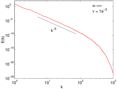
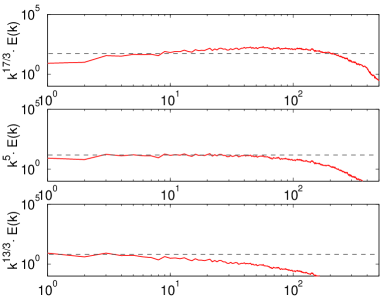
Figure 2: Energy spectrum $E(k)=E^{u}(k)$ from a $4096^{2}$ simulation of the Leray-$\alpha$ equations. (a): energy spectrum for the Leray-$\infty$. (b) top to bottom: energy spectrum of Leray-$\alpha$ compensated by $k^{17/3},k^{5},\mbox{and }k^{13/3}$, respectively. The compensated spectrum in the middle panel is flat in the range $7<k<50$, indicating the nominal range over which the $k^{-5}$ scaling holds.

3.2 Results for the Leray-$\infty$ equations

In Figures 2 and 2 we use the notation $E(k)$ for $E^{u}(k)$. In Figure 2 we present the main numerical results from [20] for the 2d NS-$\infty$ equations, showing the $k^{-7}$ scaling of the energy spectrum. In Figure 2 we show that the 2d Leray-$\infty$ energy spectrum attains a $k^{-5}$ power law in a $4096^{2}$ resolution simulation. From Table 1, the scaling $k^{-5}$ stems, based on the analytical arguments in section 2, from a characteristic time scale given by $\tau_{k}=\left(k\sqrt{{V}_{k}{U}_{k}}\right)^{-1}$, which is comparable to the inverse of the square root of the enstrophy of an eddy of the size $1/k$. To see this, recall from section 2 that the typical smoothed and unsmoothed velocity of eddy of size $\sim 1/k$ are given by

$${U}_{k} =\frac{1}{L^{2}}\left\langle\|u_{k,2k}(x)\|_{L^{2}(\Omega)}\right\rangle,$$ (21)

$${V}_{k} =\frac{1}{L^{2}}\left\langle\|v_{k,2k}(x)\|_{L^{2}(\Omega)}\right\rangle,$$ (22)

then, we can define

$$\mathcal{W}_{k} =\frac{1}{L^{2}}\left\langle\|\nabla\times u_{k,2k}\|_{L^{2}(\Omega)}\right\rangle,$$ (23)

$$Q_{k} =\frac{1}{L^{2}}\left\langle\|\nabla\times v_{k,2k}\|_{L^{2}(\Omega)}\right\rangle,$$ (24)

as the smoothed and unsmoothed enstrophy per unit area in the shell $[k,2k).$ Now, observe that

$$\tau_{k}=\left(k\sqrt{{V}_{k}{U}_{k}}\right)^{-1}\sim\left(\sqrt{{Q}_{k}{\mathcal{W}}_{k}}\right)^{-1}.$$

Therefore, the numerical results in Figure 2 clearly support our claim that the characteristic time scale $\tau_{k}=\left(k\sqrt{{V}_{k}{U}_{k}}\right)^{-1}$ determined by the dominant cascading quantity, namely the enstrophy $\int_{\Omega}q\cdot\omega\;dx$ for the 2d Leray-$\infty$ model, governs the dynamics of eddies in the subrange $k\alpha\gg 1$. This conclusion is consistent with our original prediction in [20] that, in general, the dominant cascading conserved quantity in the $\alpha$-model dictates the time scale associated with eddy of size $1/k$ and hence the power law of the energy spectrum $E^{u}(k)$ in the subrange $k\alpha\gg 1$.

4 Conclusion

The main goal of this study is to verify our claim in [20] about the choice of particular characteristic time scales of eddy of size $1/k$, for $k\alpha\gg 1$, for particular $\alpha$-model equations. Our results in [20] led us to conclude that the choice depends on the form of the cascading conserved enstrophy, which is the dominant forward cascading quantity. To verify this conclusion, we perform a high resolution simulation of the 2d Leray-$\alpha$ equations in the limit as $\alpha{\rightarrow}\infty$ similar to our study of the 2d NS-$\infty$ equations. We summarize the three steps to this study which verifies these claims:

1. Identify the conserved quantities (in the absence of viscosity and forcing) for 2d Leray-$\alpha$, and the dominant one in the forward cascade regime.

2. Calculate the power laws using semi-rigorous arguments as in [6, 8, 9, 11, 12, 16, 20]. This will give us the three possible power laws of the energy spectrum in the wavenumber regime $k\alpha\gg 1$.

3. Perform a high-resolution simulation to identify which one of the power laws of the energy spectrum calculated in step (ii) actually arise for the 2d Leray-$\alpha$ model.

   As we have speculated in [20], the scaling exponent in the wavenumber regime $k\alpha\gg 1$ will be governed by the time scale of the dominant cascading conserved quantity in that regime. If we extend the same argument to predict the scaling for the 3d NS-$\alpha$ and the 3d Leray-$\alpha$ model equations then we obtain the following predictions. Since $E^{uv}=\frac{1}{2}\int_{[0,L]^{3}}\tilde{u}\cdot\tilde{v}\;dx$ and $E^{vv}=\frac{1}{2}\int_{[0,L]^{3}}v\cdot v\;dx$ are the conserved energy which are the dominant cascading quantities for the 3d NS-$\alpha$ and 3d Leray-$\alpha$, respectively, then we predict the scaling of $E^{u}(k)\sim k^{-11/3}$ for the 3d NS-$\alpha$ (that is, steeper than the $k^{-3}$ proposed in [11]) and the scaling of $E^{u}(k)\sim k^{-17/3}$ for the 3d Leray-$\alpha$ (that is, steeper than the $k^{-13/3}$ suggested in [5] in the wavenumber regime $k\alpha\gg 1$. Our prediction of $k^{-17/3}$ power law corresponds to one of the power laws initially derived in [5] as candidate power law for the smoothed energy spectrum of the 3d Leray-$\alpha$ model. The verification of these possibilities in the 3d case will be explored in future work.

5 Acknowledgments

We are grateful to Mark A. Taylor for his continued collaboration on this study. E. Lunasin was supported by UC Irvine and the NSF grant no. DMS-0504619 when this work was initiated. S. Kurien was supported by the NNSA of the U.S. DOE at Los Alamos National Laboratory under contract no. DE-AC52-06NA25396, partially supported by the Laboratory Directed Research and Development program and the DOE Office of Science Advanced Scientific Computing Research (ASCR) Program in Applied Mathematics Research. The work of E. S. Titi was supported in part by the NSF grants no. DMS-0504619 and no. DMS-0708832, and the ISF grant no. 120/6.

6 References

References

- [1] S. Chen, C. Foias, D.D. Holm, E. Olson, E.S. Titi and S. Wynne, Camassa-Holm equations as a closure model for turbulent channel and pipe flow, Phys. Rev. Lett. 81 (1998), no. 24, 5338–5341.
- [2] S. Chen, C. Foias, D.D. Holm, E. Olson, E.S. Titi and S. Wynne, A connection between the Camassa-Holm equations and turbulent flows in channels and pipes, Phys. Fluids 11 (1999), no. 8, 2343–2353.
- [3] S. Chen, C. Foias, D.D. Holm, E. Olson, E.S. Titi and S. Wynne, The Camassa–Holm equations and turbulence, Phys. D 133 (1999), no. 1-4, 49–65.
- [4] S. Chen, D.D. Holm, L.G. Margolin and R. Zhang, Direct numerical simulations of the Navier–Stokes alpha model, Phys. D 133 (1999), no. 1-4, 66–83.
- [5] A. Cheskidov, D.D. Holm, E. Olson and E.S. Titi, On a Leray- model of turbulence, Royal Soc. A, Mathematical, Physical and Engineering Sciences, 461 (2005), 629–649.
- [6] C. Cao, D. Holm and E.S. Titi, On the Clark- model of turbulence: global regularity and long-time dynamics, Journal of Turbulence, 6 (2005), no. 20, 1–11.
- [7] R. Clark, J. Ferziger and W. Reynolds, Evaluation of subgrid scale models using an accurately simulated turbulent flow, J. Fluid Mech. 91, (1979), 1–16.
- [8] Y. Cao, E. Lunasin and E.S. Titi, Global well-posedness of the three-dimensional viscous and inviscid simplified Bardina turbulence models, Communications in Mathematical Sciences, 4, no. 4, (2006), 823–848.
- [9] C. Foias, What do the Navier–Stokes equations tell us about turbulence? Harmonic analysis and nonlinear differential equations (Riverside, CA, 1995), 151–180, Contemp. Math., 208, Amer. Math. Soc., Providence, RI, 1997.
- [10] C. Foias, D.D. Holm and E.S. Titi, The three-dimensional viscous Camassa–Holm equations, and their relation to the Navier-Stokes equations and turbulence theory, J. Dynam. Differential Equations 14 (2002), 1–35.
- [11] C. Foias, D.D. Holm and E.S. Titi, The Navier–Stokes–alpha model of fluid turbulence. Advances in nonlinear mathematics and science, Phys. D 152/153 (2001), 505–519.
- [12] C. Foias, O. Manley, R. Rosa and R. Temam, Navier–Stokes Equations and Turbulence, Cambridge University Press, Cambridge, 2001.
- [13] B. Geurts and D. Holm, Fluctuation effect on 3d-Lagrangian mean and Eulerian mean fluid motion, Physica D, 133 (1999), 215–269.
- [14] B. Geurts and D. Holm, Regularization modeling for large eddy simulation, Physics of Fluids, 15, (2003), L13-L16.
- [15] D. Holm, Marsden, and, T. Ratiu, Euler-Poincaré models of ideal fluids with nonlinear dispersion, Phys. Rev. Lett. 80, (1998), 4173–4176
- [16] A. Ilyin, E. Lunasin and E.S. Titi, A modified-Leray- subgrid scale model of turbulence, Nonlinearity, 19, (2006), 879–897.
- [17] A. Ilyin and E.S. Titi, Attractors for the two-dimensional Navier-Stokes- model: an -dependence study, Journal of Dynamics and Differential Equations, 14, No. 4, (2003), 751–778.
- [18] R.H. Kraichnan, Inertial ranges in two-dimensional turbulence, Phys. Fluids, 10, (1967), 1417-1423.
- [19] W. Layton and R. Lewandowski, On a well-posed turbulence model, Dicrete and Continuous Dyn. Sys. B, 6, (2006), 111-128.
- [20] E. Lunasin, S. Kurien, M.A. Taylor, and E.S. Titi, A study of the Navier-Stokes- model for two-dimensional turbulence, Journal of Turbulence, 8, (2007), 751–778.
- [21] K. Mohseni, B. Kosović, S. Shkoller and J. Marsden, Numerical simulations of the Lagrangian averaged Navier-Stokes equations for homogeneous isotropic turbulence, Phys. of Fluids, 15 (2003), No.2, 524–544.
- [22] B. Nadiga and S. Skoller, Enhancement of the inverse-cascade of energy in the two-dimensional averaged Euler equations, Phys. of Fluids, 13, (2001), 1528–1531.
- [23] E. Olson and E.S. Titi, Viscosity versus vorticity stretching: global well-posedness for a family of Navier-Stokes-alpha-like models, Nonlinear Anal., 66, (2007), No. 11, 2427–2458.