Magnetorotational instability in electrically driven fluids

Abstract

The linear stability of electrically driven flow of liquid metal in circular channel in the presence of vertical magnetic field is studied. It is shown that the instability threshold of such flow is determined by magnetorotational instability of non-axisymmetric modes ($m\neq 0$) and does not depend on the type of the fluid if magnetic Prandtl number is small $\textrm{Pr}\ll 1$. Our numerical results are found to be in a good agreement with available experimental data from Grenoble High Magnetic Field Laboratory, France [P. Moresco and T. Alboussière, J. Fluid Mech. 504, 167 (2004)].

The theoretical and experimental study of magnetorotational instability (MRI) has attracted much attention in recent years. MRI was originally predicted by Velikhov Velikhov (1959) in 1959, but its intensive study began only in 1991 when it was rediscovered in astrophysical context by Balbus and Hawley Balbus and Hawley (1991). At present time subject of MRI is one of the most important developments in magnetohydrodynamic (MHD) theory with far reaching consequences for a variety of astrophysical phenomena such as accretion disks Balbus and Hawley (1998); Balbus (2003), magnetic reconnection Coppi and Coppi (2001a) and dynamo Kersalé et al. (2004).

One of the topics of great current interest is experimental verification of MRI. Several experiments have been initiated to investigate MRI in laboratory Ji et al. (2001); Noguchi et al. (2002); Stefani et al. (2006); Sisan et al. (2004); Velikhov et al. (2006); Noguchi and Pariev (2003) by studying the stability of conducting fluid (liquid metal) rotating in transverse magnetic field. Despite these attempts, the MRI has never been clearly detected in laboratory and any progress in this direction is extremely important. Current status of experimental studies of MRI is described in Balbus (2006); Ji et al. (2006).

Two different mechanisms of the fluid rotation have been proposed for MRI experiments so far: mechanical drive by virtue of viscous drag force acting on the fluid between moving surfaces (Couette flow) and electrical drive by Ampere force arising when the electric current is passed through the fluid in transverse magnetic field (electrically driven flow). In most existing MRI experiments a Couette flow is used either in cylindrical Ji et al. (2001); Noguchi et al. (2002); Stefani et al. (2006) or spherical geometry Sisan et al. (2004). The main difficulty of the cylindrical Couette flow is the presence of the stationary end-caps that affect the entire equilibrium flow making it different from the idealized infinite-cylinder angular velocity profile $\Omega(r)=a+b/r^{2}$ so the conditions for MRI may not be met. Their influence can be reduced either by employing the differentially rotating end-caps Ji et al. (2006, 2004) or by using sufficiently long cylinders. In the latter case, experimental observations of MRI have been reported Stefani et al. (2006); Donnelly and Ozima (1960). MRI has also been observed in the experiment with rotating spheres Sisan et al. (2004) though the background flow was already fully turbulent without any magnetic field, indicating that MRI is not the only possible instability in this geometry.

Another way to rotate conducting fluid in circular channel with axial magnetic field is to apply radial electric current (Fig. 1). In this case the equilibrium flow forms so-called Hartmann layers near the top and bottom walls and parallel boundary layers near the side walls. The widths of these layers scale with Hartmann number Ha (see Eq. (1) for definition) as $O(\textrm{Ha}^{-1})$ and $O(\textrm{Ha}^{-1/2})$ respectively, so they become negligible at high values of magnetic field Baylis and Hunt (1971). Such flow has the angular velocity profile $\Omega(r)\propto 1/r^{2}$ almost entirely in the cross-section of the channel Khalzov and Smolyakov (2006). This profile is stable in hydrodynamics according to Raleigh’s criterion, but it can be destabilized in the presence of magnetic field since it satisfies the necessary condition for MRI $\partial\Omega^{2}(r)/\partial r<0$ Velikhov (1959). MRI experiment based on electrically driven flow of liquid sodium has been proposed in the Russian Research Center ”Kurchatov Institute” Velikhov et al. (2006) and built in Obninsk (Russia). A similar configuration using plasma instead of liquid metal has been developed in Los Alamos Noguchi and Pariev (2003). At present time experimental data are not available from those MRI experiments.

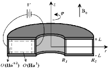
Figure 1: Sketch of electrically driven flow. Some details are shown as in Fig. 1 in Ref. Moresco and Alboussière (2004).

The electrically driven flow of liquid metal (mercury) in circular channel was also used in Grenoble High Magnetic Field Laboratory, France to investigate the stability of the Hartmann layers Moresco and Alboussière (2004). In this experiment a well-marked transition to turbulence was found when the ratio of Reynolds number to Hartmann number $\textrm{R}=\textrm{Re}/\textrm{Ha}$ exceeded critical value $\textrm{R}_{c}^{*}\approx 380$ (star denotes the quantities taken from Moresco and Alboussière (2004)), this value of $\textrm{R}_{c}^{*}$ was valid also for inverse process of laminarization without a visible hysteresis and for a wide range of intensities of the magnetic field ($\textrm{Ha}=100\div 1700$). The critical value $\textrm{R}_{c}^{*}$ obtained in Grenoble experiment is two orders of magnitude smaller than $\textrm{R}_{c}^{\textrm{Ha}}\approx 50,000$ predicted by the linear stability theory for Hartmann layers Lock (1955). A possible explanation to this paradox is discussed in papers Krasnov et al. (2004); Zienicke and Krasnov (2005), where a complicated two-step transition scenario to turbulence in the Hartmann layers is assumed. In these papers the radial dependence of the velocity profile in the main part of the flow is completely disregarded. In the present Letter, it is suggested however that in this configuration the magnetized flow can be destabilized via the MRI mechanism.

We study the linear stability of electrically driven flow of liquid metal in the geometries relevant to the Grenoble and Obninsk MRI experiments (Table 1) and show that the instability thresholds in these experiments are determined by MRI of global non-axisymmetric modes with large azimuthal mode numbers $m$. In our analysis we neglect all boundary layers and assume that the fluid rotates in the uniform axial magnetic field $\textbf{B}_{0}=B_{0}\textbf{e}_{z}$ with equilibrium velocity $\textbf{V}_{0}=r\Omega(r)\textbf{e}_{\varphi}$ where $\Omega(r)=M_{0}/r^{2}$ throughout the cross-section of the channel. The equilibrium angular momentum of the velocity $M_{0}$ is determined by the total electric current $I_{0}$ passing through the channel Khalzov and Smolyakov (2006):

$$M_{0}=\frac{I_{0}}{4\pi\sqrt{\rho\sigma\nu}},$$

where $\rho$, $\sigma$ and $\nu$ are fluid density, electric conductivity and kinematic viscosity respectively.

Table 1: Parameters of Grenoble and Obninsk experiments.

	$R_{1}$ (cm)	$R_{2}$ (cm)	$L$ (cm)	Fluid	Pr
Grenoble	4	5	0.5	Hg	$1.49\cdot 10^{-7}$
Obninsk	3	15	3	Na	$8.8\cdot 10^{-6}$

A number of similar studies was performed by different researches Ji et al. (2001); Noguchi et al. (2002); Shalybkov et al. (2002); Rüdiger et al. (2003), who considered the stability of more general idealized Couette flow $\Omega(r)=a+b/r^{2}$. The major part of these studies is restricted to the case of axisymmetric modes with $m=0$ Ji et al. (2001); Noguchi et al. (2002), which are known to have the largest growth rate of MRI. Numerical analysis of non-axisymmetric modes with small $m$ Shalybkov et al. (2002); Rüdiger et al. (2003) shows that they can have lower instability threshold (lower critical values of Reynolds number Re), so they might be easier to excite in real experiment. For electrically driven flow it was found recently Khalzov et al. (2006) that in ideal MHD the MRI threshold decreases with $m$ as $\textrm{Re}\propto 1/m$; therefore the most dangerous modes in such flow are those with larger $m$ (though they have smaller instability growth rate). Our present results suggest that overall stability of the flow in a finite height circular channel is determined by dissipative perturbations with large azimuthal numbers $m$.

We use dissipative incompressible MHD equations linearized about the equilibrium state and represent all perturbations in the form $f(r,z)\exp(\gamma t+im\varphi)$ in cylindrical system of coordinates $\{r,\varphi,z\}$. It should be stressed here that we consider the channel of the finite height – this is a substantial difference of our stability analysis from previous studies. For computational convenience we introduce dimensionless quantities, taking as a unit of length a half-height of the channel $L$ and as a unit of time the characteristic viscous time $L^{2}/\nu$. The perturbations of velocity $\delta\textbf{V}$ and magnetic field $\delta\textbf{B}$ can be written in terms of dimensionless vectors v and h as

$$\delta\textbf{V}=\frac{M_{0}}{L}\textbf{v},~{}~{}~{}\delta\textbf{B}=B_{0}\frac{\textrm{Pr}\textrm{Re}}{\textrm{Ha}}\textbf{h},$$

where

$$\textrm{Ha}=\frac{LB_{0}}{c}\sqrt{\frac{\sigma}{\rho\nu}},~{}~{}~{}\textrm{Re}=\frac{M_{0}}{\nu},~{}~{}~{}\textrm{Pr}=\frac{4\pi\sigma\nu}{c^{2}}$$ (1)

are Hartmann, Reynolds and magnetic Prandtl numbers respectively. Introducing vortex $\mbox{\boldmath$\bf\omega$}=\nabla\times\textbf{v}$ we arrive at

$$\gamma{\mbox{\boldmath$\bf\omega$}} = \nabla^{2}\mbox{\boldmath$\bf\omega$}-\frac{im\textrm{Re}}{r^{2}}\mbox{\boldmath$\bf\omega$}-\frac{2\textrm{Re}}{r^{2}}\omega_{r}\textbf{e}_{\varphi}+\textrm{Ha}\nabla\times\textbf{h}^{\prime}_{z},$$ (2)

$$\textrm{Pr}\gamma\textbf{h} = \nabla^{2}\textbf{h}-\frac{im\textrm{Pr}\textrm{Re}}{r^{2}}\textbf{h}-\frac{2\textrm{Pr}\textrm{Re}}{r^{2}}h_{r}\textbf{e}_{\varphi}+\textrm{Ha}\textbf{v}^{\prime}_{z},$$ (3)

where prime denotes the derivative with respect to $z$. Note that $r$ and $\varphi$ components of these equations are enough to find the full solution ($z$-components can be deduced from the conditions $\nabla\cdot\mbox{\boldmath$\bf\omega$}=0$ and $\nabla\cdot\textbf{h}=0$).

The proper boundary conditions should be specified prior to solving the system (2), (3). In the flow of viscous fluid all velocity components vanish at the rigid walls, i. e.

$$\textbf{v}|_{r=r_{1},r_{2}}=0,~{}~{}~{}\textbf{v}|_{z=\pm 1}=0,$$ (4)

The boundary conditions for magnetic field depend on the conductivity of the walls. In both Grenoble and Obninsk experiments the side walls of the channel can be considered as perfect conducting. At the surface of the perfect conductor the time-varying normal component of magnetic field as well as the tangential components of electric current should be zero. This means

$$h_{r}|_{r=r_{1},r_{2}}=0,~{}~{}~{}\frac{\partial(rh_{\varphi})}{\partial r}\bigg{|}_{r=r_{1},r_{2}}=0.$$ (5)

The other two walls (Hartmann walls) are electrical insulators. For simplicity we assume that the perturbed components of the field are zero at these walls, i. e.

$$h_{r}|_{z=\pm 1}=0,~{}~{}~{}h_{\varphi}|_{z=\pm 1}=0,$$ (6)

which is consistent with the absence of the normal component of the current at the surface of insulator.

Equations (2), (3) with boundary conditions (4)-(6) constitute an eigenvalue problem with $\gamma$ being an unknown eigenvalue. A solution to this problem was sought by expanding functions $v_{r}$, $v_{\varphi}$, $h_{r}$ and $h_{\varphi}$ in terms of either odd or even polynomials in $z$ (up to $N_{z}=8$), and by discretization of the system (2), (3) in terms of finite differences in $r$-direction (up to $N_{r}=50$). Then this system was reduced to a large ($4N_{r}N_{z}\times 4N_{r}N_{z}$) matrix eigenvalue problem which was solved using standard numerical methods of MATLAB.

The following numerical procedure was performed for two values of magnetic Prandtl number corresponding to mercury (Hg) and liquid sodium (Na) and for the geometries of both Grenoble and Obninsk experiments (Table 1). Taking a value of azimuthal number from the array $m=0\div 200$, we scanned through a range of values of Re and Ha, finding the maximal growth rate for given parameters. For each value of Ha we determined the value of Re that yields a marginal stability, i. e. corresponds to the zero maximal growth rate $\textrm{Re}(\gamma)=0$. Thus we obtained the marginal stability curves at the plane $\textrm{Re}-\textrm{Ha}$ (Fig. 2, 3).

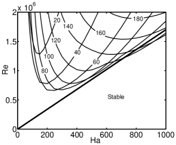
Figure 2: Calculated marginal stability curves for geometry of Grenoble experiment. Azimuthal mode numbers $m$ are shown. Difference between Hg and Na is within the line width. Straight line corresponds to the transition to turbulence observed in experiment $\textrm{Re}=1,700\textrm{Ha}$.

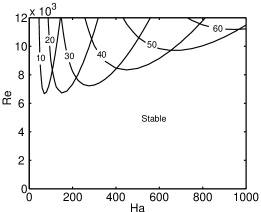
Figure 3: Calculated marginal stability curves for geometry of Obninsk experiment. Azimuthal mode numbers $m$ are shown. Difference between Hg and Na is within the line width.

One can see from Fig. 2 and 3 that the instability threshold is determined by different azimuthal modes at different Hartmann numbers Ha. For larger Ha the corresponding $m$ is larger. In fact, a simple scaling law can be obtained for large $m$: $\textrm{Ha}\propto m^{2}$. The stability curves of axisymmetric modes with $m=0$ are not shown because they are situated at much higher values of Re. Therefore, the non-axisymmetric modes play the decisive role for excitation of MRI in electrically driven flow.

It is worth noting here that the marginal stability curves practically do not depend on the magnetic Prandtl number Pr of the fluid; they are determined only by the geometry of the channel. This is true for non-axisymmetric modes in the limit $\textrm{Pr}\ll 1$ which is common for most liquid metals. In this case a good approximation for instability threshold can be achieved by neglecting all the terms containing Pr in the Eq. (3) and reducing the system (2), (3) to one vector equation with hydrodynamical variables. Such approach is not applicable for axisymmetric modes in axial magnetic field Herron and Goodman (2006).

In ideal MHD, the MRI threshold to a significant degree is affected by singularities inherent in eigen-value problem Coppi and Coppi (2001b). In incompressible limit, the MRI of non-axisymmetric modes is associated with one set of these singularities – the so-called Alfven resonances Khalzov et al. (2006). Within the frame of MHD model considered here, the Alfven resonances are removed by dissipative effects (resistivity and viscosity). An important consequence of this is that the dissipative stability threshold for non-axisymmetric modes appears to be lower than the ideal one, i. e. the dissipation (mainly the resistivity) has destabilizing effect on the ideal modes.

Our main observation is that the MRI threshold of the electrically driven flow is formed by the envelope of all marginal stability curves corresponding to modes with different azimuthal numbers $m$. The shape of the envelope depends on the particular geometry of the channel (see Fig. 2 and 3). In the Fig. 2, the envelope is close to the form $\textrm{Re}\propto\textrm{Ha}$ when $\textrm{Ha}\gtrsim 300$. It means that instability should be excited in this geometry if the ratio $\textrm{R}=\textrm{Re}/\textrm{Ha}$ exceeds some critical value $\textrm{R}_{c}$. As mentioned above this effect was actually detected experimentally Moresco and Alboussière (2004).

For comparison of our numerical results with the experimental data we need to calculate $\textrm{R}_{c}$ taking into account our definition of Reynolds number (1). The relation between Reynolds number $\textrm{Re}^{*}$ from Ref. Moresco and Alboussière (2004) and Re used in our calculations is

$$\textrm{Re}^{*}=\frac{dv_{m}}{\nu}=\frac{2LM_{0}}{\nu(R_{2}-R_{1})}\ln\frac{R_{2}}{R_{1}}\approx 0.22\textrm{Re},$$

where $d=2L$ is the channel height and $v_{m}$ is the mean velocity in the equilibrium flow. Our definition of Ha is the same as definition of Ha from Ref. Moresco and Alboussière (2004) used in the figures (though it is not the same as stated in Eq. (2.4) in Ref. Moresco and Alboussière (2004)). Thus we obtain

$$\textrm{R}_{c}=\frac{\textrm{Re}}{\textrm{Ha}}\approx\frac{1}{0.22}\textrm{R}_{c}^{*}\approx 1700.$$

The line associated with this experimental value of $\textrm{R}_{c}$ is also plotted in Fig. 2. As one can see, the calculated threshold of MRI is in a good agreement with the experimental results.

A natural question arises: what do we observe in reality – MRI or Hartmann layer instability? A strong argument for MRI is the comparison of respective linear instability thresholds: MRI threshold found in our calculations corresponds to that measured in the Grenoble experiment and two orders of magnitude smaller than instability threshold of Hartmann layers Lock (1955). Also it is evident that in the presence of global (affecting the entire flow) robust linear instability such as MRI the nonlinear effects in Hartmann layers Krasnov et al. (2004); Zienicke and Krasnov (2005) are unlikely to play the major role in destabilizing the flow. The global character of MRI is illustrated in Fig. 4 where a typical marginally stable eigenfunction $v_{\varphi}$ is shown.

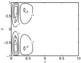
Figure 4: Calculated contours of marginally stable eigenfunction $v_{\varphi}$ in cross-section of Grenoble channel at $m=100$, $\textrm{Ha}=500$, $\textrm{Re}=9\cdot 10^{5}$. Magnitude is shown in arbitrary units.

In conclusion, we have shown that the instability threshold in electrically driven flow is determined by MRI of global non-axisymmetric modes with large azimuthal mode numbers $m$. This threshold does not depend on the type of conducting fluid as long as the magnetic Prandtl number of the fluid is small $\textrm{Pr}\ll 1$. MRI threshold calculated for the geometry of the Grenoble experiment agrees well with the critical ratio $\textrm{R}_{c}$ found in this experiment. These results suggest that the transition to turbulence observed in the experiment Moresco and Alboussière (2004) is associated with non-axisymmetric MRI in electrically driven flow.

This work is supported in part by NSERC Canada.

References

- Velikhov (1959) E. P. Velikhov, Sov. Phys. JETP 36, 995 (1959).
- Balbus and Hawley (1991) S. A. Balbus and J. F. Hawley, Astrophys. J. 376, 214 (1991).
- Balbus and Hawley (1998) S. A. Balbus and J. F. Hawley, Rev. Mod. Phys. 70, 1 (1998).
- Balbus (2003) S. A. Balbus, Annu. Rev. Astron. Astrophys. 41, 555 (2003).
- Coppi and Coppi (2001a) B. Coppi and P. S. Coppi, Phys. Rev. Lett. 87, 051101 (2001a).
- Kersalé et al. (2004) E. Kersalé, D. W. Hughes, G. I. Ogilvie, S. M. Tobias, and N. O. Weiss, Astrophys. J. 602, 892 (2004).
- Ji et al. (2001) H. Ji, J. Goodman, and A. Kageyama, Mon. Not. R. Astron. Soc. 325, L1 (2001).
- Noguchi et al. (2002) K. Noguchi, V. I. Pariev, S. A. Colgate, H. F. Beckley, and J. Nordhaus, Astrophys. J. 575, 1151 (2002).
- Stefani et al. (2006) F. Stefani, T. Gundrum, G. Gerbeth, G. Rüdiger, M. Schultz, J. Szklarski, and R. Hollerbach, Phys. Rev. Lett. 97, 184502 (2006).
- Sisan et al. (2004) D. R. Sisan, N. Mujica, W. A. Tillotson, Y.-M. Huang, W. Dorland, A. B. Hassam, T. M. Antonsen, and D. P. Lathrop, Phys. Rev. Lett. 93, 114502 (2004).
- Velikhov et al. (2006) E. P. Velikhov, A. A. Ivanov, S. V. Zakharov, V. S. Zakharov, A. O. Livadny, and K. S. Serebrennikov, Phys. Lett. A 358, 216 (2006).
- Noguchi and Pariev (2003) K. Noguchi and V. I. Pariev, AIP Conf. Proc. 692, 285 (2003), eprint astro-ph/0309340.
- Balbus (2006) S. A. Balbus, Nature 444, 281 (2006).
- Ji et al. (2006) H. Ji, M. Burin, E. Schartman, and J. Goodman, Nature 444, 343 (2006).
- Ji et al. (2004) H. Ji, J. Goodman, A. Kageyama, M. Burin, E. Schartman, and W. Liu, AIP Conf. Proc. 733, 21 (2004).
- Donnelly and Ozima (1960) R. J. Donnelly and M. Ozima, Phys. Rev. Lett. 4, 497 (1960).
- Baylis and Hunt (1971) J. A. Baylis and J. C. R. Hunt, J. Fluid Mech. 48, 423 (1971).
- Khalzov and Smolyakov (2006) I. V. Khalzov and A. I. Smolyakov, Technical Physics 51, 26 (2006).
- Moresco and Alboussière (2004) P. Moresco and T. Alboussière, J. Fluid Mech. 504, 167 (2004).
- Lock (1955) R. C. Lock, Proc. R. Soc. Lond. A 233, 105 (1955).
- Krasnov et al. (2004) D. S. Krasnov, E. A. Zienicke, O. Zikanov, T. Boeck, and A. Thess, J. Fluid Mech. 504, 183 (2004).
- Zienicke and Krasnov (2005) E. A. Zienicke and D. S. Krasnov, Phys. Fluids 17, 114101 (2005).
- Shalybkov et al. (2002) D. Shalybkov, G. Rüdiger, and M. Schultz, Astron. Astrophys. 395, 339 (2002).
- Rüdiger et al. (2003) G. Rüdiger, M. Schultz, and D. Shalybkov, Phys. Rev. E 67, 046312 (2003).
- Khalzov et al. (2006) I. V. Khalzov, V. I. Ilgisonis, A. I. Smolyakov, and E. P. Velikhov, Phys. Fluids 18, 124107 (2006).
- Herron and Goodman (2006) I. Herron and J. Goodman, Z. Angew. Math. Phys. 57, 615 (2006).
- Coppi and Coppi (2001b) B. Coppi and P. S. Coppi, Ann. Phys. 291, 134 (2001b).