Perturbative Treatment of Symmetry Breaking Within Random Matrix Theory

Abstract

We discuss the applicability, within the Random Matrix Theory, of perturbative treatment of symmetry breaking to the experimental data on the flip symmetry breaking in quartz crystal. We found that the values of the parameter that measures this breaking are different for the spacing distribution as compared to those for the spectral rigidity. We consider both twofold and threefold symmetries. The latter was found to account better for the spectral rigidity than the former. Both cases, however, underestimate the experimental spectral rigidity at large L. This discrepancy can be resolved if an appropriate number of eigenfrequecies is considered to be missing in the sample. Our findings are relevant to isospin violation study in nuclei.

The study of wave chaos using acoustic resonators Weaver ,Tanner supplies an invaluable additional test of Random Matrix Theory (RMT) Meht ; Meht1 . In a 1996 paper Ellegaard et al.Elleg , studied the gradual breaking of the presumed twofold flip symmetry of a quartz crystal by removing an octant of a sphere of an increasing radius at one of the corners and analysing the statistics of the resulting acoustic eigenfrequencies. They found a gradual evolution of the spacing distribution from that of two uncoupled Gaussian Othogonal Ensembles (2GOE) when the crystal is an uncut perfect rectangle, into a single GOE, when a large chunk of the crystal is removed from one of the corners of the rectangle. This constituted a complete breaking of the symmetry present in the crystal in the uncut situation. The spectral rigidity, measured by Dyson’s $\Delta_{3}(L)$ was also measured in this reference. The 2 uncoupled GOE’s was found to underestime by a great amount the large-$L$ data. This was attributed to pseudointegrable trajectories that do not suffer from the symmetry breaking. This point was further analysed by Abul . Using techniques developed by Pandey Pandey:1995 , Leitner Leitner treated the symmetry breaking problem with RMT-perturbation. He addressed only the spacing distribution. This work was further extended to the spectral rigidity in Abul-Magd:2004 . In all of the above treatment of the data of Elleg , the assumption was made that the uncut crystal has a twofold flip symmetry and thus is describable by two uncoupled GOE’s. The treatment of Leitner Leitner is found to describe fairly well the NNL distribution, but fails for the spectral rigidity, in contrast to the exact numerical simulation using the Deformed Gaussian Orthogonal Ensemble DGOE , recently performed in last . In this paper we further analyse the perturbative treatment of symmetry breaking within RMT. We find that the data of Elleg can be accounted for with 3GOE’s which are gradually mixed till a 1GOE limit is attained. We further find that that if some levels were missing in the sample of eigenfrequecies whose statistics is analysed, the $\Delta_{3}(L)$ can be very well accounted for even at large L without the need for pseudointegrable trajectories, whose calculation is difficult.

Using appropriate perturbative methods Leitner Leitner was able to find a formula for the nearest neighbor distributio (NND) which contains the symmetry braking term. He started basically with the formula for the nearest neigbhour spacing distribution for the superposition of $m$ GOE’s block matrices Meht

$$P_{m}(s)=\frac{d^{2}}{ds^{2}}E_{m}(s)$$ (1)

where, for the case of all block marices having the same dimension one has

$$E_{m}(s)=\left(E_{1}(\frac{s}{m})\right)^{m},$$ (2)

$$E_{1}(x)=\int_{x}^{\infty}(1-F(t))\,dt,$$ (3)

$$F(t)=\int_{0}^{t}P_{1}(z)\,dz.$$ (4)

In the above $P_{1}(z)$ is the normalized nearest neighbour spacing distribution of one block matrix. It is easy to find for $P_{m}(s)$, the following

$$P_{m}(s) = \frac{1}{m}\left[\left(E_{1}(s/m)\right)^{m-1}P_{1}(s/m)+(m-1)(E_{1}(s/m))^{m-2}(1-F(s/m))^{2}\right]$$ (5)

$$\equiv P^{(1)}_{m}(s)+P_{m}^{(2)}(s)$$ (6)

If all the block matrices belong to the GOE, then one can use the Wigner form for $P_{1}(z)$

$$P_{1}(z)=\frac{\pi}{2}ze^{-\frac{\pi}{4}z^{2}}\approx\frac{\pi}{2}z,$$ (7)

thus

$$F_{1}(z)=1-e^{-\frac{\pi}{4}z^{2}}\approx\frac{\pi}{4}z^{2},$$ (8)

$$E_{1}(z)=erfc\left(\frac{\sqrt{\pi}}{2}z\right)\approx 1-z.$$ (9)

where the large-$z$ limits of Eqs. (7)-(9) are also indicated above. It is now clear that the above expression for $P_{m}(s)$, (5) and (6), contains a term $P_{m}^{(1)}(s)$ with level repulsion, indicating short-range correlation among levels pertaining to the same block matrix and a second term $P_{m}^{(2)}(s)$ with no level repulsion, implying short-range correlation among NND levels pertaining to different blocks. Notice that for very small spacing, $P_{m}(s)$ behaves as

$$P_{m}(s)\approx\frac{\pi}{2m^{2}}s+\frac{m-1}{m}$$ (10)

for $m=1$, we get the usual $P_{1}(0)=0$, while for $m>1$, we get $P_{m}(0)=(m-1)/m$.

To account for symmetry breaking, Leitner Leitner considered the mixing between levels pertaining to nearest neigbhour block matrices and entails using the $2x2$ $P(s)$ distribution with full mixing. The DGOE result for the 2X2 matrix was derived in Carneiro:1991 and the resulting $P(s)$ is a product of a Poissonian term times a mixing term. Leitner’s procedure Leitner amounts to multiply the factor $P_{m}^{(2)}(s)$ of Eq. (6) by only the mixing term of the 2x2 $P(s)$ of Carneiro:1991 with the mixing parameter $\Lambda$ given by Pandey:1995 , $\Lambda=\lambda^{2}{\rho^{2}}$, with $\lambda^{2}$ being the ratios of the variances of the matrix elements within a block matrix to that of matrix elements pertaining to neighbouring off diagonal block matrices., and $\rho$ is the density of eigenfrequencies. Thus, he found, assuming that $\Lambda<<1$,

$$P_{m}(s,\Lambda)=P_{m}^{(1)}(s)+P_{2\times 2}(s,\Lambda)P_{m}^{(2)}(s).$$ (11)

where $P_{2\times 2}(s,\Lambda)$ is given by Leitner

$$P_{2\times 2}(s,\Lambda)=\sqrt{\frac{\pi}{8\Lambda}}I_{0}(\frac{s^{2}}{16\Lambda})\exp\left(-\frac{s^{2}}{16\Lambda}\right),$$ (12)

where $I_{0}$ is the modified Bessel function of order $0$. Though $P_{m}(s)$ is normalized, $P_{m}(s,\Lambda)$ is not. Accordingly one supplies coefficients $c_{N}$ and $c_{D}$, such that

$$P_{m}(s,\Lambda,c_{N},c_{D})\equiv c_{N}P_{m}(c_{D}s,\Lambda)$$ (13)

is normalized to unity. Similarly, $<s>$ should be unity too. Eq. (11) can certainly be generalized to consider the effect of mixing of levels pertaining to next to nearest neighbour blocks, and accordingly, $P_{3\times 3}(s,\Lambda)$, given in Ref. Carneiro:1991 would be used in Eq. (11) instead of $P_{2\times 2}(s,\Lambda)$. In the following, however, we use Eqs. (11), (13) as Leitner did Leitner .

In Ref. Leitner , Leitner also obtained approximate expression for the spectral rigidity $\Delta_{3}(L)$ using results derived by French et al. French . Leitner’s approximation to $\Delta_{3}$ is equal to the GOE spectral rigidity plus perturbative terms, that is

$$\Delta_{3}^{(m)}(L;\Lambda) \approx \Delta_{3}(L;\infty)+\frac{m-1}{\pi^{2}}\left[\left(\frac{1}{2}-\frac{2}{\epsilon^{2}L^{2}}-\frac{1}{2\epsilon^{4}L^{4}}\right)\right.$$ (14)

$$\times\ln(1+\epsilon^{2}L^{2})+\frac{4}{\epsilon L}\tan^{-1}(\epsilon L)+\left.\frac{1}{2\epsilon^{2}L^{2}}-\frac{9}{4}\right],$$

where

$$\epsilon = \frac{\pi}{2(\tau+\pi^{2}\Lambda)}$$ (15)

For the cut off parameter we use the value Abul-Magd:2004 $\tau=c_{m}e^{\pi/8-\gamma-1},$ where $c_{m}=m^{m/(m-1)}$ and $\gamma\approx 0.5772$ is Euler’s constant. This choice guarantees that when the symmetry is not broken, $\Lambda=0$, $\Delta_{3}^{(m)}(L,0)=m\Delta_{3}(L/m,\infty)$. In Ref. Leitner:1997 , Leitner fitted Eq. (13) for $m$=2 to the NND from Ref. Elleg , however, he did not fit the spectral rigidity. It is often the case that there are some missing levels in the statistical sample analysed. Such a situation was addressed recently by Bohigas and Pato ML . These authors have started from the general expression of $\Delta_{3}(L)$ derived by Dyson and Mehta Meht1 , namely,

$$\Delta_{3}(L)=\frac{L}{15}-\frac{1}{15L^{4}}\int_{0}^{L}~{}dx\big{(}L-x)^{3}(2L^{2}-9xL-3x^{4}\big{)}Y_{2}(x),$$ (16)

where the two-point cluster function, $Y_{2}(x_{1},x_{2})$, which owing to translational invariance becomes a function of the difference $x=\mid x_{1}-x_{2}\mid$, is defined by the usual expression,

$$Y_{2}(x_{1},x_{2})=1-\frac{R_{2}(x_{1},x_{2})}{R_{1}(x_{1})R_{1}(x_{2})},$$ (17)

where $R_{2}$ is the 2-point correlation function and $R_{1}$ is the density of the spectrum.

If a fraction, $1-g$, of the levels were actually analysed , the cluster function remains invariant, apart from a rescaling of the relevant variables, when the unfolded spactrum is employed, namely

$$Y_{2}^{g}(x_{1},x_{2})=1-\frac{(1-g)^{2}R_{2}(x_{1}^{g},x_{2}^{g})}{(1-g)R_{1}(x_{1}^{g})(1-g)R_{1}(x_{2}^{g})}=Y_{2}(x_{1}^{g},x_{2}^{g}),$$ (18)

where the scaled variables $x_{i}^{g}$ are just $\frac{x_{i}}{(1-g)}$

Using the above equation for the cluster function in the general expression for $\Delta_{3}(L)$, we obtain the Missing-Level (ML) expression of ML

$$\Delta_{3}^{g}(L)=g\frac{L}{15}+(1-g)^{2}\Delta_{3}\left(\frac{L}{1-g}\right).$$ (19)

In the application to our current problem of $m$-coupled GOE’s, the above formula continue to be valid since the basic input into its derivation, namely the invariance of $Y_{2}$, apart from the scaling of the argument $x$ into $x^{g}$, is quite general. Accordingly, we have the desired ML formula of $\Delta_{3}(L)$ for $m$-coupled GOE’s,

$$\Delta_{3}^{(m)g}(L;\Lambda)=g\frac{L}{15}+(1-g)^{2}\Delta_{3}^{(m)}\left(\frac{L}{1-g};\Lambda\right).$$ (20)

The presence of the linear term, even if small, could explain the large $L$ behavior of the measured $\Delta_{3}(L)$. We call this effect the Missing Level (ML) effect. Another possible deviation of $\Delta_{3}$ from Eq. (14) could arise from the presence of pseudo-integrable effect (PI) Abul ; bis2 . This also modifies $\Delta_{3}$ by adding a Poisson term just like Eq. (20).

The results of our analysis are shown in figures 1 and 2. In Fig. 1, the sequence of six measured NNDs were fitted for $m=2$ and $m=3.$ It can be seen that the Leitner model with three coupled GOE’s give a comparable and in some cases even better fit than the $m=2$ one. Figure 1a in fact shows a rather sharp peak in our calculated $P(s)$ for $m=3$, $P_{3}(s,0.0056)$. We consider this a failure of the Leitner formula (13) for the uncut crystal. In fact, a more appropriate description of the uncut crystal is to take $\Lambda=0$, namely a superposition of 3 uncoupled GOE’s, which works almost as good as the 2 uncoupled GOE’s description. The other parts of figure 1, $(b)-(x)$ seem to show the same insensitivity of $P_{m}(s,\Lambda)$ to $m$; the number of matrix blocks used in DGOE description. It is this insensitivity of the short-range nearest neighbour level correlation, measured by the spacing distribution, to the assumed symmetry inherent in the uncut crystal (and thus the number uncoupled GOE’s employed to describe it) that forces us to examine the long-range level correlation, namely spectral rigidity, “measured” by Dyson’s $\Delta_{3}$ statistics.

In Fig. 2. the $\Delta$-statistic was fitted with equation (14). It is clear from the figure that a good fit to the data of Ref. Elleg is obtained with $m=3$ for the values of $\Lambda$ given in table 1. This is to be contrasted with the case of $m=2$ which, according to Eq. (14) results in $\Delta_{3}^{(2)}(L,\Lambda)$ that is always below the one with $\Lambda=0$, $\Delta_{3}^{(2)}(L,0)$, which itself is always below the data points of Ref. Elleg . For this reason, only the $\Delta_{3}^{(2)}(L,0)$ is shown in the figure. It should be noted that the $\Delta$-statistics of the uncut crystal, Fig. 2a is very well described by that of 3 uncoupled GOE’s, namely $\Delta_{3}^{(3)}(L)=3\Delta_{3}^{(1)}(L/3)$ which is always larger than the above mentioned $\Delta_{3}^{(2)}(L)=2\Delta_{3}^{(1)}(L/2)$. The most conspicuous exception is Fig. 2b which corresponds to $r=0.5\,mm$ and where $1414$ frequency eigenvalues were found. We consider this a potential ML case and take for $\Delta_{3}$, the expression given in Eq. (20) and use it in Eq. (14) with $g$ taken as a parameter. The results are shown in Fig. 3. We find perfect fit to the data, if $g$ is taken to be $6\%$, namely only $94\%$ of the eigenfrequencies were in fact taken into account in the statistical analysis. In contrast, if 2GOE is used we still do not get very good agreement even if 18% of the levels are taken to be missing. There is, threfore, room to account much better for all cases (Fig. $2a$, $2c$, $\ldots$ ) in the 3GOE description, by appropiately choosing the correponding value of $g$. This is not the case if a 2GOE description is employed.

Table 1: Values of $\Lambda$ obtained by fitting Eqs. (13) and (14) respectively to the experimental NNDs and spectral rigidities from Ref. Elleg .

	$P(s)$			$\Delta_{3}(L)$
Data Set	Ref. Leitner:1997	Eq. (13) $m$=2	Eq. (13) $m$=3	Eq. (14) $m$=3
(a)	0.0013	0.0030	0.0067	0.0056
(b)	0.0054	0.0063	0.0098	0.0016
(c)	0.0096	0.010	0.017	0.0017
(d)	0.0313	0.032	0.064	0.027
(e)	0.0720	0.070	0.13	0.050
(f)	0.113	0.12	0.30	0.16
(x)	0.138	0.13	0.34	2.4

In conclusion, the perturbative tratment of symmetry breaking within RMT is assessed by using it to describe the coupling of $m$-fold symmetry The particular threefold case is used to analyse data on eigenfrequencies of elastomechanical vibration of a anisotropic quartz block. The treatment of Leitner Leitner is found to describe fairly well the NNL distribution, but fails for the spectral rigidity, in contrast to the exact numerical simulation using the Deformed Gaussian Orthogonal Ensemble recently performed in last . However, by properly taking into account the ML effect we have shown that the $\Delta_{3}(L)$, become closer to the data.

We have also verified that if a 2GOE description is used, namely, $m=2$ , then an account of the large-$L$ behaviour of $\Delta_{3}$ can also be obtained if a much larger number of levels were missing in the sample. In our particular case of Fig. 2b, we obtained $g=0.18$. This is 3 times larger than the ML needed in the 3GOE description. One major issue in the perturbative approach is the need to use different sets of values of the mixing parameter $\Lambda$ for the NNL distribution, $P(s)$, and for the $\Delta_{3}(L)$. Further study of this approach is certainly required. Finally, we mention that the perturbation approach to symmetry violation study within RMT of the type discussed in this paper may be valuable to isospin breaking in nuclei. In Ref. Mitch0 the breaking of isospin was studied in the case of the nucleus ²⁶Al where both T = 0 and 1 states are present in the low lying spectrum, which required the use of 2GOE description. Other, heavier, odd-odd nuclei may exhibit a spectrum where T = 2 states may also be present, requiring a 3GOE description of the isospin symmetry breaking. Work along these lines is in progress.

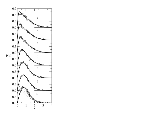
Figure 1: Nearest Neighbour Distributions. Histograms show data (a)-(x) from Ref. Elleg . Thin and thick solid lines show fits to the data carried out using Eq. (13) with m=2 and m=3 respectively. In graph (x) the long-dashed line is the Poisson distribution, the dot-dashed line is the Wigner distribution and the dashed and dotted lines are the respective distributions for superpositions of 2 and 3 uncoupled GOEs. See Table I for the values of $\Lambda$ obtained from the fits and the text for details.

Figure 2: Spectral Rigidities. Circles show data (a)-(x) from Ref. Elleg . Thick solid lines show fits to the data carried out using Eq. (13) with m=3. The dot-dashed line is the GOE spectral rigidity and the dashed and dotted lines are the respective rigidities for superpositions of 2 and 3 uncoupled GOEs. See Table I for the values of $\Lambda$ obtained from the fits.

Figure 3: Missing Levels. Full line corresponds to $\Delta_{3}(L)$ for the 3 GOE’s of Fig 2b with g = 0.06, while the dashed line corresponds to to the 2 GOE’s with g = 0.18. The data points corresponding to the case with r = 0.5 mm, are from fig 2b of Elleg

References

- (1) R. L. Weaver, J. Acoustic. Soc. Am. 85, 1005 (1989).
- (2) For a recent review of wave chaos in acoustics, see: G. Tanner and N. Sondergaard, J. Phys. A: Math. Theor., 40 R443 (2007)
- (3) M.L. Mehta, Random Matrices 2nd Edition (Academic Press, Boston, 1991); T.A. Brody et al., Rev. Mod. Phys. 53, 385 (1981); O. Bohigas, M. J. Giannoni and C. Schmit, Phys. Rev. Lett. 52, 1 (1984); O. Bohigas and M. J. Giannoni, in Mathematical and Computational Methods in Nuclear Physics, edited by J. S. DeHesa, J. M. Gomez and A. Polls, Lecture Notes in Physics Vol. 209 (Springer-Verlag, New York, 1984); T. Guhr, A. Müller-Groeling and A. Weidenmüller, Phys. Rep. 299, 189 (1998).
- (4) F. J. Dyson and M. L. Mehta, J. Math. Phys. 4, 701 (1963).
- (5) M. S. Hussein, and M. P. Pato, Phys. Rev. Lett. 70, 1089 (1993); M. S. Hussein, and M. P. Pato, Phys. Rev. C 47, 2401 (1993); M. S. Hussein, and M. P. Pato, Phys. Rev. Lett. 80, 1003 (1998).
- (6) C. E. Carneiro, M. S. Hussein and M. P. Pato, in H. A. Cerdeira, R. Ramaswamy, M. C. Gutzwiller and G. Casati (eds.) Quantum Chaos, p. 190 (World Scientific, Singapore) (1991).
- (7) C. Ellegaard, T. Guhr, K. Lindemann, H. Q. Lorensen, J. Nygard and M. Oxborrow, Phys. Rev. Lett. 75, 1546 (1995).
- (8) C. Ellegaard, T. Guhr, K. Lindemann, J. Nygard and M. Oxborrow, Phys. Rev. Lett. 77, 4918 (1996).
- (9) P. Bertelsen, C. Ellegaard, T. Guhr, M. Oxborrow and K. Schaadt, Phys. Rev.Lett. 83, 2171 (1999).
- (10) A. Abd El-Hady, A. Y. Abul-Magd, and M. H. Simbel, J. Phys. A 35, 2361 (2002).
- (11) A. Pandey, Chaos, Solitons and Fractals 5 (1995) 1275.
- (12) D. M. Leitner, Phys. Rev. E 48, 2536 (1993).
- (13) A.Y. Abul-Magd and M.H. Simbel, Phys. Rev. E 70 (2004) 046218.
- (14) J. B. French, V. K. B. Kota, A. Pandey and S. Tomsovic, Ann. Phys. (NY) 181, 198 (1988).
- (15) D.M. Leitner, Phys. Rev. E 56 (1997) 4890.
- (16) J. X. de Carvalho, M. S. Hussein, M. P. Pato and A. J. Sargeant. Phys. Rev. E 76, 066212 (2007)
- (17) O. Bohigas and M. P. Pato, Phys. Lett. B, 595, 171 (2004).
- (18) D. Biswas and S. R. Jain, Phys. Rev. A 42, 3170 (1990).
- (19) G. E. Mitchell, E. G. Bilpuch, P. M. Endt and F. J. Shriner, Phys. Rev. Lett. 61, 1473 (1988)