Ab initio no-core shell model calculations for light nuclei

Abstract

An overview of the ab initio no-core shell model is presented. Recent results for light nuclei obtained with the chiral two-nucleon and three-nucleon interactions are highlighted. Cross section calculations of capture reactions important for astrophysics are discussed. The extension of the ab initio no-core shell model to the description of nuclear reactions by the resonating group method technique is outlined.

1 Introduction

The major outstanding problem in nuclear physics is to calculate properties of finite nuclei starting from the basic interactions among nucleons. This problem has two parts. First, the basic interactions among nucleons are complicated, they are not uniquely defined and there is evidence that more than just two-nucleon forces are important. Second, the nuclear many-body problem is very difficult to solve. This is a direct consequence of the complex nature of the inter-nucleon interactions. Both short-range and medium-range correlations among nucleons are important and for some observables long-range correlations also play a significant role. Various methods have been used to solve the few-nucleon problem in the past. The Faddeev method [1] has been successfully applied to solve the three-nucleon bound-state problem for different nucleon-nucleon potentials [2, 3, 4]. For the solution of the four-nucleon problem one can employ Yakubovsky’s generalization of the Faddeev formalism [5] as done, e.g., in Refs. [6] or [7]. Alternatively, other methods have also been succesfully used, such as, the correlated hyperspherical harmonics expansion method [8, 9] or the Green’s function Monte Carlo method [10]. Recently, a benchmark calculation by seven different methods was performed for a four-nucleon bound state problem [11]. However, there are few approaches that can be successfully applied to systems of more than four nucleons when realistic inter-nucleon interactions are used. Apart from the coupled cluster method [12, 13, 14, 15] applicable typically to closed-shell nuclei, the Green’s function Monte Carlo method is a prominent approach capable to solve the nuclear many-body problem with realistic interactions for systems of up to $A=12$. Another method developed recently applicable to light nuclei up to $A=16$ and beyond is the ab initio no-core shell model (NCSM) [16]. In this paper, an overview of this approach is given and results obtained very recently are presented. Also, future developments, in particular applications to nuclear reactions, are outlined.

2 Ab initio no-core shell model

In the ab initio no-core shell model, we consider a system of $A$ point-like non-relativistic nucleons that interact by realistic two- or two- plus three-nucleon (NNN) interactions. Under the term realistic two-nucleon (NN) interactions we mean NN potentials that fit nucleon-nucleon phase shifts with high precision up to certain energy, typically up to 350 MeV. A realistic NNN interaction includes terms related to two-pion exchanges with an intermediate delta excitation. In the NCSM, all the nucleons are considered active, there is no inert core like in standard shell model calculations. Therefore the “no-core” in the name of the approach. There are two other major features in addition to the employment of realistic NN or NN+NNN interactions. The first one is the use of the harmonic oscillator (HO) basis truncated by a chosen maximal total HO energy of the $A$-nucleon system. The reason behind the choice of the HO basis is the fact that this is the only basis that allows to use single-nucleon coordinates and consequently the second-quantization representation without violating the translational invariance of the system. The powerful techniques based on the second quantization and developed for standard shell model calculations can then be utilized. Therefore the “shell model” in the name of the approach. As a downside, one has to face the consequences of the incorrect asymptotic behavior of the HO basis. The second feature comes as a consequence of the basis truncation. In order to speed up convergence with the basis enlargement, we construct an effective interaction from the original realistic NN or NN+NNN potentials by means of a unitary transformation. The effective interaction depends on the basis truncation and by construction becomes the original realistic NN or NN+NNN interaction as the size of the basis approaches infinity. In principle, one can also perform calculations with the unmodified, “bare”, original interactions. Such calculations are then variational with the HO frequency and the basis truncation parameter as variational parameters.

2.1 Hamiltonian

The starting Hamiltonian of the ab initio NCSM is

$$H_{A}=\frac{1}{A}\sum_{i<j}\frac{(\vec{p}_{i}-\vec{p}_{j})^{2}}{2m}+\sum_{i<j}^{A}V_{{\rm NN},ij}+\sum_{i<j<k}^{A}V_{{\rm NNN},ijk}\;,$$ (1)

where $m$ is the nucleon mass, $V_{{\rm NN},ij}$ the NN interaction, $V_{{\rm NNN},ijk}$ the three-nucleon interaction. In the NCSM, we employ a large but finite HO basis. Due to properties of the realistic nuclear interaction in Eq. (1), we must derive an effective interaction appropriate for the basis truncation. To facilitate the derivation of the effective interaction, we modify the Hamiltonian (1) by adding to it the center-of-mass (CM) HO Hamiltonian $H_{\rm CM}=T_{\rm CM}+U_{\rm CM}$, where $U_{\rm CM}=\frac{1}{2}Am\Omega^{2}\vec{R}^{2}$, $\vec{R}=\frac{1}{A}\sum_{i=1}^{A}\vec{r}_{i}$. The effect of the HO CM Hamiltonian will later be subtracted out in the final many-body calculation. Due to the translational invariance of the Hamiltonian (1) the HO CM Hamiltonian has in fact no effect on the intrinsic properties of the system. The modified Hamiltonian can be cast into the form

$$H_{A}^{\Omega} = H_{A}+H_{\rm CM}=\sum_{i=1}^{A}h_{i}+\sum_{i<j}^{A}V_{ij}^{\Omega,A}+\sum_{i<j<k}^{A}V_{{\rm NNN},ijk}=\sum_{i=1}^{A}\left[\frac{\vec{p}_{i}^{2}}{2m}+\frac{1}{2}m\Omega^{2}\vec{r}^{2}_{i}\right]$$ (2)

$$+\sum_{i<j}^{A}\left[V_{{\rm NN},ij}-\frac{m\Omega^{2}}{2A}(\vec{r}_{i}-\vec{r}_{j})^{2}\right]+\sum_{i<j<k}^{A}V_{{\rm NNN},ijk}\;.$$

2.2 Basis

In the ab initio NCSM, we use a HO basis. A single-nucleon HO wave function can be written as

$$\varphi_{nlm}(\vec{r};b)=R_{nl}(r;b)Y_{lm}(\hat{r})\;,$$ (3)

with $R_{nl}(r,b)$ the radial HO wave function and $b$ the HO length parameter related to the HO frequency $\Omega$ as $b=\sqrt{\frac{\hbar}{m\Omega}}$, with $m$ the nucleon mass. The HO length parameter $b$ is often dropped in $R_{nl}$ and $\varphi_{nlm}$ in the following text to simplify notation.

The HO wave functions have important transformation properties that we utilize frequently. Let us consider two particles with different masses of ratio $d=m_{2}/m_{1}$ moving in a HO well. Their relative and center-of-mass coordinates can be defined by an orthogonal transformation

$$\vec{r} = \sqrt{\frac{d}{1+d}}\vec{r}_{1}-\sqrt{\frac{1}{1+d}}\vec{r}_{2}\;,$$ (4)

$$\vec{R} = \sqrt{\frac{1}{1+d}}\vec{r}_{1}+\sqrt{\frac{d}{1+d}}\vec{r}_{2}\;,$$ (5)

where all the vectors in (4) and (5) are defined as products of square root of the respective mass and the position vector: $\vec{r}=\sqrt{m}\vec{x}$. The product of the single-particle HO wave functions can then be expressed as a linear combination of the relative-coordinate HO wave function and the CM coordinate HO wave function:

$$[\varphi_{n_{1}l_{1}}(\vec{r}_{1})\varphi_{n_{2}l_{2}}(\vec{r}_{2})]^{(K)}_{k}=\sum_{nlNL}\langle nlNLK|n_{1}l_{1}n_{2}l_{2}K\rangle_{d}[\varphi_{nl}(\vec{r})\varphi_{NL}(\vec{R})]^{(K)}_{k}\;,$$ (6)

with $\langle nlNLK|n_{1}l_{1}n_{2}l_{2}K\rangle_{d}$ a generalized HO bracket that can be evaluated according to the algorithm in, e.g. Ref. [17].

As the NN and NNN interactions depend on relative coordinates and/or momenta, the natural coordinates in the nuclear problem are the relative, or Jacobi, coordinates.

We work in the isospin formalism and consider nucleons with the mass $m$. A generalization to the proton-neutron formalism with unequal masses for the proton and the neutron is straightforward. We will use Jacobi coordinates that are introduced as an orthogonal transformation of the single-nucleon coordinates. In general, Jacobi coordinates are proportional to differences of centers of mass of nucleon sub-clusters.

For the present purposes we consider just a single set of Jacobi coordinates. More general discussion can be found in Ref. [18]. The following set

$$\vec{\xi}_{0} = \sqrt{\frac{1}{A}}\left[\vec{r}_{1}+\vec{r}_{2}+\ldots+\vec{r}_{A}\right]\;,$$ (7)

$$\vec{\xi}_{1} = \sqrt{\frac{1}{2}}\left[\vec{r}_{1}-\vec{r}_{2}\right]\;,$$ (8)

$$\vec{\xi}_{2} = \sqrt{\frac{2}{3}}\left[\frac{1}{2}\left(\vec{r}_{1}+\vec{r}_{2}\right)-\vec{r}_{3}\right]\;,$$

$$\ldots$$

$$\vec{\xi}_{A-2} = \sqrt{\frac{A-2}{A-1}}\left[\frac{1}{A-2}\left(\vec{r}_{1}+\vec{r}_{2}+\ldots+\vec{r}_{A-2}\right)-\vec{r}_{A-1}\right]\;,$$ (10)

$$\vec{\xi}_{A-1} = \sqrt{\frac{A-1}{A}}\left[\frac{1}{A-1}\left(\vec{r}_{1}+\vec{r}_{2}+\ldots+\vec{r}_{A-1}\right)-\vec{r}_{A}\right]\;,$$ (11)

is useful for the construction of the antisymmetrized HO basis. Here, $\vec{\xi}_{0}$ is proportional to the center of mass of the $A$-nucleon system. On the other hand, $\vec{\xi}_{\rho}$ is proportional to the relative position of the $\rho+1$-st nucleon and the center of mass of the $\rho$ nucleons.

As nucleons are fermions, we need to construct an antisymmetrized basis. Here we illustrate how to do this for the simplest case of three nucleons. One starts by introducing a HO basis that depends on Jacobi coordinates $\vec{\xi}_{1}$ and $\vec{\xi}_{2}$, defined in Eqs. (8) and (9), e.g.,

$$|(nlsjt;{\cal N}{\cal L}{\cal J})JT\rangle\;.$$ (12)

Here $n,l$ and ${\cal N},{\cal L}$ are the HO quantum numbers corresponding to the harmonic oscillators associated with the coordinates (and the corresponding momenta) $\vec{\xi}_{1}$ and $\vec{\xi}_{2}$, respectively. The quantum numbers $s,t,j$ describe the spin, isospin and angular momentum of the relative-coordinate two-nucleon channel of nucleons 1 and 2, while ${\cal J}$ is the angular momentum of the third nucleon relative to the center of mass of nucleons 1 and 2. The $J$ and $T$ are the total angular momentum and the total isospin, respectively. Note that the basis (12) is antisymmetrized with respect to the exchanges of nucleons 1 and 2, as the two-nucleon channel quantum numbers are restricted by the condition $(-1)^{l+s+t}=-1$. It is not, however, antisymmetrized with respect to the exchanges of nucleons $1\leftrightarrow 3$ and $2\leftrightarrow 3$. In order to construct a completely antisymmetrized basis, one needs to obtain eigenvectors of the antisymmetrizer

$${\cal X}=\frac{1}{3}(1+{\cal T}^{(-)}+{\cal T}^{(+)})\;,$$ (13)

where ${\cal T}^{(+)}$ and ${\cal T}^{(-)}$ are the cyclic and the anti-cyclic permutation operators, respectively. The antisymmetrizer ${\cal X}$ is a projector satisfying ${\cal X}{\cal X}={\cal X}$. When diagonalized in the basis (12), its eigenvectors span two eigenspaces. One, corresponding to the eigenvalue 1, is formed by physical, completely antisymmetrized states and the other, corresponding to the eigenvalue 0, is formed by spurious states. There are about twice as many spurious states as the physical ones [19].

Due to the antisymmetry with respect to the exchanges $1\leftrightarrow 2$, the matrix elements in the basis (12) of the antisymmetrizer ${\cal X}$ can be evaluated simply as $\langle{\cal X}\rangle=\frac{1}{3}(1-2\langle P_{2,3}\rangle)$, where $P_{2,3}$ is the transposition operator corresponding to the exchange of nucleons 2 and 3. Its matrix element can be evaluated in a straightforward way, e.g.,

$$\langle(n_{1}l_{1}s_{1}j_{1}t_{1};{\cal N}_{1}{\cal L}_{1}{\cal J}_{1})JT|P_{2,3}|(n_{2}l_{2}s_{2}j_{2}t_{2};{\cal N}_{2}{\cal L}_{2}{\cal J}_{2})JT\rangle$$ (26)

$$= \delta_{N_{1},N_{2}}\hat{t}_{1}\hat{t}_{2}\left\{\begin{array}[]{ccc}\textstyle{\frac{1}{2}}&\textstyle{\frac{1}{2}}&t_{1}\\ \textstyle{\frac{1}{2}}&T&t_{2}\end{array}\right\}$$

$$\times\sum_{LS}\hat{L}^{2}\hat{S}^{2}\hat{j}_{1}\hat{j}_{2}\hat{\cal J}_{1}\hat{\cal J}_{2}\hat{s}_{1}\hat{s}_{2}(-1)^{L}\left\{\begin{array}[]{ccc}l_{1}&s_{1}&j_{1}\\ {\cal L}_{1}&\textstyle{\frac{1}{2}}&{\cal J}_{1}\\ L&S&J\end{array}\right\}\left\{\begin{array}[]{ccc}l_{2}&s_{2}&j_{2}\\ {\cal L}_{2}&\textstyle{\frac{1}{2}}&{\cal J}_{2}\\ L&S&J\end{array}\right\}$$

$$\times\left\{\begin{array}[]{ccc}\textstyle{\frac{1}{2}}&\textstyle{\frac{1}{2}}&s_{1}\\ \textstyle{\frac{1}{2}}&S&s_{2}\end{array}\right\}\langle n_{1}l_{1}{\cal N}_{1}{\cal L}_{1}L|{\cal N}_{2}{\cal L}_{2}n_{2}l_{2}L\rangle_{\rm 3}\;,$$

where $N_{i}=2n_{i}+l_{i}+2{\cal N}_{i}+{\cal L}_{i},i=1,2$; $\hat{j}=\sqrt{2j+1}$; and $\langle n_{1}l_{1}{\cal N}_{1}{\cal L}_{1}L|{\cal N}_{2}{\cal L}_{2}n_{2}l_{2}L\rangle_{\rm 3}$ is the general HO bracket for two particles with mass ratio 3 as defined, e.g., in Ref. [17]. The expression (26) can be derived by examining the action of $P_{2,3}$ on the basis states (12). That operator changes the state $|nl(\vec{\xi}_{1}),{\cal NL}(\vec{\xi}_{2}),L\rangle$ to $|nl(\vec{\xi^{\prime}}_{1}),{\cal NL}(\vec{\xi^{\prime}}_{2}),L\rangle$, where $\vec{\xi^{\prime}}_{i},i=1,2$ are defined as $\vec{\xi}_{i},i=1,2$ but with the single-nucleon indexes 2 and 3 exchanged. The primed Jacobi coordinates can be expressed as an orthogonal transformation of the unprimed ones, see Eq. (6). Consequently, the HO wave functions depending on the primed Jacobi coordinates can be expressed as an orthogonal transformation of the original HO wave functions. Elements of the transformation are the generalized HO brackets for two particles with the mass ratio $d$, with $d$ determined from the orthogonal transformation of the coordinates, see Eq. (4).

The resulting antisymmetrized states can be classified and expanded in terms of the original basis (12) as follows

$$|NiJT\rangle=\sum\langle nlsjt;{\cal NLJ}||NiJT\rangle|(nlsjt;{\cal NLJ})JT\rangle\;,$$ (27)

where $N=2n+l+2{\cal N}+{\cal L}$ and where we introduced an additional quantum number $i$ that distinguishes states with the same set of quantum numbers $N,J,T$, e.g., $i=1,2,\ldots r$ with $r$ the total number of antisymmetrized states for a given $N,J,T$. The symbol $\langle nlsjt;{\cal NLJ}||NiJT\rangle$ is a coefficient of fractional parentage.

A generalization to systems of more than three nucleons can be done as shown e.g. in Ref. [18]. It is obvious, however, that as we increase the number of nucleons, the antisymmetrization becomes more and more involved. Consequently, in the standard shell model calculations one utilizes antisymmetrized wave functions constructed in a straightforward way as Slater determinants of single-nucleon wave functions depending on single-nucleon coordinates $\varphi_{i}(\vec{r}_{i})$. It follows from the transformations (6) that a use of a Slater determinant basis constructed from single nucleon HO wave functions such as

$$\varphi_{nljmm_{t}}(\vec{r},\sigma,\tau;b)=R_{nl}(r;b)(Y_{l}(\hat{r})\chi(\sigma))^{(j)}_{m}\chi(\tau)_{m_{t}}\;,$$ (28)

results in eigenstates of a translationally invariant Hamiltonian that factorize as products of a wave function depending on relative coordinates and a wave function depending on the CM coordinates. This is true as long as the basis truncation is done by a chosen maximum of the sum of all HO excitations, i.e.: $\sum_{i=1}^{A}(2n_{i}+l_{i})\leq N_{totmax}$. In Eq. (28), $\sigma$ and $\tau$ are spin and isospin coordinates of the nucleon. The physical eigenstates of an translationally invariant Hamiltonian can then be selected as eigenstates with the CM in the $0\hbar\Omega$ state:

$$\langle\vec{r}_{1}\ldots\vec{r}_{A}\sigma_{1}\ldots\sigma_{A}\tau_{1}\ldots\tau_{A}|A\lambda JMTM_{T}\rangle_{\rm SD}$$ (29)

$$= \langle\vec{\xi}_{1}\ldots\vec{\xi}_{A-1}\sigma_{1}\ldots\sigma_{A}\tau_{1}\ldots\tau_{A}|A\lambda JMTM_{T}\rangle\varphi_{000}(\vec{\xi}_{0};b)\;,$$

For a general single-nucleon wave function this factorization is not possible. A use of any other single nucleon wave function than the HO wave function will result in mixing of CM and internal motion.

In the ab initio NCSM calculations, we use both the Jacobi-coordinate HO basis and the single-nucleon Slater determinant HO basis. One can choose, whichever is more convenient for the problem to be solved. One can also mix the two types of bases. In general for systems of $A\leq 4$, the Jacobi coordinate basis is more efficient as one can perform the antisymmetrization easily. The CM degrees of freedom can be explicitly removed and a coupled $J^{\pi}T$ basis can be utilized with matrix dimensions of the order of thousands. For systems with $A>4$, it is in general more efficient to use the Slater determinant HO basis. In fact, we use so-called m-scheme basis with conserved quantum numbers $M=\sum_{i=1}^{A}m_{i}$, parity $\pi$ and $M_{T}=\sum_{i=1}^{A}m_{ti}$. The antisymmetrization is trivial, but the dimensions can be huge as the CM degrees of freedom are present and no $JT$ coupling is considered. The advantage is the possibility to utilize the powerful second quantization technique, shell model codes, transition density codes and so on.

As mentioned above, the model space truncation is always done using the condition $\sum_{i=1}^{A}(2n_{i}+l_{i})\leq N_{totmax}$. Often, instead of $N_{totmax}$ we introduce the parameter $N_{\rm max}$ that measures the maximal allowed HO excitation energy above the unperturbed ground state. For $A=3,4$ systems $N_{\rm max}=N_{totmax}$. For the $p$-shell nuclei they differ, e.g. for ⁶Li, $N_{\rm max}=N_{totmax}-2$, for ¹²C, $N_{\rm max}=N_{totmax}-8$ etc.

2.3 Effective interaction

In the ab initio NCSM calculations we use a truncated HO basis as discussed in previous sections. The inter-nucleon interactions act, however, in the full space. In order to obtain meaningful results in the truncated space, or model space, the inter-nucleon interactions needs to be renormalized. We need to construct an effective Hamiltonian with the inter-nucleon interactions replaced by effective interactions. By meaningful results we understand results as close as possible to the full space exact results for a subset of eigenstates. Mathematically we can construct an effective Hamiltonian that exactly reproduces the full space results for a subset of eigenstates. In practice, we cannot in general construct this exact effective Hamiltonian for the $A$-nucleon problem we want to solve. However, we can construct an effective Hamiltonian that is exact for a two-nucleon system or for a three-nucleon system or even for a four-nucleon system. The corresponding effective interactions can then be used in the $A$-nucleon calculations. Their use in general improves the convergence of the problem to the exact full space result with the increase of the basis size. By construction, these effective interactions converge to the full-space inter-nucleon interactions therefore guaranteeing convergence to exact solution when the basis size approaches the infinite full space.

In our approach we employ the so-called Lee-Suzuki similarity transformation method [20, 21], which yields a starting-energy independent hermitian effective interaction. We first recapitulate general formulation and basic results of this method. Applications of this method for computation of two- or three-body effective interactions are described afterwards.

Let us consider an ${\it arbitrary}$ Hamiltonian $H$ with the eigensystem $E_{k},|k\rangle$, i.e.,

$$H|k\rangle=E_{k}|k\rangle\;.$$ (30)

Let us further divide the full space into the model space defined by a projector $P$ and the complementary space defined by a projector $Q$, $P+Q=1$. A similarity transformation of the Hamiltonian $e^{-\omega}He^{\omega}$ can be introduced with a transformation operator $\omega$ satisfying the condition $\omega=Q\omega P$. The transformation operator is then determined from the requirement of decoupling of the Q-space and the model space as follows

$$Qe^{-\omega}He^{\omega}P=0\;.$$ (31)

If we denote the model space basis states as $|\alpha_{P}\rangle$, and those which belong to the Q-space, as $|\alpha_{Q}\rangle$, then the relation $Qe^{-\omega}He^{\omega}P|k\rangle=0$, following from Eq. (31), will be satisfied for a particular eigenvector $|k\rangle$ of the Hamiltonian (30), if its Q-space components can be expressed as a combination of its P-space components with the help of the transformation operator $\omega$, i.e.,

$$\langle\alpha_{Q}|k\rangle=\sum_{\alpha_{P}}\langle\alpha_{Q}|\omega|\alpha_{P}\rangle\langle\alpha_{P}|k\rangle\;.$$ (32)

If the dimension of the model space is $d_{P}$, we may choose a set ${\cal K}$ of $d_{P}$ eigenevectors, for which the relation (32) will be satisfied. Under the condition that the $d_{P}\times d_{P}$ matrix defined by matrix elements $\langle\alpha_{P}|k\rangle$ for $|k\rangle\in{\cal K}$ is invertible, the operator $\omega$ can be determined from (32) as

$$\langle\alpha_{Q}|\omega|\alpha_{P}\rangle=\sum_{k\in{\cal K}}\langle\alpha_{Q}|k\rangle\langle\tilde{k}|\alpha_{P}\rangle\;,$$ (33)

where we denote by tilde the inverted matrix of $\langle\alpha_{P}|k\rangle$, e.g., $\sum_{\alpha_{P}}\langle\tilde{k}|\alpha_{P}\rangle\langle\alpha_{P}|k^{\prime}\rangle=\delta_{k,k^{\prime}}$, for $k,k^{\prime}\in{\cal K}$.

The hermitian effective Hamiltonian defined on the model space $P$ is then given by [21]

$$\bar{H}_{\rm eff}=\left[P(1+\omega^{\dagger}\omega)P\right]^{1/2}PH(P+Q\omega P)\left[P(1+\omega^{\dagger}\omega)P\right]^{-1/2}\;.$$ (34)

By making use of the properties of the operator $\omega$, the effective Hamiltonian $\bar{H}_{\rm eff}$ can be rewritten in an explicitly hermitian form as

$$\bar{H}_{\rm eff}=\left[P(1+\omega^{\dagger}\omega)P\right]^{-1/2}(P+P\omega^{\dagger}Q)H(Q\omega P+P)\left[P(1+\omega^{\dagger}\omega)P\right]^{-1/2}\;.$$ (35)

With the help of the solution for $\omega$ (33) we obtain a simple expression for the matrix elements of the effective Hamiltonian

$$\langle\alpha_{P}|\bar{H}_{\rm eff}|\alpha_{P^{\prime}}\rangle = \sum_{k\in{\cal K}}\sum_{\alpha_{P^{\prime\prime}}}\sum_{\alpha_{P^{\prime\prime\prime}}}\langle\alpha_{P}|(1+\omega^{\dagger}\omega)^{-1/2}|\alpha_{P^{\prime\prime}}\rangle\langle\alpha_{P^{\prime\prime}}|\tilde{k}\rangle E_{k}\langle\tilde{k}|\alpha_{P^{\prime\prime\prime}}\rangle$$ (36)

$$\times\langle\alpha_{P^{\prime\prime\prime}}|(1+\omega^{\dagger}\omega)^{-1/2}|\alpha_{P^{\prime}}\rangle\;.$$

For computation of the matrix elements of $(1+\omega^{\dagger}\omega)^{-1/2}$, we can use the relation

$$\langle\alpha_{P}|(1+\omega^{\dagger}\omega)|\alpha_{P^{\prime\prime}}\rangle=\sum_{k\in{\cal K}}\langle\alpha_{P}|\tilde{k}\rangle\langle\tilde{k}|\alpha_{P^{\prime\prime}}\rangle\;,$$ (37)

to remove the summation over the Q-space basis states. The effective Hamiltonian (36) reproduces the eigenenergies $E_{k},k\in{\cal K}$ in the model space.

It has been shown [22] that the hermitian effective Hamiltonian (35) can be obtained directly by a unitary transformation of the original Hamiltonian:

$$\bar{H}_{\rm eff}=Pe^{-S}He^{S}P\;,$$ (38)

with an anti-hermitian operator $S={\rm arctanh}(\omega-\omega^{\dagger})$. The transformed Hamiltonian then satisfies decoupling conditions $Qe^{-S}He^{S}P=Pe^{-S}He^{S}Q=0$.

We can see from Eqs. (36) and (37) that in order to construct the effective Hamiltonian we need to know a subset of exact eigenvalues and model space projections of a subset of exact eigenvectors. This may suggest that the method is rather impractical. Also, it follows from Eq. (36) that the effective Hamiltonian contains many-body terms, in fact for an $A$-nucleon system all terms up to $A$-body will in general appear in the effective Hamiltonian even if the original Hamiltonian consisted of just two-body or two- plus three-body terms.

In the ab initio NCSM we use the above effective interaction theory as follows. Since the two-body part dominates the $A$-nucleon Hamiltonian (2), it is reasonable to expect that a two-body effective interaction that takes into account full space two-nucleon correlations would be the most important part of the exact effective interaction. If the NNN interaction is taken into account, a three-body effective interaction that takes into account full space three-nucleon correlations would be a good approximation to the exact $A$-body effective interaction. We construct the two-body or three-body effective interaction by application of the above described Lee-Suzuki procedure to a two-nucleon or three-nucleon system. The resulting effective interaction is then exact for the two- or three-nucleon system. It is an approximation of the exact $A$-nucleon effective interaction.

Using the notation of Eq.(2), the two-nucleon effective interaction is obtained as

$$V_{\rm 2eff,12}=P_{2}[e^{-S_{12}}(h_{1}+h_{2}+V^{\Omega,A}_{12})e^{S_{12}}-(h_{1}+h_{2})]P_{2}\;,$$ (39)

with $S_{12}={\rm arctanh}(\omega_{12}-\omega_{12}^{\dagger})$ and $P_{2}$ is a two-nucleon model space projector. The two-nucleon model space is defined by a truncation $N_{\rm 12max}$ corresponding to the $A$-nucleon $N_{\rm max}$. For example, for $A=3,4$, $N_{\rm 12max}=N_{\rm max}$, for $p$-shell nuclei with $A>5$ $N_{\rm 12max}=N_{\rm max}+2$. The operator $\omega_{12}$ is obtained with the help of Eq. (33) from exact solutions of the Hamiltonian $h_{1}+h_{2}+V^{\Omega,A}_{12}$ which are straightforward to find. In practice, we actually do not need to calculate $\omega_{12}$, rather we apply Eqs. (36) and (37) with the two-nucleon solutions to directly calculate $P_{2}e^{-S_{12}}(h_{1}+h_{2}+V^{\Omega,A}_{12})e^{S_{12}}P_{2}$. To be explicit, the two-nucleon calculation is done with

$$H_{2}^{\Omega}=H_{02}+V^{\Omega,A}_{12}=\frac{\vec{p}^{2}}{2m}+\frac{1}{2}m\Omega^{2}\vec{r}^{2}+V_{NN}(\sqrt{2}\vec{r})-\frac{m\Omega^{2}}{A}\vec{r}^{2}\;,$$ (40)

where $\vec{r}=\sqrt{\frac{1}{2}}(\vec{r}_{1}-\vec{r}_{2})$ and $\vec{p}=\sqrt{\frac{1}{2}}(\vec{p}_{1}-\vec{p}_{2})$ and where $H_{02}$ differs from $h_{1}+h_{2}$ by the omission of the center-of-mass HO term of nucleons 1 and 2. Since $V^{\Omega,A}_{12}$ acts on relative coordinate, the $S_{12}$ is independent of the two-nucleon center of mass and the two-nucleon center-of-mass Hamiltonian cancels out in Eq. (39). We can see that for $A>2$ the solutions of (40) are bound. The relative-coordinate two-nucleon HO states used in the calculation are characterized by quantum numbers $|nlsjt\rangle$ with the radial and orbital HO quantum numbers corresponding to coordinate $\vec{r}$ and momentum $\vec{p}$. Typically, we solve the two-nucleon Hamiltonian (40) for all two-nucleon channels up to $j=8$. For the channels with higher $j$ only the kinetic-energy term is used in the many-nucleon calculation. The model space $P_{2}$ is defined by the maximal number of allowed HO excitations $N_{\rm 12max}$ from the condition $2n+l\leq N_{\rm 12max}$. In order to construct the operator $\omega$ (33) we need to select the set of eigenvectors ${\cal K}$. We select the lowest states obtained in each channel. It turns out that these states also have the largest overlap with the $P_{2}$ model space. Their number is given by the number of basis states satisfying $2n+l\leq N_{\rm 12max}$.

An improvement over the two-body effective interaction approximation is the use of three-body effective interaction that takes into account the full space three-nucleon correlations. If the NNN interaction is included, the three-body effective interaction approximation is rather essential for $A>3$ systems. First, let us consider the case with no NNN interaction. The three-body effective interaction can be calculated as

$$V_{{\rm 3eff},123}^{\rm NN}=$$

$$P_{3}\left[e^{-S^{\rm NN}_{123}}(h_{1}+h_{2}+h_{3}+V_{12}^{\Omega,A}+V_{13}^{\Omega,A}+V_{23}^{\Omega,A})e^{S^{\rm NN}_{123}}-(h_{1}+h_{2}+h_{3})\right]P_{3}\;.$$ (41)

Here, $S^{\rm NN}_{123}={\rm arctanh}(\omega_{123}-\omega_{123}^{\dagger})$ and $P_{3}$ is a three-nucleon model space projector. The $P_{3}$ space contains all three-nucleon states up to the highest possible three-nucleon excitation, which can be found in the $P$ space of the $A$-nucleon system. For example, for $A=6$ and $N_{\rm max}=6$ ($6\hbar\Omega$) space we have $P_{3}$ defined by $N_{\rm 123max}=8$. Similarly, for the $p$-shell nuclei with $A\geq 7$ and $N_{\rm max}=6$ ($6\hbar\Omega$) space we have $N_{\rm 123max}=9$. The operator $\omega_{123}$ is obtained with the help of Eq. (33) from exact solutions of the Hamiltonian $h_{1}+h_{2}+h_{3}+V_{12}^{\Omega,A}+V_{13}^{\Omega,A}+V_{23}^{\Omega,A}$, which are found using the antisymmetrized three-nucleon Jacobi coordinate HO basis. In practice, we again do not need to calculate $\omega_{123}$, rather we apply Eqs. (36) and (37) with the three-nucleon solutions. The three-body effective interaction is then used in $A$-nucleon calculations using the effective Hamiltonian

$$H^{\Omega}_{A,{\rm eff}}=\sum_{i=1}^{A}h_{i}+\frac{1}{A-2}\sum_{i<j<k}^{A}V_{{\rm 3eff},ijk}^{\rm NN}\;,$$ (42)

where the $\frac{1}{A-2}$ factor takes care of over-counting the contribution from the two-nucleon interaction.

If the NNN interaction is included, we need to calculate in addition to (2.3) the following effective interaction

$$V_{{\rm 3eff},123}^{\rm NN+NNN} = P_{3}\left[e^{-S^{\rm NN+NNN}_{123}}(h_{1}+h_{2}+h_{3}+V_{12}^{\Omega,A}+V_{13}^{\Omega,A}+V_{23}^{\Omega,A}+V_{{\rm NNN},123})e^{S^{\rm NN+NNN}_{123}}\right.$$ (43)

$$\left.-(h_{1}+h_{2}+h_{3})\right]P_{3}\;.$$

This three-body effective interaction is obtained using full space solutions of the Hamiltonian $h_{1}+h_{2}+h_{3}+V_{12}^{\Omega,A}+V_{13}^{\Omega,A}+V_{23}^{\Omega,A}+V_{{\rm NNN},123}$. The three-body effective interaction contribution from the NNN interaction we then define as

$$V_{{\rm 3eff},123}^{\rm NNN}\equiv V_{{\rm 3eff},123}^{\rm NN+NNN}-V_{{\rm 3eff},123}^{\rm NN}\;.$$ (44)

The effective Hamiltonian used in the $A$-nucleon calculation is then

$$H^{\Omega}_{A,{\rm eff}}=\sum_{i=1}^{A}h_{i}+\frac{1}{A-2}\sum_{i<j<k}^{A}V_{{\rm 3eff},ijk}^{\rm NN}+\sum_{i<j<k}^{A}V_{{\rm 3eff},ijk}^{\rm NNN}\;.$$ (45)

At this point we also subtract the $H_{\rm CM}$ and, if the Slater determinant basis is to be used, we add the Lawson projection term $\beta(H_{\rm CM}-\frac{3}{2}\hbar\Omega)$ to shift the spurious CM excitations.

It should be noted that all the effective interaction calculations are performed in the Jacobi coordinate HO basis. As discussed above, two-body effective interaction is performed in the $|nlsjt\rangle$ basis and the three-body effective interaction in the $|NiJT\rangle$ basis (27). In order to perform the $A$-nucleon calculation in the Slater determinant HO basis as is typically done for $A>4$, the effective interaction needs to be transformed to single-nucleon HO basis. This is done with help of the HO wave function transformations (6). The details for the three-body case in particular are given in Refs. [23] and [24].

As a final remark, we note that the unitary transformation performed on the Hamiltonian should be also applied to other operators that are used to calculate observables. If this is done, the model-space-size convergence of observables improves. More details on calculation of effective operators are given in Ref. [25].

2.4 Convergence tests

In this subsection, we give examples of convergence of ab initio NCSM calculations. In Fig. 1, we show the convergence of the ³H ground-state energy with the size of the basis. Thin lines correspond to results obtained with the NN interaction only. Thick lines correspond to calculations that also include the NNN interaction. The full lines correspond to calculations with two-body effective interaction derived from the chiral effective field theory (EFT) NN interaction of Ref. [26] discussed in more details in the next section. The dashed lines correspond to calculations with the bare, that is the original unrenormalized, chiral EFT NN interaction. The bare NNN interaction is added to either the bare NN or to the effective NN interaction in calculations depicted by thick lines. Here, we use the chiral EFT NNN interaction that will be discussed in details in the next section. We observe that the convergence is faster when the two-body effective interaction is used. However, starting at about $N_{\rm max}=24$ the convergence is reached also in calculations with the bare NN interaction. The rate of convergence also depends on the choice of the HO frequency. In general, it is always advantageous to use the effective interaction in order to improve the convergence rate. It should be noted that in calculations with the effective interaction, the effective Hamiltonian is different at each point as the effective interaction depends on the size of the model space given by $N_{\rm max}$. The calculation with the bare interaction is a variational calculation converging from above with $N_{\rm max}$ and HO frequency $\Omega$ as variational parameters. The calculation with the effective interaction is not variational. The convergence can be from above, from below or oscillatory. This is because a part of the exact effective Hamiltonian is omitted. The calculation without NNN interaction converges to the ³H ground-state energy $-7.852(5)$ MeV, well above the experimental $-8.482$ MeV. Once the NNN interaction is added, we obtain $-8.473(5)$ MeV, close to experiment. As discussed in the next section, the NNN parameters were tuned to reproduce ³H and ³He binding energies.

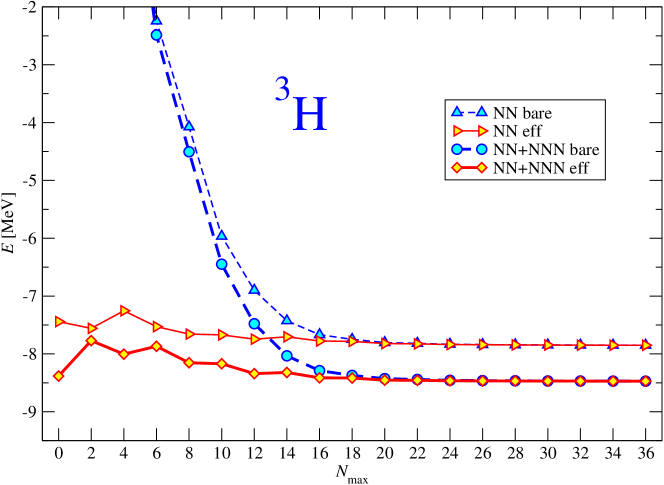
Figure 1: ³H ground-state energy dependence on the size of the basis. The HO frequency of $\hbar\Omega=28$ MeV was employed. Results with (thick lines) and without (thin lines) the NNN interaction are shown. The full lines correspond to calculations with two-body effective interaction derived from the chiral NN interaction, the dashed lines to calculations with the bare chiral NN interaction.

In Fig. 2, we show convergence of the ⁴He ground-state energy. The NCSM calculations are performed in basis spaces up to $N_{\rm max}=20$. Thin lines correspond to results obtained with the NN interaction only, while thick lines correspond to calculations that also include the NNN interaction. The dashed lines correspond to results obtained with bare interactions. The full lines correspond to results obtained using three-body effective interaction (the NCSM three-body cluster approximation). It is apparent that the use of the three-body effective interaction improves the convergence rate dramatically. We can see that at about $N_{\rm max}=18$ the bare interaction calculation reaches convergence as well. It should be noted, however, that $p$-shell calculations with the NNN interactions are presently feasible in model spaces up to $N_{\rm max}=6$ or $N_{\max}=8$. The use of the three-body effective interaction is then essential in the $p$-shell calculations. The calculation without NNN interaction was done for two different HO frequencies. it is apparent that convergence to the same result is in both cases. We note that in the case of no NNN interaction, we may use just the two-body effective interaction (two-body cluster approximation), which is much simpler. The convergence is slower, however, see discussion in Ref. [27]. We also note that ⁴He properties with the chiral EFT NN interaction that we employ here were calculated using two-body cluster approximation in Ref. [28] and present results are in agreement with results found there. Our ⁴He results ground state energy results are $-25.39(1)$ MeV in the NN case and $-28.34(2)$ MeV in the NN+NNN case. The experimental value is $-28.296$ MeV. We note that the present ab initio NCSM ³H and ⁴He results obtained with the chiral EFT NN interaction are in a perfect agreement with results obtained using the variational calculations in the hyperspherical harmonics basis as well as with the Faddeev-Yakubovsky calculations published in Ref. [29]. A satisfying feature of the present NCSM calculation is the fact that the rate of convergence is not affected in any significant way by inclusion of the NNN interaction.

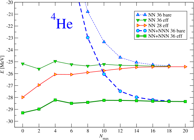
Figure 2: ⁴He ground-state energy dependence on the size of the basis. The HO frequencies of $\hbar\Omega=28$ and 36 MeV was employed. Results with (thick lines) and without (thin lines) the NNN interaction are shown. The full lines correspond to calculations with three-body effective interaction, the dashed lines to calculations with the bare interaction. For further details see the text.

As yet another example of convergence of ab initio NCSM calculations, we present the excitation energy calculations of the five lowest excited states of ⁶Li using the chiral EFT NN potential. The NCSM excitation energy dependence on the basis size is presented in Fig. 3 for the HO frequency of $\hbar\Omega=12$ MeV. Due to the complexity of the calculations, the lowest four state were obtained in basis spaces up to $N_{\rm max}=14$ while we stopped at $N_{\rm max}=12$ for the $2^{+}1$ and the $1^{+}_{2}0$ state. The calculations were performed using the two-body effective interaction in the Slater determinant HO basis with the shell model code Antoine [30]. Results for other HO frequencies were published in Ref. [28]. We observe that the convergence rate with $N_{\rm max}$ is different for different states. In particular, the $3^{+}0$ state and the $0^{+}1$ state converge faster in the higher frequency calculations ($\hbar\Omega=12,13$ MeV), while the higher lying states converge faster in the lower frequency calculations ($\hbar\Omega=8,10$ MeV). The results in Fig. 3 demonstrate a good convergence of the excitation energies in particular for the $3^{+}0$ and $0^{+}1$ states. An interesting results is the overestimation of the $3^{+}0$ excitation energy compared to experiment. It turns out that this problem is resolved once the NNN interaction is included in the Hamiltonian.

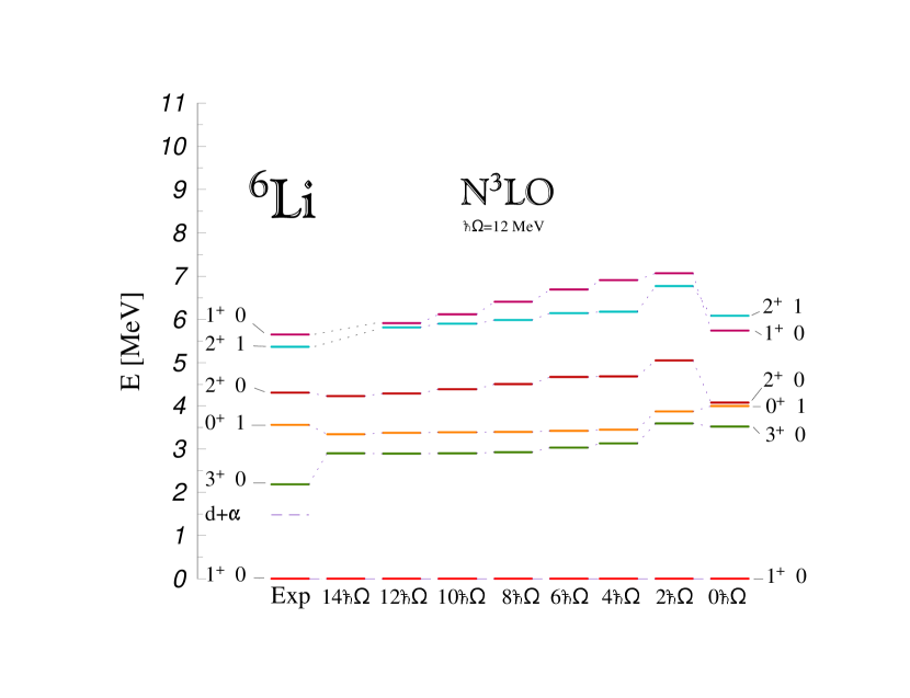
Figure 3: Calculated positive-parity excitation spectra of ⁶Li obtained in $0\hbar\Omega$-$14\hbar\Omega$ basis spaces using two-body effective interactions derived from the chiral EFT NN potential are compared to experiment. The HO frequency of $\hbar\Omega=12$ MeV was used.

3 Light nuclei from chiral EFT interactions

Interactions among nucleons are governed by quantum chromodynamics (QCD). In the low-energy regime relevant to nuclear structure, QCD is non-perturbative, and, therefore, hard to solve. Thus, theory has been forced to resort to models for the interaction, which have limited physical basis. New theoretical developments, however, allow us connect QCD with low-energy nuclear physics. The chiral effective field theory ($\chi$EFT) [31] provides a promising bridge. Beginning with the pionic or the nucleon-pion system [32] one works consistently with systems of increasing nucleon number [33, 34, 35]. One makes use of spontaneous breaking of chiral symmetry to systematically expand the strong interaction in terms of a generic small momentum and takes the explicit breaking of chiral symmetry into account by expanding in the pion mass. Thereby, the NN interaction, the NNN interaction and also $\pi$N scattering are related to each other. The $\chi$EFT predicts, along with the NN interaction at the leading order, an NNN interaction at the 3rd order (next-to-next-to-leading order or N²LO) [31, 36, 37], and even an NNNN interaction at the 4th order (N³LO) [38]. The details of QCD dynamics are contained in parameters, low-energy constants (LECs), not fixed by the symmetry. These parameters can be constrained by experiment. At present, high-quality NN potentials have been determined at order N³LO [26]. A crucial feature of $\chi$EFT is the consistency between the NN, NNN and NNNN parts. As a consequence, at N²LO and N³LO, except for two LECs, assigned to two NNN diagrams, the potential is fully constrained by the parameters defining the NN interaction.

We adopt the potentials of the $\chi$EFT at the orders presently available, the NN at N³LO of Ref. [26] and the NNN interaction at N²LO [36, 37]. Since the NN interaction is non-local, the ab initio NCSM is the only approach currently available to solve the resulting many-body Schrödinger equation for mid-$p$-shell nuclei. We are in a position to use the ab initio NCSM calculations in two ways. One of them is the determination of the LECs assigned to two NNN diagrams that must be determined in $A\geq 3$ systems. The other is testing predictions of the chiral NN and NNN interactions for light nuclei.

The NNN interaction at N²LO of the $\chi$EFT comprises of three parts: (i) The two-pion exchange, (ii) the one-pion exchange plus contact and the three-nucleon contact, see Fig. 4. The LECs associated with the two-pion exchange also appear in the NN interaction and are therefore determined in the $A=2$ system. The one-pion exchange plus contact term (D-term) is associated with the LEC $c_{D}$ and the three-nucleon contact term (E-term) is associated with the LEC $c_{E}$. The $c_{D}$ and $c_{E}$ LECs, expected to be of order one, can be constrained by the $A=3$ binding energy. We then still need additional observable to determine the two parameters. Their determination from three-nucleon scattering data is difficult due to a correlation of the ³H binding energy and, e.g. the $nd$ doublet scattering length [37] and, in general, due to the lack of an in-depth three-nucleon scattering phase shift analysis. We therefore investigate sensitivity of the $A>3$ nuclei properties to the variation of the constrained LECs.

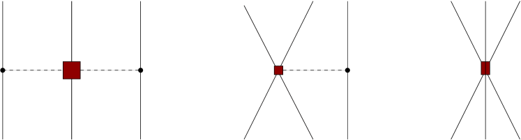
Figure 4: Terms of the N²LO $\chi$EFT NNN interaction.

Before presenting results of the ab initio NCSM calculations with the $\chi$EFT NN+NNN interactions, most of which were published in Ref. [39], let us discuss briefly a few technical details of the calculations with the NNN interaction. The NNN interaction is symmetric under permutation of the three nucleon indexes. It can be written as a sum of three pieces related by particle permutations:

$$W=W_{1}+W_{2}+W_{3}$$ (46)

To obtain its matrix element in an antisymmetrized three-nucleon basis we need to consider just a single term, e.g. $W_{1}$. Using the basis introduced in Eq. (27), a general matrix element can be written as

$$\langle NiJT|W|N^{\prime}i^{\prime}JT\rangle = 3\langle NiJT|W_{1}|N^{\prime}i^{\prime}JT\rangle$$ (47)

$$= 3\sum\langle nlsjt,{\cal NLJ}||NiJT\rangle\langle n^{\prime}l^{\prime}s^{\prime}j^{\prime}t^{\prime},{\cal N^{\prime}L^{\prime}J^{\prime}}||N^{\prime}i^{\prime}JT\rangle$$

$$\times\langle(nlsjt,{\cal NLJ})JT|W_{1}|(n^{\prime}l^{\prime}s^{\prime}j^{\prime}t^{\prime},{\cal N^{\prime}L^{\prime}J^{\prime}})JT\rangle\;.$$

We consider just the most trivial part of the $\chi$EFT N²LO NNN interaction, the three-nucleon contact term and evaluate its matrix element to demonstrate that non-trivial effort is needed to include the NNN interactions in many-body calculations. The three-nucleon contact term can be written as

$$W_{1}^{\rm cont} = E\vec{\tau}_{2}\cdot\vec{\tau}_{3}\delta(\vec{r}_{1}-\vec{r}_{2})\delta(\vec{r}_{3}-\vec{r}_{1})$$ (48)

$$= E\vec{\tau}_{2}\cdot\vec{\tau}_{3}\frac{1}{(2\pi)^{6}}\frac{1}{(\sqrt{3})^{3}}\int{\rm d}\vec{\pi}_{1}{\rm d}\vec{\pi}_{2}{\rm d}\vec{\pi}_{1}^{\prime}{\rm d}\vec{\pi}_{2}^{\prime}|\vec{\pi}_{1}\vec{\pi}_{2}\rangle\langle\vec{\pi}_{1}^{\prime}\vec{\pi}_{2}^{\prime}|\;,$$

with $E=\frac{c_{E}}{F_{\pi}^{4}\Lambda_{\chi}}$ where $\Lambda_{\chi}$ is the chiral symmetry breaking scale of the order of the $\rho$ meson mass and $F_{\pi}=92.4$ MeV is the weak pion decay constant. The $\vec{\pi}_{1}$ and $\vec{\pi}_{2}$ are Jacobi momenta associated with the the Jacobi coordinates $\vec{\xi}_{1}$ and $\vec{\xi}_{2}$ defined in Eq. (8) and (9).

The contact term must be regulated before it can be used in many-body calculations. We consider a regulator depending on momentum transfer:

$$W_{1}^{\rm cont,Q} = E\vec{\tau}_{2}\cdot\vec{\tau}_{3}\frac{1}{(2\pi)^{6}}\frac{1}{(\sqrt{3})^{3}}\int{\rm d}\vec{\pi}_{1}{\rm d}\vec{\pi}_{2}{\rm d}\vec{\pi}_{1}^{\prime}{\rm d}\vec{\pi}_{2}^{\prime}|\vec{\pi}_{1}\vec{\pi}_{2}\rangle F(\vec{Q}^{2};\Lambda)F(\vec{Q}^{\prime 2};\Lambda)\langle\vec{\pi}_{1}^{\prime}\vec{\pi}_{2}^{\prime}|$$ (49)

$$= E\vec{\tau}_{2}\cdot\vec{\tau}_{3}\int{\rm d}\vec{\xi}_{1}{\rm d}\vec{\xi}_{2}|\vec{\xi}_{1}\vec{\xi}_{2}\rangle Z_{0}(\textstyle{\sqrt{2}}\xi_{1};\Lambda)Z_{0}(|\textstyle{\frac{1}{\sqrt{2}}}\vec{\xi}_{1}+\textstyle{\sqrt{\frac{3}{2}}}\vec{\xi}_{2}|;\Lambda)\langle\vec{\xi}_{1}\vec{\xi}_{2}|\;,$$

with the regulator function $F(q^{2};\Lambda)=\exp(-q^{4}/\Lambda^{4})$. We defined momenta transferred by nucleon 2 and nucleon 3: $\vec{Q}=\vec{p}_{2}^{\prime}-\vec{p}_{2}=-\frac{1}{\sqrt{2}}(\vec{\pi}_{1}^{\prime}-\vec{\pi}_{1})+\frac{1}{\sqrt{6}}(\vec{\pi}_{2}^{\prime}-\vec{\pi}_{2})$ and $\vec{Q}^{\prime}=\vec{p}_{3}^{\prime}-\vec{p}_{3}=-\sqrt{\frac{2}{3}}(\vec{\pi}_{2}^{\prime}-\vec{\pi}_{2})$. Also, we introduced the function

$$Z_{0}(r;\Lambda)=\frac{1}{2\pi^{2}}\int{\rm d}qq^{2}j_{0}(qr)F(q^{2};\Lambda)\;.$$ (50)

This results in an interaction local in coordinate space because of the dependence of the regulator function on differences of initial and final Jacobi momenta. We can see that after the regulation, the form of the contact interaction becomes much more complicated. The three-nucleon matrix element of the regulated term is then obtained in the form

$$\langle(nlsjt,{\cal NLJ})JT|W_{1}^{\rm cont,Q}|(n^{\prime}l^{\prime}s^{\prime}j^{\prime}t^{\prime},{\cal N^{\prime}L^{\prime}J^{\prime}})JT\rangle$$ (63)

$$= E6\delta_{ss^{\prime}}\hat{t}\hat{t}^{\prime}(-1)^{t+t^{\prime}+T+\textstyle{\frac{1}{2}}}\left\{\begin{array}[]{ccc}t&t^{\prime}&1\\ \textstyle{\frac{1}{2}}&\textstyle{\frac{1}{2}}&\textstyle{\frac{1}{2}}\end{array}\right\}\left\{\begin{array}[]{ccc}t&t^{\prime}&1\\ \textstyle{\frac{1}{2}}&\textstyle{\frac{1}{2}}&T\end{array}\right\}$$

$$\times\hat{j}\hat{j}^{\prime}\hat{\cal J}\hat{\cal J}^{\prime}\hat{l}^{\prime}\hat{\cal L}^{\prime}(-1)^{J-\textstyle{\frac{1}{2}}+{\cal J}^{\prime}-{\cal J}+l+{\cal L}+s}$$

$$\times\sum_{X}(-1)^{X}\hat{X}^{2}\left\{\begin{array}[]{ccc}l^{\prime}&l&X\\ j&j^{\prime}&s\end{array}\right\}\left\{\begin{array}[]{ccc}j&j^{\prime}&X\\ {\cal J}^{\prime}&{\cal J}&J\end{array}\right\}\left\{\begin{array}[]{ccc}{\cal J}^{\prime}&{\cal J}&X\\ {\cal L}&{\cal L}^{\prime}&\textstyle{\frac{1}{2}}\end{array}\right\}$$

$$\times(l^{\prime}0X0|l0)({\cal L}^{\prime}0X0|{\cal L}0)$$

$$\times\int{\rm d}\xi_{1}{\rm d}\xi_{2}\xi_{1}^{2}\xi_{2}^{2}R_{nl}(\xi_{1},\textstyle{b})R_{{\cal N}{\cal L}}(\xi_{2},\textstyle{b})R_{n^{\prime}l^{\prime}}(\xi_{1},\textstyle{b})R_{{\cal N}^{\prime}{\cal L}^{\prime}}(\xi_{2},\textstyle{b})$$

$$\times Z_{0}(\textstyle{\sqrt{2}}\xi_{1};\Lambda)Z_{0,X}(\sqrt{\textstyle{\frac{1}{2}}}\xi_{1},\sqrt{\textstyle{\frac{3}{2}}}\xi_{2};\Lambda)\;,$$

with a new function

$$Z_{0,X}(r_{1},r_{2};\Lambda)=\frac{1}{2\pi^{2}}\int{\rm d}qq^{2}j_{X}(qr_{1})j_{X}(qr_{2})F(q^{2};\Lambda)\;.$$ (64)

and customary abbreviation $\hat{l}=\sqrt{2l+1}$. Evaluation of the other N²LO NNN terms is still more complicated.

It is important to note that our NCSM results through $A=4$ are fully converged in that they are independent of the $N_{\rm max}$ cutoff and the $\hbar\Omega$ HO energy. This was demonstrated in the subsection on the ab initio NCSM convergence tests in particular for the chiral EFT interactions we are investigating here. For heavier systems, we characterize the approach to convergence by the dependence of results on $N_{\rm max}$ and $\hbar\Omega$.

Fig. 5 shows the trajectories of the two LECs $c_{D}-c_{E}$ that are determined from fitting the binding energies of the $A=3$ systems. Separate curves are shown for ³H and ³He fits, as well as their average. There are two points where the binding of ⁴He is reproduced exactly. We observe, however, that in the whole investigated range of $c_{D}-c_{E}$, the calculated ⁴He binding energy is within a few hundred keV of experiment. Consequently, the determination of the LECs in this way is likely not very stringent. We therefore investigate the sensitivity of the $p$-shell nuclear properties to the choice of the $c_{D}-c_{E}$ LECs. First, we maintain the $A=3$ binding energy constraint. Second, we limit ourselves to the $c_{D}$ values in the vicinity of the point $c_{D}\sim 1$ since the values close to the point $c_{D}\sim 10$ overestimate the ⁴He radius. Also this large value might be considered “unnatural” from the $\chi$EFT point of view.

Figure 5: Relations between $c_{D}$ and $c_{E}$ for which the binding energy of ³H ($8.482$ MeV) and ³He ($7.718$ MeV) are reproduced. (a) ⁴He ground-state energy along the averaged curve. (b) ⁴He charge radius $r_{c}$ along the averaged curve. Dotted lines represent the $r_{c}$ uncertainty due to the uncertainties in the proton charge radius.

While most of the $p$-shell nuclear properties, e.g. excitation spectra, are not very sensitive to variations of $c_{D}$ in the vicinity of the $c_{D}\sim 1$ point, we were able to identify several observables that do demonstrate strong dependence on $c_{D}$. For example, the ⁶Li quadrupole moment that changes sign depending on the choice of $c_{D}$. In Fig. 6, we display the ratio of the B(E2) transitions from the ¹⁰B ground state to the first and the second $1^{+}0$ state. This ratio changes by several orders of magnitude depending on the $c_{D}$ variation. This is due to the fact that the structure of the two $1^{+}0$ states is exchanged depending on $c_{D}$.

Figure 6: Dependence on the $c_{D}$ with the $c_{E}$ constrained by the $A=3$ binding energy fit for different basis sizes for ¹⁰B B(E2;$3^{+}_{1}0\rightarrow 1^{+}_{1}0$)/B(E2;$3^{+}_{1}0\rightarrow 1^{+}_{2}0$) ratio. The HO frequency of $\hbar\Omega=14$ MeV was employed.

In Fig. 7, we present the ¹²C B(M1) transition from the ground state to the $1^{+}1$ state. The B(M1) transition inset illustrates the importance of the NNN interaction in reproducing the experimental value [40]. Overall our results show that for $c_{D}<-2$ the ⁴He radius and the ⁶Li quadrupole moment underestimate experiment while for $c_{D}>0$ the lowest two $1^{+}$ states of ¹⁰B are reversed and the ¹²C B(M1;$0^{+}0\rightarrow 1^{+}1$) is overestimated. We therefore select $c_{D}=-1$ as globally the best choice and use it for our further investigation.

Figure 7: Dependence on the $c_{D}$ with the $c_{E}$ constrained by the $A=3$ binding energy fit for different basis sizes for the ¹²C B(M1;$0^{+}0\rightarrow 1^{+}1$). The HO frequency of $\hbar\Omega=15$ MeV was employed. In the inset, the convergence of the B(M1;$0^{+}0\rightarrow 1^{+}1$) is presented for calculations with (using $c_{D}=-1$) and without the NNN interaction.

We present in Figs. 8 and 9 the excitation spectra of ¹⁰B as a function of $N_{\rm max}$ for both the chiral NN+NNN, as well as with the chiral NN interaction alone. In both cases, the convergence with increasing $N_{\rm max}$ is quite quite reasonable for the low-lying states. Similar convergence rates are obtained for our other $p-$shell nuclei.

Figure 8: ¹⁰B excitation spectra as function of the basis space size $N_{\rm max}$ at $\hbar\Omega=15$ MeV using the chiral NN interaction and comparison with experiment. The isospin of the states not explicitly depicted is $T$=0.

A remarkable feature of the ¹⁰B results is the observation that the chiral NN interaction alone predicts incorrect ground-state spin of ¹⁰B. The experimental value is $3^{+}0$ while the calculated one is $1^{+}0$. On the other hand, once we also include the chiral NNN interaction in the Hamiltonian, which is actually required by the $\chi$EFT, the correct ground-state spin is predicted. Further, once we select the $c_{D}$ value as discussed above, i.e. $c_{D}=-1$, we also obtain the two lowest $1^{+}0$ states in the experimental order.

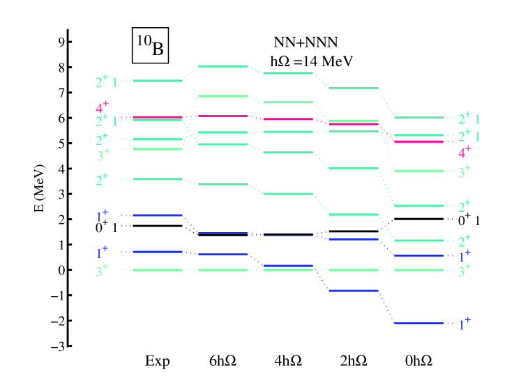
Figure 9: ¹⁰B excitation spectra as function of the basis space size $N_{\rm max}$ at $\hbar\Omega=14$ MeV using the chiral NN+NNN interaction and comparison with experiment. The isospin of the states not explicitly depicted is $T$=0.

We display in Fig. 10 the natural parity excitation spectra of four nuclei in the middle of the $p-$shell with both the NN and the NN+NNN effective interactions from $\chi$EFT. The results shown are obtained in the largest basis spaces achieved to date for these nuclei with the NNN interactions, $N_{\rm max}=6$ ($6\hbar\Omega$). Overall, the NNN interaction contributes significantly to improve theory in comparison with experiment. This is especially well-demonstrated in the odd mass nuclei for the lowest few excited states. The case of the ground state spin of ¹⁰B and its sensitivity to the presence of the NNN interaction discussed also in Figs. 8 and 9 is clearly evident. We note that the ¹⁰B results with the NN interaction only in Fig. 8 were obtained with the HO frequency of $\hbar\Omega=15$ MeV, while those in Fig. 10 with $\hbar\Omega=14$ MeV. A weak HO frequency dependence of the $N_{\rm max}=6$ results is evident. The ¹⁰B results with NN+NNN interaction presented in Figs. 9 and 10 were obtained using the same HO frequency. Still, one may notice small differences of the $N_{\rm max}=6$ results. The reason behind those differences is the use of two alternative D-term regularizations (both depending on the momentum transfer, details will be discussed elsewhere). As the dependence on the regulator is a higher order effect than the $\chi$EFT expansion order used to derive the NNN interaction, these differences should have only minor effect. It is satisfying that the present ¹⁰B results appear to support this expectation.

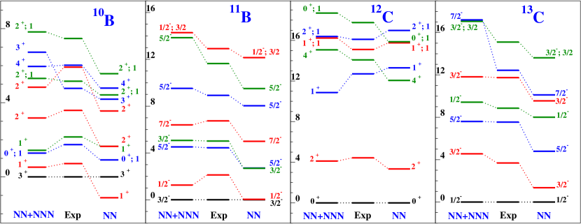
Figure 10: States dominated by $p$-shell configurations for ¹⁰B, ¹¹B, ¹²C, and ¹³C calculated at $N_{\rm max}=6$ using $\hbar\Omega=15$ MeV (14 MeV for ¹⁰B). Most of the eigenstates are isospin $T$=0 or 1/2, the isospin label is explicitly shown only for states with $T$=1 or 3/2. The excitation energy scales are in MeV.

Concerning the ¹²C results, there is an initial indication that the chiral NNN interaction is somewhat over-correcting the inadequacies of the NN interaction since, e.g. $1^{+}0$ and the $4^{+}0$ states in ¹²C are not only interchanged but they are also spread apart more than the experimentally observed separation. In the ¹³C results, we can also identify an indication of an overly strong correction arising from the chiral NNN interaction as seen in the upward shift of the $\frac{7}{2}^{-}$ state. However, the experimental $\frac{7}{2}^{-}$ may have significant intruder components and is not well-matched with our state. In addition, convergence for some higher lying states is affected by incomplete treatment of clustering in the NCSM. This point will be elaborated upon later. These results required substantial computer resources. A typical $N_{\rm max}=6$ spectrum shown in Fig. 10 and a set of additional experimental observables, takes 4 hours on 3500 processors of the LLNL’s Thunder machine. The $A$-nucleon calculations were performed in the Slater determinant HO basis using the shell model code MFD [41]. More details on some of the results discussed here are published Ref. [39].

The calculations presented in this section demonstrate that the chiral NNN interaction makes substantial contributions to improving the spectra and other observables. However, there is room for further improvement in comparison with experiment. In these calculations we used a strength of the 2$\pi$-exchange piece of the NNN interaction, which is consistent with the NN interaction that we employed (i.e. from Ref. [26]). This strength is somewhat uncertain (see e.g. Ref. [24]). Therefore, it will be important to study the sensitivity of our results with respect to this strength. Further on, it will be interesting to incorporate sub-leading NNN interactions and also four-nucleon interactions, which are also order N³LO [38]. Finally, it will be useful to extend the basis spaces to $N_{\rm max}=8$ ($8\hbar\Omega$) for $A>6$ to further improve convergence.

4 Cluster overlap functions and S-factors of capture reactions

In the ab initio NCSM calculations, we are able to obtain wave functions of low-lying states of light nuclei in large model spaces. An interesting and important question is, what is the cluster structure of these wave functions. That is we want to understand, how much, e.g. an ⁶Li eigenstate looks like ⁴He plus deuteron, an ⁷Be eigenstate looks like ⁴He plus ³He, an ⁸B eigenstate looks like ⁷Be plus proton and so on. This information is important for the description of low-energy nuclear reactions. To gain insight, one introduces channel cluster form factors (or overlap integrals, overlap functions). The formalism for calculating the channel cluster form factors from the NCSM wave functions was developed in Ref. [42]. Here we just briefly repeat a part of the formalism relevant to the simplest case when the lighter of the two clusters is a single-nucleon.

We consider a composite system of $A$ nucleons, i.e. ⁸B, a nucleon projectile, here a proton, and an $A-1$-nucleon target, i.e. ⁷Be. Both nuclei are assumed to be described by eigenstates of the NCSM effective Hamiltonians expanded in the HO basis with identical HO frequency and the same (for the eigenstates of the same parity) or differing by one unit of the HO excitation (for the eigenstates of opposite parity) definitions of the model space. The target and the composite system is assumed to be described by wave functions expanded in Slater determinant single-particle HO basis (that is obtained from a calculation using a shell model code like Antoine).

Let us introduce a projectile-target wave function

$$\langle\vec{\xi}_{1}\ldots\vec{\xi}_{A-2}r^{\prime}\hat{r}|\Phi_{(l\frac{1}{2})j;\alpha I_{1}}^{(A-1,1)JM};\delta_{r}\rangle = \sum(jmI_{1}M_{1}|JM)(lm_{l}\textstyle{\frac{1}{2}}m_{s}|jm)\frac{\delta(r-r^{\prime})}{rr^{\prime}}$$ (65)

$$\times Y_{lm_{l}}(\hat{r})\chi_{m_{s}}\langle\vec{\xi}_{1}\ldots\vec{\xi}_{A-2}|A-1\alpha I_{1}M_{1}\rangle\;,$$

where $\langle\vec{\xi}_{1}\ldots\vec{\xi}_{A-2}|A-1\alpha I_{1}M_{1}\rangle$ and $\chi_{m_{s}}$ are the target and the nucleon wave function, respectively. Here, $l$ is the channel relative orbital angular momentum, $\vec{\xi}$ are the target Jacobi coordinates defined in Eq. (7) and $\vec{r}=\left[\frac{1}{A-1}\left(\vec{r}_{1}+\vec{r}_{2}+\ldots+\vec{r}_{A-1}\right)-\vec{r}_{A}\right]$ describes the relative distance between the nucleon and the center of mass of the target. The spin and isospin coordinates were omitted for simplicity.

The channel cluster form factor is then defined by

$$g^{A\lambda J}_{(l\frac{1}{2})j;A-1\alpha I_{1}}(r)=\langle A\lambda J|{\cal A}\Phi_{(l\frac{1}{2})j;\alpha I_{1}}^{(A-1,1)J};\delta_{r}\rangle\;,$$ (66)

with ${\cal A}$ the antisymmetrizer and $|A\lambda J\rangle$ an eigenstate of the $A$-nucleon composite system (here ⁸B). It can be calculated from the NCSM eigenstates obtained in the Slater-determinant basis from a reduced matrix element of the creation operator. The derivation is as follows. First, we use the relation (29) for both the composite $A$-nucleon and the target $A-1$-nucleon eigenstate. With the help of relations analogous to (6):

$$\sum_{Mm}(LMlm|Qq)\varphi_{NLM}(\vec{R}^{A-1}_{\rm CM})\varphi_{nlm}(\vec{r}_{A})=$$

$$\sum_{n^{\prime}l^{\prime}m^{\prime}N^{\prime}L^{\prime}M^{\prime}}\langle n^{\prime}l^{\prime}N^{\prime}L^{\prime}Q|NLnlQ\rangle_{\frac{1}{A-1}}(l^{\prime}m^{\prime}L^{\prime}M^{\prime}|Qq)\varphi_{n^{\prime}l^{\prime}m^{\prime}}(\vec{\xi}_{A-1})\varphi_{N^{\prime}L^{\prime}M^{\prime}}(\vec{\xi}_{0})\;,$$ (67)

we obtain

$$_{\rm SD}\langle A\lambda J|{\cal A}\Phi_{(l\frac{1}{2})j;\alpha I_{1}}^{(A-1,1)J};nl\rangle_{\rm SD}\;=\langle nl00l|00nll\rangle_{\frac{1}{A-1}}\;\langle A\lambda J|{\cal A}\Phi_{(l\frac{1}{2})j;\alpha I_{1}}^{(A-1,1)J};nl\rangle\;,$$ (68)

with a general HO bracket due to the CM motion. The $nl$ in (68) refers to a replacement of $\delta_{r}$ by the HO $R_{nl}(r)$ radial wave function. Second, we relate the SD overlap to a linear combination of matrix elements of a creation operator between the target and the composite eigenstates ${}_{\rm SD}\langle A\lambda J|a^{\dagger}_{nlj}|A-1\alpha I_{1}\rangle_{\rm SD}$. The subscript SD refers to the fact that these states were obtained in the Slater determinant basis. Such matrix elements are easily calculated by shell model codes. The result is

$$\langle A\lambda J|{\cal A}\Phi_{(l\textstyle{\frac{1}{2}},j);\alpha I_{1}}^{(A-1,1)J};\delta_{r}\rangle = \sum_{n}R_{nl}(r)\frac{1}{\langle nl00l|00nll\rangle_{\frac{1}{A-1}}}\frac{1}{\hat{J}}(-1)^{I_{1}-J-j}$$ (69)

$$\times\;_{\rm SD}\langle A\lambda J||a^{\dagger}_{nlj}||A-1\alpha I_{1}\rangle_{\rm SD}\;\;.$$

The eigenstates expanded in the Slater determinant basis contain CM components. A general HO bracket, which value is simply given by

$$\langle nl00l|00nll\rangle_{\frac{1}{A-1}}=(-1)^{l}\left(\frac{A-1}{A}\right)^{\frac{2n+l}{2}}\;,$$ (70)

then appears in Eq. (69) in order to remove these components. The $R_{nl}(r)$ in Eq. (69) is the radial HO wave function with the oscillator length parameter $b=\sqrt{\frac{\hbar}{\frac{A-1}{A}m\Omega}}$, where $m$ is the nucleon mass.

A conventional spectroscopic factor is obtained by integrating the square of the cluster form factor:

$$S^{A\lambda J}_{(l\frac{1}{2})j;A-1\alpha I_{1}}=\int drr^{2}|g^{A\lambda J}_{(l\frac{1}{2})j;A-1\alpha I_{1}}(r)|^{2}\;.$$ (71)

A generalization for projectiles (= the lighter of the two clusters) with 2, 3 or 4 nucleons is straightforward, although the expressions become more involved. In all cases, the projectile is described by wave function expanded in Jacobi coordinate HO basis, while the composite and the target eigenstates are expanded in the Slater determinant HO basis. Full details are given in Ref. [42].

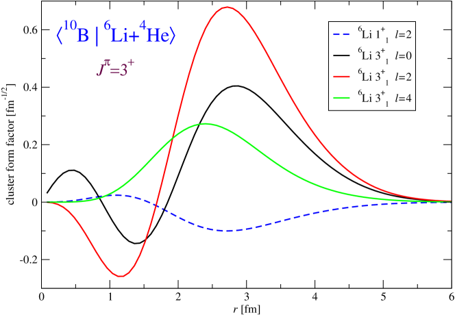
Figure 11: Overlap integral of ¹⁰B ground state with ⁶Li+⁴He as a function of separation between the ⁴He and the⁶Li. Results for the ⁶Li $1^{+}0$ ground state and the first excited $3^{+}0$ state are compared. The $\chi$EFT NN+NNN interaction and the $N_{max=6}$ model space for ¹⁰B and ⁶Li were used.

As an example, in Fig. 11 we present the cluster overlap function of ¹⁰B ground state with ⁶Li+⁴He. Results are given for ⁶Li in the $1^{+}0$ ground state and in the $3^{+}0$ excited state. We can see that the ⁶Li $1^{+}0$ ground-state component is rather small. The ¹⁰B ground state is dominated by a superposition of $S$-, $D$- and $G$-waves of relative motion of ⁴He and ⁶Li in the $3^{+}0$ state.

The overlap functions introduced in this subsection are relevant for description of low-energy $\gamma$-capture reactions important for nuclear astrophysics. Next, we investigate three reactions of this type.

4.1 ⁷Be(p,$\gamma$)⁸B

The ⁷Be(p,$\gamma$)⁸B capture reaction serves as an important input for understanding the solar neutrino flux [43]. Recent experiments have determined the neutrino flux emitted from ⁸B with a precision of  9% [44]. On the other hand, theoretical predictions have uncertainties of the order of 20% [45, 46]. The theoretical neutrino flux depends on the ⁷Be(p,$\gamma$)⁸B S-factor. Many experimental and theoretical investigations studied this reaction.

In this subsection, we discuss a calculation of the ⁷Be(p,$\gamma$)⁸B S-factor starting from ab initio wave functions of ⁸B and ⁷Be. It should be noted that the aim of ab initio approaches is to predict correctly absolute cross sections (S-factors), not only relative cross sections. The full details of our ⁷Be(p,$\gamma$)⁸B investigation were published in Refs. [47, 48].

Our calculations for both ⁷Be and ⁸B nuclei were performed using the high-precision CD-Bonn 2000 NN potential [49] in model spaces up to $10\hbar\Omega$ ($N_{\rm max}=10$) for a wide range of HO frequencies. From the obtained ⁸B and ⁷Be wave functions, we calculate the channel cluster form factors (overlap functions, overlap integrals) $g^{A\lambda J}_{(l\frac{1}{2})j;A-1\alpha I_{1}}(r)$ as discussed in the previous subsection. Here, $A=8$, $l$ is the channel relative orbital angular momentum and $\vec{r}=\left[\frac{1}{A-1}\left(\vec{r}_{1}+\vec{r}_{2}+\ldots+\vec{r}_{A-1}\right)-\vec{r}_{A}\right]$ describes the relative distance between the proton and the center of mass of ⁷Be. The two most important channels are the $p$-waves, $l=1$, with the proton in the $j=3/2$ and $j=1/2$ states, $\vec{j}=\vec{l}+\vec{s},s=1/2$. In these channels, we obtain the spectroscopic factors of $0.96$ and $0.10$, respectively. The dominant $j=3/2$ overlap integral is presented in Fig. 12 by the full line. The $10\hbar\Omega$ model space and the HO frequency of $\hbar\Omega=12$ MeV were used. Despite the fact, that a very large basis was employed in the present calculation, it is apparent that the overlap function is nearly zero at about 10 fm. This is a consequence of the HO basis asymptotic behavior. As already discussed, in the ab initio NCSM, the short-range correlations are taken into account by means of the effective interaction. The medium-range correlations are then included by using a large, multi-$\hbar\Omega$ HO basis. The long-range behavior is not treated correctly, however. The proton capture on ⁷Be to the weakly bound ground state of ⁸B associated dominantly by the $E1$ radiation is a peripheral process. In order to calculate the S-factor of this process we need to go beyond the ab initio NCSM as done up to this point. We expect, however, that the interior part of the overlap function is realistic. It is then straightforward to find a quick fix and correct the asymptotic behavior of the overlap functions, which should be proportional to the Whittaker function.

One possibility we explored utilizes solutions of a Woods-Saxon (WS) potential. In particular, we performed a least-square fit of a WS potential solution to the interior of the NCSM overlap in the range of $0-4$ fm. The WS potential parameters were varied in the fit under the constraint that the experimental separation energy of ⁷Be+p, $E_{0}=0.137$ MeV, was reproduced. In this way we obtain a perfect fit to the interior of the overlap integral and a correct asymptotic behavior at the same time. The result is shown in Fig. 12 by the dashed line.

Another possibility is a direct matching of logarithmic derivatives of the NCSM overlap integral and the Whittaker function: $\frac{d}{dr}ln(rg_{lj}(r))=\frac{d}{dr}ln(C_{lj}W_{-\eta,l+1/2}(2k_{0}r))$, where $\eta$ is the Sommerfeld parameter, $k_{0}=\sqrt{2\mu E_{0}}/\hbar$ with $\mu$ the reduced mass and $E_{0}$ the separation energy. Since asymptotic normalization constant (ANC) $C_{lj}$ cancels out, there is a unique solution at $r=R_{m}$. For the discussed overlap presented in Fig. 12, we found $R_{m}=4.05$ fm. The corrected overlap using the Whittaker function matching is shown in Fig. 12 by a dotted line. In general, we observe that the approach using the WS fit leads to deviations from the original NCSM overlap starting at a smaller radius. In addition, the WS solution fit introduces an intermediate range from about 4 fm to about 6 fm, where the corrected overlap deviates from both the original NCSM overlap and the Whittaker function. Perhaps, this is a more realistic approach compared to the direct Whittaker function matching. In any case, by considering the two alternative procedures we are in a better position to estimate uncertainties in our S-factor results.

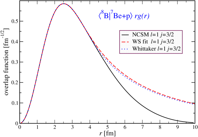
Figure 12: Overlap function, $rg(r)$, for the ground state of ⁸B with the ground state of ⁷Be plus proton as a dependence on separation between the ⁷Be and the proton. The $p$-wave channel with $j=3/2$ is shown. The full line represents the NCSM result obtained using the CD-Bonn 2000 NN potential, the $10\hbar\Omega$ model space and the HO frequency of $\hbar\Omega=12$ MeV. The dashed lines represent corrected overlaps obtained from a Woods-Saxon potential whose parameters were fit to the NCSM overlaps up to  4.0 fm under the constraint to reproduce the experimental separation energy. The dotted lines represent overlap corrections by the direct Whittaker function matching.

In the end, we re-scale the corrected overlap functions to preserve the original NCSM spectroscopic factors (Table 2 of Ref. [47]). In general, we observe a faster convergence of the spectroscopic factors than that of the overlap functions. The corrected overlap function should represent the infinite space result. By re-scaling a corrected overlap function obtained at a finite $N_{\rm max}$, we approach faster the infinite space result. At the same time, by re-scaling we preserve the spectroscopic factor sum rules.

The S-factor for the reaction ${}^{7}{\rm Be(p},\gamma)^{8}{\rm B}$ also depends on the continuum wave function, $R_{lj}^{(c)}$. As we have not yet developed an extension of the NCSM to describe continuum wave functions (see, however, the discussion in Sect. 5), we obtain $R_{lj}^{(c)}$ for $s$ and $d$ waves from a WS potential model. Since the largest part of the integrand stays outside the nuclear interior, one expects that the continuum wave functions are well described in this way. In order to have the same scattering wave function in all the calculations, we chose a WS potential from Ref. [50] that was fitted to reproduce the $p$-wave $1^{+}$ resonance in ⁸B. It was argued [51] that such a potential is also suitable for the description of $s$- and $d$-waves. We note that the S-factor is very weakly dependent on the choice of the scattering-state potential (using our fitted potential for the scattering state instead changes the S-factor by less than 1.5 eV b at 1.6 MeV with no change at 0 MeV).

Our obtained S-factor is presented in Figs. 13 where contribution from the two partial waves are shown together with the total result. It is interesting to note a good agreement of our calculated S-factor with the recent Seattle direct measurement [52].

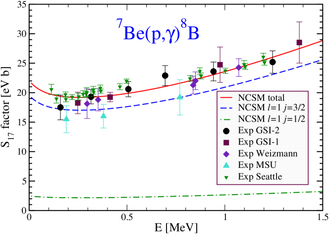
Figure 13: The ⁷Be(p,$\gamma$)⁸B S-factor obtained using the NCSM overlap functions with corrected asymptotics as described in the text. The dashed and dashed-dotted lines show the contribution due to the $l=1$, $j=3/2$ and $j=1/2$ partial waves, respectively. Experimental values are from Refs. [52, 53].

In order to judge the convergence of our S-factor calculation, we performed a detailed investigation of the model-space-size and the HO frequency dependencies. We used the HO frequencies in the range from $\hbar\Omega=11$ MeV to $\hbar\Omega=15$ MeV and the model spaces from $6\hbar\Omega$ to $10\hbar\Omega$. By analysing these results, we arrived at the S-factor value of $S_{17}(10\;{\rm keV})=22.1\pm 1.0$ eV b.

4.2 ³He($\alpha$,$\gamma$)⁷Be

The ³He($\alpha$,$\gamma$)⁷Be capture reaction cross section was identified the most important uncertainty in the solar model predictions of the neutrino fluxes in the p-p chain [46]. We investigated the bound states of ⁷Be, ³He and ⁴He within the ab initio NCSM and calculated the overlap functions of ⁷Be bound states with the ground states of ³He plus ⁴He as a function of separation between the ³He and the $\alpha$ particle. The obtained $p$-wave overlap functions of the ⁷Be $3/2^{-}$ ground state excited state are presented in Fig. 14 by the full line. The dashed lines show the corrected overlap function obtained by the least-square fits of the WS parameters done in the same way as in the ⁸B$\leftrightarrow^{7}$Be+p case. The corresponding NCSM spectroscopic factors obtained using the CD-Bonn 2000 in the $10\hbar\Omega$ model space for ⁷Be ($12\hbar\Omega$ for ^3,4He) and HO frequency of $\hbar\Omega=13$ MeV are 0.93 and 0.91 for the ground state and the first excited state of ⁷Be, respectively. We note that contrary to the ⁸B$\leftrightarrow^{7}$Be+p case, the ⁷Be$\leftrightarrow^{3}$He+$\alpha$ $p$-wave overlap functions have a node.

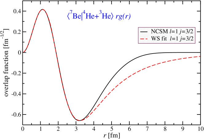
Figure 14: The overlap function, $rg(r)$, for the first excited state of ⁷Be with the ground state of ³He plus $\alpha$ as a dependence on separation between the ³He and the $\alpha$ particle. The $p$-wave channel overlap function with $j=3/2$ is shown. The full line represents the NCSM result obtained using the CD-Bonn 2000 NN potential and the $10\hbar\Omega$ model space for ⁷Be ($12\hbar\Omega$ for ^3,4He) with the HO frequency of $\hbar\Omega=13$ MeV. The dashed line represents a corrected overlap obtained with a Woods-Saxon potential whose parameters were fit to the NCSM overlap up to  3.4 fm under the constraint to reproduce the experimental separation energy.

Using the corrected overlap functions and a ³He+$\alpha$ scattering state obtained using the potential model of Ref. [54] we calculated the ³He($\alpha$,$\gamma$)⁷Be S-factor. Our $10\hbar\Omega$ result is presented in the left panel of Fig. 15. We show the total S-factor as well as the contributions from the capture to the ground state and the first excited state of ⁷Be. By investigating the model space dependence for $8\hbar\Omega$ and $10\hbar\Omega$ spaces we estimate the ³He($\alpha$,$\gamma$)⁷Be S-factor at zero energy to be higher than 0.44 keV b, the value that we obtained in the discussed case shown in Fig. 15. Our results are similar to those obtained by K. Nollett [55] using the variational Monte Carlo wave functions for the bound states and potential model wave functions for the scattering state.

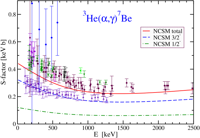
Figure 15: The full line shows the ³He($\alpha$,$\gamma$)⁷Be S-factor obtained using the NCSM overlap functions with corrected asymptotics. The dashed lines show the ⁷Be ground- and the first excited state contributions. The calculation was done using the CD-Bonn 2000 NN potential and the $10\hbar\Omega$ model space for ⁷Be ($12\hbar\Omega$ for ^3,4He) with the HO frequency of $\hbar\Omega=13$ MeV.

4.3 ³H($\alpha$,$\gamma$)⁷Li

An important check on the consistency of the ³He($\alpha$,$\gamma$)⁷Be S-factor calculation is the investigation of the mirror reaction ³H($\alpha$,$\gamma$)⁷Li, for which more accurate data exist [56]. Our results obtained using the CD-Bonn 2000 NN potential are shown in Fig. 16. It is apparent that our ³H($\alpha$,$\gamma$)⁷Li results are consistent with our ³He($\alpha$,$\gamma$)⁷Be calculation. We are on the lower side of the data and we find an increase of the S-factor as we increase the size of our basis.

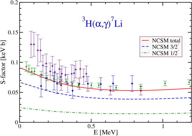
Figure 16: The full line shows the ³H($\alpha$,$\gamma$)⁷Li S-factor obtained using the NCSM overlap functions with corrected asymptotics. The dashed lines show the ⁷Li ground- and the first excited state contributions. The calculation was done using the CD-Bonn 2000 NN potential and the $10\hbar\Omega$ model space for ⁷Li ($12\hbar\Omega$ for ³H and ⁴He) with the HO frequency of $\hbar\Omega=13$ MeV.

More details on the ab initio NCSM investigation of the ³He($\alpha$,$\gamma$)⁷Be and ³H($\alpha$,$\gamma$)⁷Li S-factors are given in Ref. [57].

5 Towards the ab initio NCSM with continuum

In the previous section, we highlighted shortcomings of the ab initio NCSM, its incorrect description of long-range correlations and its lack of coupling to continuum. If we want to build upon the ab initio NCSM to microscopically describe loosely bound systems as well as nuclear reactions, the approach must be augmented by explicitly including cluster states such as, e.g. those given in Eq. (65), and solve for their relative motion while imposing the proper boundary conditions. This can be done by extending the ab initio NCSM HO basis through the addition of the cluster states. This would result in an over-complete basis with the cluster relative motion wave functions as amplitudes that need to be determined. The first step in this direction is to consider the cluster basis alone. This approach is very much in the spirit of the resonating group method (RGM) [58], a technique that considers clusters with fixed internal degrees of freedom, treats the Pauli principle exactly and solves the many-body problem by determining the relative motion between the various clusters. In our approach, we use the ab initio NCSM wave functions for the clusters involved and the ab initio NCSM effective interactions derived from realistic NN (and eventually also from NNN) potentials.

The general outline of the formalism is as follows. The many-body wave function is approximated by a superposition of binary cluster channel wave functions

$$\Psi^{(A)}=\sum_{\nu}\hat{\mathcal{A}}\left[\psi_{1\nu}^{(A-a)}\psi_{2\nu}^{(a)}\varphi_{\nu}(\vec{r}_{A-a,a})\right]=\sum_{\nu}\int d\vec{r}\,\varphi_{\nu}(\vec{r}\,)\,\hat{\mathcal{A}}\,\Phi_{\nu\vec{r}}^{(A-a,a)}\,,$$ (72)

with

$$\Phi_{\nu\vec{r}}^{(A-a,a)}=\psi_{1\nu}^{(A-a)}\psi_{2\nu}^{(a)}\delta(\vec{r}\,-\vec{r}_{A-a,a})\,.$$ (73)

Here, $\hat{\mathcal{A}}$ is the antisymmetrizer accounting for the exchanges of nucleons between the two clusters (which are already antisymmetric with respect to exchanges of internal nucleons). The relative-motion wave functions $\varphi_{\nu}$ depend on the relative-distance between the center of masses of the two clusters in channel $\nu$. They can be determined by solving the many-body Schrödinger equation in the Hilbert space spanned by the basis functions (73):

$$H\Psi^{(A)}=E\Psi^{(A)}\longrightarrow\,\sum_{\nu}\int d\vec{r}\,\left[{\mathcal{H}}^{(A-a,a)}_{\mu\nu}(\vec{r}\,^{\prime},\vec{r}\,)-E{\mathcal{N}}^{(A-a,a)}_{\mu\nu}(\vec{r}\,^{\prime},\vec{r}\,)\right]\varphi_{\nu}(\vec{r}\,)\,,$$ (74)

where the Hamiltonian and norm kernels are defined as

$${\mathcal{H}}^{(A-a,a)}_{\mu\nu}(\vec{r}\,^{\prime},\vec{r}\,) = \left\langle\Phi_{\mu\vec{r}\,^{\prime}}^{(A-a,a)}\left|\hat{\mathcal{A}}\,H\,\hat{\mathcal{A}}\right|\Phi_{\nu\vec{r}}^{(A-a,a)}\right\rangle\,,$$ (75)

$${\mathcal{N}}^{(A-a,a)}_{\mu\nu}(\vec{r}\,^{\prime},\vec{r}\,) = \left\langle\Phi_{\mu\vec{r}\,^{\prime}}^{(A-a,a)}\left|\hat{\mathcal{A}}^{2}\right|\Phi_{\nu\vec{r}}^{(A-a,a)}\right\rangle\,.$$ (76)

The most challenging task is to evaluate the Hamiltonian kernel and the norm kernel. We now briefly outline, how this is done when ab initio NCSM wave functions are used for the binary cluster states. From now on, let us consider the cluster states with a single-nucleon projectile ($a=1$ in Eq. 72). A generalization is straightforward. Using an alternative coupling scheme compared to Eq. (65), we introduce

$$\langle\vec{\xi}_{1}\ldots\vec{\xi}_{A-2}\xi_{A-1}^{\prime}\hat{\xi}_{A-1}|\Phi_{(\alpha I_{1}T_{1},\frac{1}{2}\frac{1}{2});sl}^{(A-1,1)JMTM_{T}};\delta_{\xi_{A-1}}\rangle$$ (77)

$$= \sum(I_{1}M_{1}\textstyle{\frac{1}{2}}m_{s}|sm)(smlm_{l}|JM)(T_{1}M_{T_{1}}\textstyle{\frac{1}{2}}m_{t}|TM_{T})\frac{\delta(\xi_{A-1}-\xi_{A-1}^{\prime})}{\xi_{A-1}\xi_{A-1}^{\prime}}$$

$$\times Y_{lm_{l}}(\hat{\xi}_{A-1})\chi_{m_{s}}\chi_{m_{t}}\langle\vec{\xi}_{1}\ldots\vec{\xi}_{A-2}|A-1\alpha I_{1}M_{1}T_{1}M_{T_{1}}\rangle\;,$$

with the spin and isospin coordinates omitted to simplify the notation. The Jacobi coordinates were defined in Eq. (7). Using the latter cluster basis and the following definition of the antisymmetrizer $\hat{\mathcal{A}}=1/\sqrt{A}(1-\sum_{j=1}^{A-1}P_{j,A})$ with $P_{j,A}$ the transposition operator of nucleons $j$ and $A$, the norm kernel can be expressed as

$${\mathcal{N}}^{(A-1,1)}_{\mu\nu}(r^{\prime},r) = \delta_{\mu\nu}\frac{\delta(r^{\prime}-r)}{r^{\prime}r}-(A-1)\sum_{n^{\prime}n}R_{n^{\prime}l^{\prime}}(r^{\prime})$$ (78)

$$\times \langle\Phi_{(\alpha^{\prime}I^{\prime}_{1}T^{\prime}_{1},\textstyle{\frac{1}{2}}\textstyle{\frac{1}{2}})s^{\prime}l^{\prime}}^{(A-1,1)JT};n^{\prime}l^{\prime}|P_{A,A-1}|\Phi_{(\alpha I_{1}T_{1},\textstyle{\frac{1}{2}}\textstyle{\frac{1}{2}})sl}^{(A-1,1)JT};nl\rangle R_{nl}(r)\;,$$

with $\mu\equiv(\alpha^{\prime}I^{\prime}_{1}T^{\prime}_{1},\textstyle{\frac{1}{2}}\textstyle{\frac{1}{2}})s^{\prime}$, $\nu\equiv(\alpha I_{1}T_{1},\textstyle{\frac{1}{2}}\textstyle{\frac{1}{2}})s$ and $P_{A,A-1}$ the transposition operator of nucleons $A$ and $A-1$. The coordinates $r$ are related to $\xi_{A-1}$ by $r=\sqrt{\frac{A}{A-1}}\xi_{A-1}$ and the HO length parameter of the radial HO wave functions is $b=\sqrt{\frac{\hbar}{\frac{A-1}{A}m\Omega}}$. The matrix element of the transposition operator $P_{A,A-1}$ can be directly evaluated using the ab initio NCSM wave functions expanded in Jacobi coordinate HO basis following a procedure analogous to the derivation of Eq. (26). However, a crucial feature of the ab initio NCSM approach is that the matrix elements that enter the norm kernel and the Hamiltonian kernel can be equivalently evaluated using the ab initio NCSM wave functions expanded in the Slater determinant HO basis. This is achieved in two stages. First, we calculate the SD matrix element as

$${}_{\rm SD}\langle\Phi_{(\alpha^{\prime}I^{\prime}_{1}T^{\prime}_{1},\textstyle{\frac{1}{2}}\textstyle{\frac{1}{2}})s^{\prime}l^{\prime}}^{(A-1,1)JT};n^{\prime}l^{\prime}|P_{A,A-1}|\Phi_{(\alpha I_{1}T_{1},\textstyle{\frac{1}{2}}\textstyle{\frac{1}{2}})sl}^{(A-1,1)JT};nl\rangle_{\rm SD}=$$

$$\frac{1}{A-1}\sum_{jj^{\prime}K\tau}\left\{\begin{array}[]{ccc}I_{1}&\textstyle{\frac{1}{2}}&s\\ l&J&j\end{array}\right\}\left\{\begin{array}[]{ccc}I^{\prime}_{1}&\textstyle{\frac{1}{2}}&s^{\prime}\\ l^{\prime}&J&j^{\prime}\end{array}\right\}\left\{\begin{array}[]{ccc}I_{1}&K&I^{\prime}_{1}\\ j^{\prime}&J&j\end{array}\right\}\left\{\begin{array}[]{ccc}T_{1}&\tau&T^{\prime}_{1}\\ \textstyle{\frac{1}{2}}&T&\textstyle{\frac{1}{2}}\end{array}\right\}$$

$$\times \hat{s}\hat{s}^{\prime}\hat{j}\hat{j}^{\prime}\hat{K}\hat{\tau}(-1)^{I^{\prime}_{1}+j^{\prime}+J}(-1)^{T_{1}+\textstyle{\frac{1}{2}}+T}$$

$$\times {}_{\rm SD}\langle A-1\alpha^{\prime}I^{\prime}_{1}T^{\prime}_{1}|||(a^{\dagger}_{nlj\textstyle{\frac{1}{2}}}\tilde{a}_{n^{\prime}l^{\prime}j^{\prime}\textstyle{\frac{1}{2}}})^{(K\tau)}|||A-1\alpha I_{1}T_{1}\rangle_{\rm SD}\;.$$ (88)

Second, it is possible to show that the matrix element in the SD basis is related to the one in the Jacobi coordinate basis:

$${}_{\rm SD}\langle\Phi_{(\alpha^{\prime}I^{\prime}_{1}T^{\prime}_{1},\textstyle{\frac{1}{2}}\textstyle{\frac{1}{2}})s^{\prime}l^{\prime}}^{(A-1,1)JT};n^{\prime}l^{\prime}|P_{A,A-1}|\Phi_{(\alpha I_{1}T_{1},\textstyle{\frac{1}{2}}\textstyle{\frac{1}{2}})sl}^{(A-1,1)JT};nl\rangle_{\rm SD}=$$ (93)

$$\sum_{n_{r}l_{r}n^{\prime}_{r}l^{\prime}_{r}J_{r}}\langle\Phi_{(\alpha^{\prime}I^{\prime}_{1}T^{\prime}_{1},\textstyle{\frac{1}{2}}\textstyle{\frac{1}{2}})s^{\prime}l^{\prime}_{r}}^{(A-1,1)J_{r}T};n^{\prime}_{r}l^{\prime}_{r}|P_{A,A-1}|\Phi_{(\alpha I_{1}T_{1},\textstyle{\frac{1}{2}}\textstyle{\frac{1}{2}})sl_{r}}^{(A-1,1)J_{r}T};n_{r}l_{r}\rangle$$

$$\times \sum_{NL}\hat{l}\hat{l}^{\prime}\hat{J}_{r}^{2}(-1)^{s+l_{r}-s-l^{\prime}_{r}}\left\{\begin{array}[]{ccc}s&l_{r}&J_{r}\\ L&J&l\end{array}\right\}\left\{\begin{array}[]{ccc}s^{\prime}&l^{\prime}_{r}&J_{r}\\ L&J&l^{\prime}\end{array}\right\}$$

$$\times \langle n_{r}l_{r}NLl|00nll\rangle_{\frac{1}{A-1}}\langle n^{\prime}_{r}l^{\prime}_{r}NLl^{\prime}|00n^{\prime}l^{\prime}l^{\prime}\rangle_{\frac{1}{A-1}}\;.$$ (94)

This relation then defines a matrix that one inverts to get the Jacobi-coordinate matrix element. This is analogous to what was done to obtain the translationally invariant density in Ref. [59]. The Hamiltonian kernel can be evaluated in a similar yet more involved way. It consists of a kinetic term, a NN potential direct term associated with the operator $V_{A,A-1}(1-P_{A,A-1})$ and a NN potential exchange term associated with the operator $V_{A,A-2}P_{A,A-1}$ (plus terms arising from the NNN interaction). The ability to employ wave functions expanded in the SD basis opens the possibility to apply this formalism for nuclei with $A>5$.

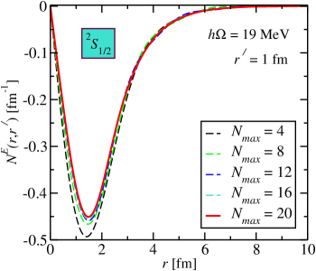
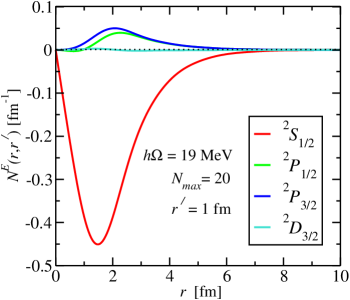
Figure 17: The exchange part of the norm kernel of the n+⁴He system. Left, the convergence with the size of the basis of the ⁴He wave function for the ${}^{2}S_{1/2}$ channel. Right, results for channels are compared. The chiral EFT NN potential was used.

In Fig. 17, we show the exchange part of the norm kernel for the n+⁴He system, in particular the second term of Eq. (78) multiplied by $rr^{\prime}$. It is apparent that we are able to reach convergence for the kernel. Furthemore, the ${}^{2}S_{1/2}$ channel shows, as it should the effect of the Pauli principle. Indeed, the ⁴He wave function is dominated by the four nucleon $s$-shell configuration. The Pauli principle prevents adding the fifth nucleon to the same shell.

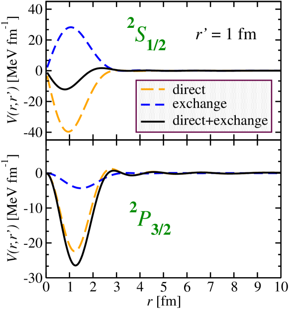
Figure 18: The NN potential direct and exchange terms of the Hamiltonian kernel of the n+⁴He system. The ${}^{2}S_{1/2}$ and ${}^{2}P_{3/2}$ channels are compared. The low-momentum NN potential of Ref. [60] was used in the $14\hbar\Omega$ model space with the HO frequency of $\hbar\Omega=18$ MeV.

In Fig. 18, we show the direct and the exchange contributions of the NN potential to the Hamiltonian kernel as well as their sum for the n+⁴He system. Again, the Pauli principle is manifest in the ${}^{2}S_{1/2}$ channel. We were able to obtain the presented results using wave functions expanded both in the Jacobi-coordinate and the SD basis. The two independent calculations gave identical results as expected. A converged calculation of the ${}^{2}S_{1/2}$ phase shift together with experimental data is presented in Fig. 19. Full details regarding this approach are given in Ref. [61].

Figure 19: The calculated ${}^{2}S_{1/2}$ phase shift for the n+⁴He system compared with experimental data. The low-momentum NN potential of Ref. [60] was used in the $16\hbar\Omega$ model space with the HO frequency of $\hbar\Omega=18$ MeV.

6 Conclusions

The ab initio NCSM evolved into a powerful many-body technique. Presently, it is the only method capable to use interactions derived within the chiral EFT for systems of more than four nucleons, in particular for mid-$p$-shell nuclei. Among its successes is the demonstration of importance of the NNN interaction for nuclear structure. Applications to nuclear reactions with a proper treatment of long-range properties are under development. Extension to heavier nuclei is achieved through the importance-truncated NCSM [62]. Within this approach, ab initio calculations for nuclei as heavy as ⁴⁰Ca become possible.

- [1] \BYL.D. Faddeev \INZh. Eksp. Teor. Fiz. 39 1960 1459 [\INSov. Phys.-JETP 12 1961 1014]
- [2] \BYC.R. Chen, G.L. Payne, J.L. Friar, and B.F. Gibson \INPhys. Rev. C 31 1985 2266
- [3] \BYJ.L. Friar, G.L. Payne, V.G.J. Stoks, and J.J. de Swart \INPhys. Lett. B 311 1993 4
- [4] \BYA. Nogga, D. Hüber, H. Kamada, and W. Glöckle \INPhys. Lett. B 409 1997 19
- [5] \BYO. A. Yakubovsky \INSov. J. Nucl. Phys. 5 1967 937
- [6] \BYW. Glöckle and H. Kamada \INPhys. Rev. Lett. 71 1993 971
- [7] \BYF. Ciesielski and J. Carbonell \INPhys. Rev. C 58 1998 58; \BYF. Ciesielski, J. Carbonell, and C. Gignoux \INNucl. Phys. A 631 1998 653c
- [8] \BYM. Viviani, A. Kievsky, and S. Rosati \INFew-Body Systems 18 1995 25
- [9] \BYN. Barnea, W. Leidemann and G. Orlandini \INNucl. Phys. A 650 1999 427
- [10] \BYB. S. Pudliner, V. R. Pandharipande, J. Carlson, S. C. Pieper and R. B. Wiringa \INPhys. Rev. C 56 1997 1720; \BYR. B. Wiringa, S. C. Pieper, J. Carlson, V. R. Pandharipande \INPhys. Rev. C 62 2000 014001; \BYS. C. Pieper and R. B. Wiringa \INAnn. Rev. Nucl. Part. Sci. 51 2001 53; \BYS. C. Pieper, K. Varga and R. B. Wiringa \INPhys. Rev. C 66 2002 044310
- [11] \BYH. Kamada et al. \INPhys. REv. C 64 2001 044001
- [12] \BYR. F. Bishop, M. F. Flynn, M. C. Boscá, E. Buendía and R. Guardiola \INPhys. Rev. C 42 1990 1341
- [13] \BYJ. H. Heisenberg and B. Mihaila \INPhys. Rev. C 59 1999 1440
- [14] \BYK. Kowalski et al. \INPhys. Rev. Lett. 92 2004 132501
- [15] \BYM. Włoch et al. \INPhys. Rev. Lett. 94 2005 212501
- [16] \BYP. Navrátil, J. P. Vary, and B. R. Barrett \INPhys. Rev. Lett. 84 2000 5728
- [17] \BYL. Trlifaj \INPhys. Rev. C 5 1972 1534
- [18] \BYP. Navrátil, G. P. Kamuntavičius and B. R. Barrett \INPhys. Rev. C 61 2000 044001
- [19] \BYP. Navrátil, B. R. Barrett, and W. Glöckle \INPhys. Rev. C 59 1999 611
- [20] \BYK. Suzuki and S.Y. Lee \INProg. Theor. Phys. 64 1980 2091
- [21] \BYK. Suzuki \INProg. Theor. Phys. 68 1982 246; \BYK. Suzuki and R. Okamoto \INProg. Theor. Phys. 70 1983 439
- [22] \BYK. Suzuki \INProg. Theor. Phys. 68 1982 1999; \BYK. Suzuki and R. Okamoto \INProg. Theor. Phys. 92 1994 1045
- [23] \BYP. Navrátil and W. E. Ormand \INPhys. Rev. C 68 2003 034305
- [24] \BYA. Nogga, P. Navrátil, B. R. Barrett and J. P. Vary \INPhys. Rev. C732006064002
- [25] \BYI. Stetcu, B. R. Barrett, P. Navratil, J. P. Vary \INPhys. Rev. C 71 2005 044325
- [26] \BYD. R. Entem and R. Machleidt \INPhys. Rev. C682003041001(R)
- [27] \BYP. Navrátil and W. E. Ormand \INPhys. Rev. Lett. 88 2002 152502
- [28] \BYP. Navrátil and E. Caurier \INPhys. Rev. C 69 2004 014311
- [29] \BYM. Viviani, L. E. Marcucci, S. Rosati, A. Kievsky and L. Girlanda \INFew-Body Systems 392006159
- [30] \BYE. Caurier, G. Martinez-Pinedo, F. Nowacki, A. Poves, J. Retamosa and A. P. Zuker \INPhys. Rev. C 5919992033; \BYE. Caurier and F. Nowacki \INActa Physica Polonica B 301999705
- [31] \BYS. Weinberg \INPhysica96A1979327; \INPhys. Lett. B2511990228; \INNucl. Phys. B36319913; \BYJ. Gasser et al. \INAnn. of Phys. 1581984142; \INNucl. Phys. B2501985465
- [32] \BYV. Bernard, N. Kaiser, and Ulf-G. Meißner \INInt. J. Mod. Phys. E41995193
- [33] \BYC. Ordonez, L. Ray, and U. van Kolck \INPhys. Rev. Lett.7219941982; \INPhys. Rev. C5319962086
- [34] \BYU. van Kolck \INProg. Part. Nucl. Phys.431999337
- [35] \BYP. F. Bedaque and U. van Kolck \INAnn. Rev. Nucl. Part. Sci.522002339; \BYE. Epelbaum \INProg. Part. Nucl. Phys. 572006654
- [36] \BYU. van Kolck\INPhys. Rev. C4919942932
- [37] \BYE. Epelbaum, A. Nogga, W. Glöckle, H. Kamada, Ulf-G. Meissner and H. Witala \INPhys. Rev. C660640012002
- [38] \BYE. Epelbaum\INPhys. Lett. B2006639
- [39] \BYP. Navrátil, V. G. Gueorguiev, J. P. Vary, W. E. Ormand, and A. Nogga \INPhys. Rev. Lett. 99 2007 042501
- [40] \BYA. C. Hayes, P. Navrátil and J. P. Vary \INPhys. Rev. Lett. 91 2003 012502
- [41] \BYJ. P. Vary “The Many-Fermion-Dynamics Shell-Model Code”, Iowa State University, 1992, unpublished.
- [42] \BYP. Navrátil \INPhys. Rev. C702004054324
- [43] \BYE. Adelberger et al. \INRev. Mod. Phys. 70 1998 1265
- [44] \BYSNO Collaboration, S. N. Ahmed et al. \INPhys. Rev. Lett. 92 2004 181301
- [45] \BYS. Couvidat, S. Turck-Chièze, and A. G. Kosovichev \INAstrophys. J. 599 2003 1434
- [46] \BYJ. N. Bahcall and M. H. Pinsonneault \INPhys. Rev. Lett. 92 2004 121301
- [47] \BYP. Navrátil, C. A. Bertulani and E. Caurier \INPhys. Lett. B6342006191
- [48] \BYP. Navrátil, C. A. Bertulani and E. Caurier \INPhys. Rev. C732006065801
- [49] \BYR. Machleidt\INPhys. Rev. C632001024001
- [50] \BYH. Esbensen and G. F. Bertsch \INNucl. Phys. A 600 1996 37
- [51] \BYR. G. H. Robertson \INPhys. Rev. C 7 1973 543
- [52] \BYA. R. Junghans, E. C. Mohrmann, K. A. Snover, T. D. Steiger, E. G. Adelberger, J. M. Casandjian, H. E. Swanson, L. Buchmann, S. H. Park, A. Zyuzin, and A. M. Laird \INPhys. Rev. C 68 2003 065803
- [53] \BYN. Iwasa et al. \INPhys. Rev. Lett. 83 1999 2910; \BYB. Davids et al. \INPhys. Rev. Lett. 86 2001 2750; \BYF. Schumann et al. \INPhys. Rev. Lett. 90 2003 232501;
- [54] \BYB. T. Kim, T. Izumuto and K. Nagatani \INPhys. Rev. C 23 1981 33
- [55] \BYK. M. Nollett\INPhys. Rev. C 63 2001 054002
- [56] \BYC. R. Brune, R. W. Kavanagh and C. Rolfs Phys. Rev. C 50 1994 2205
- [57] \BYP. Navrátil, C. A. Bertulani and E. Caurier \INNucl. Phys. A7872007539c
- [58] \BYY. C. Tang, M. LeMere and D. R. Thompson \INPhys. Rep. 47 1978 167; \BYK. Langanke and H. Friedrich Advances in Nuclear Physics, chapter 4., Plenum, New York, 1987; \BYR. G. Lovas, R. J. Liotta, A. Insolia, K. Varga and D. S. Delion \INPhys. Rep. 294 1998 265
- [59] \BYP. Navrátil \INPhys. Rev. C 70 2004 014317
- [60] \BYS.K. Bogner, T. T. S. Kuo, and A. Schwenk \INPhys. Rept. 386 2003 1
- [61] \BYS. Quaglioni and P. Navrátil to be published.
- [62] \BYR. Roth and P. Navrátil \INPhys. Rev. Lett 99 2007 092501