Observational constraints on late-time $\Lambda(t)$ cosmology

Abstract

The cosmological constant $\Lambda$, i.e., the energy density stored in the true vacuum state of all existing fields in the Universe, is the simplest and the most natural possibility to describe the current cosmic acceleration. However, despite its observational successes, such a possibility exacerbates the well known $\Lambda$ problem, requiring a natural explanation for its small, but nonzero, value. In this paper we study cosmological consequences of a scenario driven by a varying cosmological term, in which the vacuum energy density decays linearly with the Hubble parameter, $\Lambda\propto H$. We test the viability of this scenario and study a possible way to distinguish it from the current standard cosmological model by using recent observations of type Ia supernova (Supernova Legacy Survey Collaboration), measurements of the baryonic acoustic oscillation from the Sloan Digital Sky Survey and the position of the first peak of the cosmic microwave background angular spectrum from the three-year Wilkinson Microwave Anisotropy Probe.

I Introduction

The nature of the mechanism behind the current cosmic acceleration constitutes a major problem nowadays in Cosmology rev . Even though almost all observational data available so far are in good agreement with the simplest possibility, i.e., a vacuum energy plus cold dark matter ($\Lambda$CDM) scenario, it is becoming rather consensual that in order to better understand the nature of the dark components of matter and energy, one must also consider more complex models as, for instance, scenarios with interaction in the dark sector cq .

In this regard, the simplest examples of interacting dark matter/dark energy models are scenarios with vacuum decay [$\Lambda$(t)CDM]. In reality, $\Lambda$(t)CDM cosmologies constitute the special case in which the ratio of the dark energy pressure to its energy density, $\omega$, is exactly $-1$ Lambda(t) ; lambdat . This kind of model may be based on the idea that dark energy is the manifestation of vacuum quantum fluctuations in the curved space-time, after a renormalization in which the divergent vacuum contribution in the flat space-time is subtracted. The resulting effective vacuum energy density will depend on the space-time curvature, decaying from high initial values to smaller ones as the universe expands 1 . As a result of conservation of total energy, implied by Bianchi identities, the variation of vacuum density leads either to particle production or to an increasing in the mass of dark matter particles, two general features of decaying vacuum or, more generally, of interacting dark energy models jsa .

Naturally, the precise law of vacuum density variation depends on a suitable derivation of the vacuum contribution in the curved background, which is in general a difficult task. In this regard, however, a viable possibility is initially to consider a de Sitter space-time and estimate the renormalized vacuum contribution with help of thermodynamic reasonings as, e.g., those in line with the holographic conjecture Holography . The resulting ansatz is $\Lambda\approx(H+m)^{4}-m^{4}$, where $H$ is the Hubble parameter and $m$ is a cutoff imposed to regularize the vacuum contribution in flat space-time (the next step is to consider a quasi-de Sitter background, with a slowly decreasing $H$. In this case, the above ansatz may be considered a good approximation, but with the vacuum density decaying with time.). In the early-time limit, with $H>>m$, we have $\Lambda\approx H^{4}$. By using this scaling law for the vacuum density and introducing a relativistic matter component, some of us have obtained from the Einstein equations an interesting solution with the following features 2 . Firstly, the Universe undergoes an empty, quasi-de Sitter phase, with $H\approx 1$, which in the asymptotic limit of infinite past tends to de Sitter solution with $H=1$ (in Planck units). However, at a given time, the vacuum undertakes a fast phase transition, with $\Lambda$ decreasing to nearly zero in a few Planck times, producing a considerable amount of radiation. In this sense, this can be understood as a non-singular inflationary scenario, with a semi-eternal quasi-de Sitter phase originating a radiation dominated universe.

The subsequent evolution of vacuum energy essentially depends on the masses of the produced particles. If we apply the energy-time uncertainty relation to the process of matter production, we will conclude that massive particles can be produced only at very early times, when $H$ is very high. Therefore, baryonic particles and massive dark matter (as supersymmetric particles and axions) stopped being produced before the time of electroweak phase transition. On the other hand, the late-time production of photons and massless neutrinos must be forbidden by some selection rule, otherwise the Universe would be completely different from the one observed today. Thus, if no other particle is produced, the vacuum density stops decaying at very early times, and for late times we have a standard universe, with the presence of a genuine cosmological constant (some thermodynamic considerations, in line with the holographic principle, permit to infer the value of this constant, leading to $\Lambda\approx m^{6}$ 1 ; 2 ).

In order to have a decaying vacuum density at the present time, the produced dark particles should have a mass as small as $10^{-65}$g. Here, we have considered the possibility of a late-time decaying $\Lambda$, and compared the consequent cosmological scenario with the constraints imposed by current observations 3 ; 4 . In such a limit, $H<<m$ and $\Lambda\approx m^{3}H$, leading again to $\Lambda\approx m^{6}$ in the de Sitter limit. From a qualitative point of view, we have found no important difference between this $\Lambda(t)$ scenario and the flat $\Lambda$CDM model 3 . After the phase transition described above the Universe enters a radiation-dominated phase, followed by a matter-dominated era long enough for structure formation, which tends asymptotically to a de Sitter universe with vacuum dominating again. The only important novelty, related to matter production, is a late-time suppression of the density contrast of matter, which may constitute a potential solution to the cosmic coincidence problem 5 . Moreover, the analysis of the redshift-distance relation for supernovae of type Ia, particularly with the Supernova Legacy Survey (SNLS) data set, has shown a good fit, with present values of $H$ and the relative density of matter in accordance with other observations 4 .

In this paper, we go a little further in our investigation and study new observational consequences of the $\Lambda$(t)CDM scenario described above. We use to this end distance measurements from type Ia supernovae (SNe Ia), measurements of the baryonic acoustic oscillations (BAO) and the position of the first peak of the cosmic microwave background (CMB). We show that, besides the interesting cosmic history of this class of $\Lambda$(t)CDM models, a conventional, spatially flat $\Lambda$CDM model is only slightly favored over them by the current observational data.

II The model

In a spatially flat FLRW space-time the Friedmann and the conservation equations can be written, respectively, as

$$\rho_{T}=3H^{2}\;,$$ (1)

and

$$\dot{\rho}_{T}+3H(\rho_{T}+p_{T})=0\;,$$ (2)

where $\rho_{T}$ and $p_{T}$ are the total energy density and pressure, respectively. If we consider that the cosmic fluid is composed of matter with energy density $\rho_{m}$ and pressure $p_{m}$, and of a time-dependent vacuum term with energy density $\rho_{\Lambda}=\Lambda$ and pressure $p_{\Lambda}=-\Lambda$, we obtain

$$\dot{\rho}_{m}+3H(\rho_{m}+p_{m})=-\dot{\Lambda}\;,$$ (3)

which shows that matter is not independently conserved, with the decaying vacuum playing the role of a matter source. Throughout our analysis we assume that baryons are independently conserved at late times, being not produced at the expenses of the decaying vacuum. This amounts to saying that we will postulate, in addition to Eq. (3), a conservation equation for baryons, i.e., $\dot{\rho}_{b}+3H(\rho_{b}+p_{b})=0$, where $\rho_{b}$ and $p_{b}$ refer to baryon density and pressure.

From the above equations and considering our late-time ansatz $\Lambda=\sigma H$ ($\sigma$ is a positive constant of the order of $m^{3}$), the evolution equation reads

$$2\dot{H}+3H^{2}-\sigma H=0\;.$$ (4)

Now, with the conditions $H>0$ and $\rho_{m}>0$, the integration of the above equation leads to the following expression for the scale factor,

$$a(t)=C\left[\exp\left(\sigma t/2\right)-1\right]^{\frac{2}{3}}\;,$$ (5)

where $C$ is the first integration constant and the second one was chosen so that $a=0$ at $t=0$. From these equations, it is straightforward to show that at early times the above expression reduces to the Einstein-de Sitter solution whereas at late times it tends to the de Sitter universe.

As stated earlier, $\Lambda=\sigma H$ and, therefore, $\rho_{m}=3H^{2}-\sigma H$. By using solution (5), one can also show that

$$\rho_{m}=\frac{\sigma^{2}C^{3}}{3a^{3}}+\frac{\sigma^{2}C^{3/2}}{3a^{3/2}}\;,$$ (6)

and

$$\Lambda=\frac{\sigma^{2}}{3}+\frac{\sigma^{2}C^{3/2}}{3a^{3/2}}.$$ (7)

The above expressions can be easily understood as follows. The first terms in the r.h.s. are the expected scaling laws for matter density and the cosmological constant in the case of a non-decaying vacuum while the second ones are related to the time variation of the vacuum density and the concomitant matter production. As expected, at early times matter dominates, with its density scaling with $a^{-3}$, and the matter production process is negligible. On the other hand, at late times the vacuum term dominates, as should be in a de Sitter universe.

From Eqs. (1), (6) and (7), the evolution of the Hubble parameter as a function of the redshift can be written as

$$H(z)=H_{0}\left[1-\Omega_{m}+\Omega_{m}(1+z)^{3/2}\right],$$ (8)

where $H_{0}$ and $\Omega_{m}$ are, respectively, the present values of the Hubble parameter and of the relative energy density of matter. Note that, due to the matter production, this expression is rather different from that found in the context of the standard $\Lambda$CDM case. In particular, if $\Lambda=0$ and $\Omega_{m}=1$, we obtain $H(z)=H_{0}(1+z)^{3/2}$, leading to $\rho_{m}=3H_{0}^{2}(1+z)^{3}$, as expected for the Einstein-de Sitter scenario.

III Observational constraints

Extending and updating previous results 4 , we study in this Section some observational consequences of the class of $\Lambda$(t)CDM scenarios discussed above. Note that, similarly to the standard $\Lambda$CDM case, this class of models has only two independent parameters, $H_{0}$ and $\Omega_{m}$ [see Eq. (8)]. The best-fit values for these quantities will be determined on the basis of a statistical analysis of recent type Ia supernovae (SNe Ia) measurements, as given by the SNLS Collaboration Legacy , the distance to the baryonic acoustic oscillations (BAO) from the Sloan Digital Sky Survey (SDSS) Eisenstein , and the position of the first peak in the spectrum of anisotropies of CMB radiation from the three-year Wilkinson Microwave Anisotropy Probe (WMAP) WMAP (for more details on the statistical analysis discussed below we refer the reader to Ref. refs ).

III.1 SNe Ia observations

The predicted distance modulus for a supernova at redshift $z$, given a set of parameters $\mathbf{s}$, is

$$\mu_{p}(z|\mathbf{s})=m-M=5\,\mbox{log}d_{L}+25,$$ (9)

where $m$ and $M$ are, respectively, the apparent and absolute magnitudes, the complete set of parameters is $\mathbf{s}\equiv(H_{0},\Omega_{m})$, and $d_{L}$ stands for the luminosity distance (in units of megaparsecs),

$$d_{L}=c(1+z)\int_{x^{\prime}}^{1}{dx\over x^{2}{H}(x;\mathbf{s})},$$ (10)

with $x^{\prime}={a(t)\over a_{0}}=(1+z)^{-1}$ being a convenient integration variable, and ${H}(x;\mathbf{s})$ the expression given by Eq. (8).

We estimated the best fit to the set of parameters $\mathbf{s}$ by using a $\chi^{2}$ statistics, with

$$\chi^{2}=\sum_{i=1}^{N}{\frac{\left[\mu_{p}^{i}(z|\mathbf{s})-\mu_{o}^{i}(z)\right]^{2}}{\sigma_{i}^{2}}},$$ (11)

where $\mu_{p}^{i}(z|\mathbf{s})$ is given by Eq. (9), $\mu_{o}^{i}(z)$ is the extinction corrected distance modulus for a given SNe Ia at $z_{i}$, and $\sigma^{2}_{i}=\sigma^{2}_{(\mu_{B})}+\sigma^{2}_{int}$, where $\sigma^{2}_{(\mu_{B})}$ is the variance in the individual observations and $\sigma^{2}_{int}$ stands for the intrinsic dispersion for each SNe Ia absolute magnitude. Since we use in our analysis the SNLS collaboration sample Legacy , $N=115$. As discussed in Ref. 4 , the best-fit values for this analysis is obtained for $h=0.70$ and $\Omega_{m}=0.33$, with reduced $\chi^{2}_{r}=1.01$. At $95\%$ of confidence level, we also find $0.69<h<0.71$ and $0.28<\Omega_{m}<0.37$. The $2$-dimensional contours shown in the Figures are obtained from the traditional frequentist confidence intervals (based on the $\Delta\chi^{2}$ approach and assuming that errors are normally distributed).

III.2 Baryonic acoustic oscillations

     

Figure 1: Left) Superposition of the confidence regions in the $\Omega_{\rm{m}}-h$ plane for our analysis of SNe Ia, BAO and CMB. Right) The same for a spatially flat $\Lambda$CDM model.

The use of BAO to test dark energy models is usually made by means of the parameter ${\cal{A}}$, i.e., Eisenstein

$${\cal{A}}=D_{V}\frac{\sqrt{\Omega_{m}H_{0}^{2}}}{zc}\;,$$ (12)

where $z=0.35$ is the typical redshift of the sample and $D_{V}$ is the dilation scale, defined as

$$D_{V}(z)=\left[D_{M}(z)^{2}\frac{zc}{H(z)}\right]^{1/3}\;,$$ (13)

with the comoving distance $D_{M}$ given by

$$D_{M}(z)=c\int_{0}^{z}\frac{dz^{\prime}}{H(z^{\prime})}\;.$$ (14)

An important aspect worth emphasizing at this point is that the value of ${\cal{A}}$ is obtained from the data in the context of a $\Lambda$CDM model, and can be considered a good approximation only for some class of dark energy models EarlyDE . In particular, two conditions are implicitly assumed to be valid Eisenstein . First, the evolution of matter density perturbations during the matter-dominated era must be similar to the $\Lambda$CDM case, at least until the characteristic redshift $z=0.35$. Second, the comoving distance to the horizon at the time of equilibrium between matter and radiation must scale with $(\Omega_{m}H_{0}^{2})^{-1}$. However, none of the above conditions are satisfied in the present model because of the matter production associated to the vacuum decay. As will be shown in a forthcoming publication 5 , if matter is homogeneously produced there is a suppression in its density contrast for $z<5$, that is, after the period of galaxy formation (this will eventually imply a higher value of $\Omega_{m}$ in order to fit the observed mass power spectrum).

On the other hand, as radiation is independently conserved, its relative energy density for $z>>1$ is given by $\Omega_{r}z^{4}$, where $\Omega_{r}$ is its present value. With the help of (8) we can see that, in the same limit $z>>1$, the relative density of matter is $\Omega_{m}^{2}z^{3}$ (with the extra factor $\Omega_{m}$ being due to the matter production between $t(z)$ and the present time). By equating the two densities, we obtain the redshift of equilibrium between matter and radiation, given by $z_{rm}=\Omega_{m}^{2}/\Omega_{r}$. Therefore, after including conserved radiation into (8) (see equation (17) below) and taking $z>>1$, we have $r_{H}(z_{rm})\approx c\sqrt{\rho_{r}/6}(\Omega_{m}H_{0})^{-2}$, where $\rho_{r}$ is the present value of the radiation density (while in the $\Lambda$CDM case we would obtain $r_{H}(z_{rm})\approx c\sqrt{\rho_{r}/6}(\Omega_{m}H_{0}^{2})^{-1}$, as stated above). Thus, one can see that the parameter ${\cal{A}}$ is not appropriate to test the model, and we will use instead the dilation scale $D_{V}$, which is weakly sensitive to the cosmological evolution before $z=0.35$. By combining our function $H(z)$, given by (8), into (13)-(14) we can find the region in the $\Omega_{m}-H_{0}$ plane which gives the observed value $D_{V}=(1370\pm 64)$ Mpc ($1\sigma$) Eisenstein . The BAO bands in the $\Omega_{m}-H_{0}$ parametric space are shown in Fig. 1.

III.3 The first peak of CMB

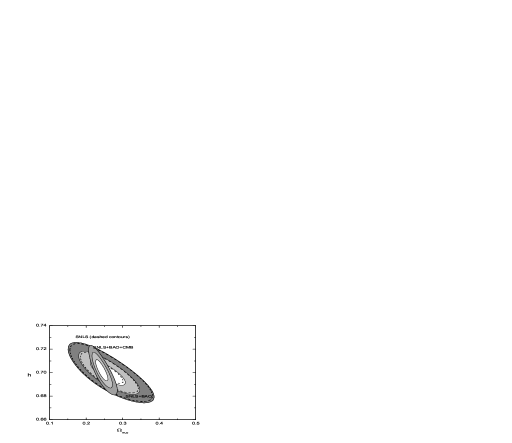
Figure 2: Left) Confidence regions (68.3%, 95.4% and 99.7%) in the $\Omega_{\rm{m}}-h$ plane for a joint analysis involving SNe Ia, BAO and CMB data. As indicated, the dashed lines stand for the SNe Ia results of Ref. 4 . In both panels, the largest contours represent the joint analysis of SNe Ia plus BAO measurements whereas the smallest ones arises when the CMB data are included in the analysis. Right) The same for a spatially flat $\Lambda$CDM model.

The two tests we have previously described depend on the physics at low and intermediate redshifts (until $z\sim 1$) and will lead, as we will see, to very similar results. As a complementary test, involving high-$z$ measurements, let us consider the position of the first peak in the spectrum of CMB anisotropies. Since in the present model there is no production of baryonic matter or radiation and the spatial curvature is null, we expect that a correct position of the first peak is enough to guarantee a spectral profile similar to the $\Lambda$CDM one, provided the spectrum of primordial fluctuations is the same.

In the context of a large class of dark energy models this test is performed by comparing the predicted shift parameter with the $\Lambda$CDM value. However, this is only valid if the acoustic horizon at the time of last scattering is the same Raul . This is not true in the present model because, as we have already shown, for the same values of $H_{0}$ and $\Omega_{m}$ we have different expressions for cosmological parameters at high redshifts, due to the process of matter production. Therefore, in order to perform a correct test, we have to explicitly calculate the acoustic scale in the model and then compare with the measured position of the peak.

The acoustic scale, defined as the ratio between the comoving distance to the surface of last scattering and the radius of the acoustic horizon at that time, is then given by

$$l_{A}=\frac{\pi\int_{0}^{z_{ls}}\frac{dz}{H(z)}}{\int_{z_{ls}}^{\infty}\frac{c_{s}}{c}\frac{dz}{H(z)}},$$ (15)

where $z_{ls}$ is the redshift of last scattering, and

$$c_{s}=c\left(3+\frac{9}{4}\frac{\Omega_{b}}{\Omega_{\gamma}z}\right)^{-1/2}$$ (16)

is the sound velocity. Here, $\Omega_{b}$ and $\Omega_{\gamma}$ are, respectively, the present relative energy densities of baryons and photons.

The function $H(z)$ to be used in Eq. (15) must now include radiation. As this component is independently conserved, scaling with $a^{-4}$, the appropriate generalization of Eq. (8) is given by

$$\frac{H(z)}{H_{0}}\approx\left\{\left[1-\Omega_{m}+\Omega_{m}(1+z)^{3/2}\right]^{2}+\Omega_{r}(1+z)^{4}\right\}^{1/2}.$$ (17)

Therefore, apart from our two free parameters $H_{0}$ and $\Omega_{m}$, in order to determine the acoustic scale we need the present values of the energy densities of radiation, photons and baryons, as well as an expression for $z_{ls}$. Since radiation and baryons are independently conserved, and we want to preserve the spectrum profile as well as the nucleosynthesis constraints, we will take for these densities the same values obtained from CMB observations in the context of the $\Lambda$CDM model CMB : $\Omega_{\gamma}h^{2}\approx 2.45\times 10^{-5}$, $\Omega_{r}h^{2}\approx 4.1\times 10^{-5}$ and $\Omega_{b}h^{2}\approx 0.02$.

Concerning $z_{ls}$, its value is not in principle the same as in the $\Lambda$CDM case. To determine its value for a given pair ($\Omega_{m}$,$H_{0}$) we will proceed as follows. First, we obtain the redshift of last scattering $z^{*}_{ls}$ in the $\Lambda$CDM model by means of the current fitting formula Raul , and then we impose that the optical depth has to be the same in both models, that is,

$$\int_{0}^{z_{ls}}\frac{\Gamma(z)}{H(z)}\frac{dz}{1+z}=\int_{0}^{z^{*}_{ls}}\frac{\Gamma(z)}{H^{*}(z)}\frac{dz}{1+z},$$ (18)

where $\Gamma$ is the rate of photon scattering and $H^{*}$ is the Hubble parameter in the $\Lambda$CDM context. For the current intervals of $H_{0}$ and $\Omega_{m}$, the relative differences between $z_{ls}$ and $z^{*}_{ls}$ are typically as small as $1\%$.

For a scale invariant $\Lambda$CDM model with spectral index $n=1$, the position of the first peak after including the effect of plasma driving is given by the fitting expression Tegmark

$$l_{1}=l_{A}(1-\delta_{1}),$$ (19)

where

$$\delta_{1}=0.267\left(\frac{r}{0.3}\right)^{0.1},$$ (20)

with $r\equiv\rho_{\gamma}(z_{ls})/\rho_{m}(z_{ls})$. Since the plasma driving depends essentially on pre-recombination physics, we will therefore assume that the above fitting formulae are a good approximation to the present $\Lambda(t)$ model. In our case, the parameter $r$ is given by

$$r=\frac{\Omega_{\gamma}}{\Omega_{m}^{2}}z_{ls}.$$ (21)

Finally, from the above results we can determine the region of the $\Omega_{m}$-$H_{0}$ plane for which the first peak has the position currently observed by WMAP, i.e., $l_{1}=220.8\pm 0.7$ ($1\sigma$) WMAP . As in the case of BAO, the CMB bands in the $\Omega_{m}-H_{0}$ parametric space is shown in Fig. 1.

III.4 Results and discussions

The superposition of the confidence regions and bands corresponding to our analysis of SNe Ia, BAO and CMB observations is shown in Figure 1. For the sake of comparison, the right panel shows the same analysis for the standard $\Lambda$CDM model. From these analysis, we note that, although not very restrictive and parallel to the SNe Ia contours, the BAO bands can be statistically combined with SNe Ia data providing constraints on the $\Omega_{m}-H_{0}$ plane. At $2\sigma$ level, we find $h=0.70\pm 0.01$ and $\Omega_{m}=0.32\pm 0.05$, with reduced $\chi^{2}_{r}\simeq 1.00$. The inclusion of CMB data into our analysis in turn makes the complete joint analysis more restrictive but also shows that the concordance is as good as in the standard $\Lambda$CDM case, and that the $\Lambda$(t)CDM model discussed here cannot be ruled out. It can be anticipated from Figure 1 that the data will prefer higher values of the matter density parameter, while the Hubble parameter is expected to be slightly smaller than the current accepted values. In order to confirm this qualitative discussion, Figure 2 shows the results of our joint statistical analysis (SNe Ia + BAO + CMB). At $2\sigma$ level, we find $h=0.69\pm 0.01$ and $\Omega_{m}=0.36\pm 0.01$, with reduced $\chi^{2}_{r}=1.01$. For the sake of comparison, the same analysis for the $\Lambda$CDM case is also shown in the right panel of Fig. 2.

Finally, with the above best-fit values for the parameters, we can calculate the total expanding age for this class of $\Lambda$(t)CDM models, given by 3 ; 4

$$t_{0}=H_{0}^{-1}\frac{\frac{2}{3}\ln(\Omega_{\rm{m}})}{\Omega_{\rm{m}}-1}\simeq 15.0\hskip 0.85355pt\mbox{Gyr}\;,$$ (22)

as well as the redshift of transition from a decelerated expansion to the current accelerating phase, i.e., $z_{T}\approx 1.3$. Note that both values are slightly higher than, but of the same order of, the standard ones.

IV Final remarks

By using the most recent cosmological observations, we have discussed the observational viability of a class of $\Lambda$(t)CDM scenarios in which $\Lambda\propto H$, as well as a possible way to distinguish it from the standard $\Lambda$CDM model in what concerns the general characteristics of the predicted cosmic evolution. As discussed earlier, these $\Lambda$(t)CDM models have some interesting features as, e.g., the association of dark energy with vacuum fluctuations, the circumvention of the cosmological constant problem by subtracting the flat space-time contribution from the curved space-time vacuum density, and the possible (but not necessary) link between dark matter and massive gravitons.

We have presented some quantitative results which clearly show that, even in the current stage of the Universe evolution, our decaying vacuum scenario is very similar to the standard one. We have statistically tested the viability of the model by using recent SNe Ia observations and measurements of the BAO and the first peak of the CMB spectrum. At 95.4% c.l., a joint analysis involving SNe Ia + BAO provides the intervals $0.69\leq h\leq 0.71$ and $0.28\leq\Omega_{m}\leq 0.37$, which are in good agreement with the values of the Hubble and the matter density parameters obtained from independent analysis hst ; omega . When the position of the first peak of CMB anisotropies is included in the analysis, the best-fit value for the relative matter density is increased, $\Omega_{m}\simeq 0.36$. This result cannot rule out the model, and it may be indicating that, besides the interesting cosmic history of this class of $\Lambda$(t)CDM models, a conventional, spatially flat $\Lambda$CDM model is only slightly favored over them by the current observational data. Still on the best-fit for $\Omega_{m}$, we note that such a higher matter density is something to be more investigated by means of other cosmological or dynamical tests as, e.g., the predicted mass power spectrum in the context of the model. As we have discussed earlier, a higher matter density is necessary to compensate the late-time suppression of the density contrast owing to matter production 5 . Another possibility will be provided by future supernovae observations, since the present model starts to diverge from the standard one for higher redshifts 4 .

Finally, we should also emphasize two aspects to be considered before a definite conclusion about the comparison between the present model and the flat standard scenario. First, that in our study of CMB we have used parameter values and fitting formulae that are strictly correct for the $\Lambda$CDM case, particularly the expression giving the position of the first peak for a given acoustic scale [equation (19)]. In spite of our reasons to consider that use as a good approximation, it can lead to bias in our results. If that is the case, only a more complete analysis of CMB would rule out or corroborate the model. The second aspect is of theoretical character. As discussed in the Introduction, our ansatz for the variation of $\Lambda$, if genuine, is a good approximation only for quasi-de Sitter backgrounds. Naturally, our Universe, although dominated by a cosmological term, is far away from the asymptotic de Sitter state, with matter still giving an important contribution to the cosmic fluid. Only a more profound theoretical study, on the basis of quantum field theories in the expanding background, could establish the degree of applicability and limits of that approximation.

References

- (1) V. Sahni and A. A. Starobinsky, Int. J. Mod. Phys. D9, 373 (2000); P. J. E. Peebles and B. Ratra Rev. Mod. Phys. 75, 559 (2003); T. Padmanabhan, Phys. Rept. 380, 235 (2003); E. J. Copeland, M. Sami and S. Tsujikawa, Int. J. Mod. Phys. D15, 1753 (2006); J. S. Alcaniz, Braz. J. Phys. 36, 1109 (2006).
- (2) L. Amendola, Phys. Rev. D 62, 043511 (2000); J. M. F. Maia and J. A. S. Lima, Phys. Rev. D 65, 083513 (2002); T. Koivisto, Phys. Rev. D 72, 043516 (2005); S. Lee, G. C. Liu and K. W. Ng, Phys. Rev. D 73, 083516 (2006); M. C. Bento, O. Bertolami and N. M. C. Santos, arXiv:gr-qc/0111047; O. Bertolami, F. Gil Pedro and M. Le Delliou, Phys. Lett. B 654, 165 (2007); F. E. M. Costa, J. S. Alcaniz and J. M. F. Maia, arXiv:0708.3800 [astro-ph].
- (3) M. zer and M. O. Taha, Phys. Lett. B171, 363 (1986); Nucl. Phys. B287, 776 (1987); O. Bertolami, Nuovo Cimento Soc. Ital. Fis. B93, 36 (1986).
- (4) K. Freese et al, Nucl. Phys. B287, 797 (1987); W. Chen and Y-S. Wu, Phys. Rev. D41, 695 (1990); M. S. Berman, Phys. Rev. 43, 1075 (1991); D. Pavón, Phys. Rev. D43, 375 (1991); J. C. Carvalho, J. A. S. Lima and I. Waga, Phys. Rev. D46 2404 (1992); A. I. Arbab and A. M. M. Abdel-Rahman, Phys. Rev. D50, 7725 (1994); J. A. S. Lima and J. M. F. Maia, Phys. Rev D49, 5597 (1994); J. A. S. Lima and M. Trodden, Phys. Rev. D53, 4280 (1996); J. M. Overduin and F. I. Cooperstock, Phys. Rev. D58, 043506 (1998); J. M. Overduin, Astrophys. J. 517, L1 (1999); J. Shapiro and J. Sola, Phys. Lett B475, 236 (1999); M. V. John and K.B. Joseph, Phys. Rev. D61, 087304 (2000); O. Bertolami and P. J. Martins, Phys. Rev. D61, 064007 (2000); R. G. Vishwakarma, Gen. Rel. Grav. 33, 1973 (2001); A. S. Al-Rawaf, Mod. Phys. Lett. A14, 633 (2001); R. Schützhold, Phys. Rev. Lett. 89, 081302 (2002); Int. J. Mod. Phys. A17, 4359 (2002); M. K. Mak, J. A. Belinchon, and T. Harko, IJMP D11, 1265 (2002); I. L. Shapiro and J. Sola, JHEP 0202, 006 (2002); W. Zimdahl and D. Pavón, Gen. Rel. Grav. 35, 413 (2003); M. R. Mbonye, IJMP A18, 811 (2003); J. S. Alcaniz and J. M. F. Maia, Phys. Rev. D67, 043502 (2003); I. L. Shapiro, J. Sola, C. Espana-Bonet, and P. Ruiz-Lapuente, Phys. Lett. B574, 149 (2003); J. V. Cunha and R. C. Santos, IJMP D13, 1321 (2004); R. Opher and A. Pellison, Phys. Rev. D70, 063529 (2004); R. Horvat, Phys. Rev. D70, 087301 (2004); C. Espana-Bonet et al. JCAP 0402, 006 (2004); P. Wang and X. Meng, Class. Quant. Grav. 22, 283 (2005); S. Carneiro and J. A. S. Lima, IJMP A20 2465 (2005); S. Carneiro, IJMP D14, 2201 (2005); I. L. Shapiro, J. Sola, and H. Stefancic, JCAP 0501, 012 (2005); E. Elizalde, S. Nojiri, S. D. Odintsov, and P. Wang, Phys. Rev. D71, 103504 (2005); R. Aldrovandi, J. P. Beltrán Almeida, and J. G. Pereira, Grav. & Cosmol. 11, 277 (2005); F. Bauer, Class. Quant. Grav. 22, 3533 (2005); B. Wang, Y. Gong, and E. Abdalla, Phys. Lett. B624, 141 (2005); J. Sola and H. Stefancic, Mod. Phys. Lett. A21, 479 (2006); J. D. Barrow and T. Clifton, Phys. Rev. D73, 103520 (2006); B. Wang, C. Y. Lin, and E. Abdalla, Phys. Lett. B637, 357 (2006); A. E. Montenegro Jr. and S. Carneiro, Class. Quant. Grav. 24, 313 (2007).
- (5) S. Carneiro. Int. J. Mod. Phys. D12, 1669 (2003).
- (6) J. S. Alcaniz and J. A. S. Lima, Phys. Rev. D72, 063516 (2005).
- (7) R. Bousso, Rev. Mod. Phys. 74, 825 (2002); T. Padmanabhan, Phys. Rept. 406, 49 (2005).
- (8) S. Carneiro, Int. J. Mod. Phys. D15, 2241 (2006); J. Phys. A40, 6841 (2007).
- (9) See, for example, M. Novello and R. P. Neves, Class. Quant. Grav. 20, L67 (2003).
- (10) H. A. Borges and S. Carneiro, Gen. Rel. Grav. 37, 1385 (2005).
- (11) S. Carneiro, C. Pigozzo, H. A. Borges and J. S. Alcaniz, Phys. Rev. D74, 23532 (2006) [arXiv:astro-ph/0605607].
- (12) H. A. Borges, S. Carneiro, J. C. Fabris and C. Pigozzo, arXiv:0711.2689 [astro-ph], to appear in Phys. Rev. D.
- (13) P. Astier et al., Astron. Astrophys. 447, 31 (2006).
- (14) D. J. Eisenstein et al., Astrophys. J. 633, 560 (2005).
- (15) G. Hinshaw et al., Astrophys. J. Suppl. 170, 288 (2007); D. N. Spergel et al., Astrophys. J. Suppl. 170, 377 (2007).
- (16) T. Padmanabhan and T. R. Choudhury, Mon. Not. R. Astron. Soc. 344, 823 (2003); P. T. Silva and O. Bertolami, Astrophys. J. 599, 829 (2003); Z.-H. Zhu and M.-K. Fujimoto, Astrophys. J. 585, 52 (2003); J. S. Alcaniz, Phys. Rev. D 65, 123514 (2002) [arXiv:astro-ph/0202492]; S. Nesseris and L. Perivolaropoulos, Phys. Rev. D 70, 043531 (2004); J. S. Alcaniz and N. Pires, Phys. Rev. D 70, 047303 (2004) [arXiv:astro-ph/0404146]; J. S. Alcaniz, Phys. Rev. D 69, 083521 (2004) [arXiv:astro-ph/0312424]; T. R. Choudhury and T. Padmanabhan, Astron. Astrophys. 429, 807 (2005); J. S. Alcaniz and Z.-H. Zhu, Phys. Rev. D 71, 083513 (2005) [arXiv:astro-ph/0411604]; D. Rapetti, S. W. Allen, and J. Weller, Mon. Not. R. Astron. Soc. 360, 555 (2005); Z. K. Guo, Z. H. Zhu, J. S. Alcaniz and Y. Z. Zhang, Astrophys. J. 646, 1 (2006) [arXiv:astro-ph/0603632]; L. Samushia and B. Ratra, Astrophys. J. 650, L5 (2006); M. A. Dantas, J. S. Alcaniz, D. Jain and A. Dev, Astron. Astrophys. 467, 421 (2007) [arXiv:astro-ph/0607060].
- (17) See, for instance, M. Doran, S. Stern and E. Thommes, JCAP 0704, 015 (2007).
- (18) O. Elgaroy and T. Multamaki, astro-ph/0702343.
- (19) P. de Bernardis et al., Nature (London) 404, 955 (2000); S. Hanany et al., Astrophys. J. Lett. 545, L5 (2000); S. Padin et al., ibid, 549, L1 (2001); D. N. Spergel et al., Astrophys. J. Suppl. 148, 175 (2003).
- (20) W. Hu et al., Astrophys. J. 549, 669 (2001).
- (21) W. L. Freedman et al., Astrophys. J. 553, 47 (2001).
- (22) H. A. Feldman, R. Juszkiewicz, P. Ferreira et al., Astrophys. J. 596, L131 (2003).