Parallel multiscale modeling of biopolymer dynamics with hydrodynamic correlations

Abstract

We employ a multiscale approach to model the translocation of biopolymers through nanometer size pores. Our computational scheme combines microscopic Molecular Dynamics (MD) with a mesoscopic Lattice Boltzmann (LB) method for the solvent dynamics, explicitly taking into account the interactions of the molecule with the surrounding fluid. We describe an efficient parallel implementation of the method which exhibits excellent scalability on the Blue Gene platform. We investigate both dynamical and statistical aspects of the translocation process by simulating polymers of various initial configurations and lengths. For a representative molecule size, we explore the effects of important parameters that enter in the simulation, paying particular attention to the strength of the molecule-solvent coupling and of the external electric field which drives the translocation process. Finally, we explore the connection between the generic polymers modeled in the simulation and DNA, for which interesting recent experimental results are available.

I Introduction

Biological systems exhibit a complexity and diversity much richer than the simple solid or fluid systems traditionally studied in physics or chemistry. The powerful quantitative methods developed in the latter two disciplines to analyze the behavior of prototypical simple systems are often difficult to extend to the domain of biological systems. Advances in computer technology and breakthroughs in simulational methods have been constantly reducing the gap between quantitative models and actual biological behavior. The main challenge remains the wide and disparate range of spatio-temporal scales involved in the dynamical evolution of complex biological systems. In response to this challenge, various strategies have been developed recently, which are in general referred to as “multiscale modeling”. These methods are based on composite computational schemes in which information is exchanged between the scales, in either a sequential or a concurrent manner MMS_review .

We have recently developed a multiscale framework which is well suited to address a class of biologically related problems. This method involves different levels of the statistical description of matter (continuum and particle) and is able to handle different scales through the spatial and temporal coupling of a mesoscopic fluid solvent, based on the lattice Boltzmann method LBEa ; LBEb ; LBEc (LB), to a coarse-grained particle level, which employs explicit molecular dynamics (MD). The solvent dynamics does not require any form of statistical ensemble averaging as it is represented through a discrete set of pre-averaged probability distribution functions, which are propagated along straight particle trajectories. This dual field/particle nature greatly facilitates the coupling between the mesoscopic fluid and the atomistic level, which proceeds seamlessy in time and only requires standard interpolation/extrapolation methods for information-transfer in physical space. Full details on this scheme are reported in Ref. ourLBM . LB and MD with Langevin dynamics have been coupled before DUN , but our implementation involves such coupling for long molecules of biological interest. In addition, we have recently developed a parallel version of the code and successfully ported it to the IBM-BlueGene architecture.

Motivated by recent experimental studies, we apply this multiscale approach to the translocation of a biopolymer through a narrow pore. This type of biophysical process is important in phenomena like viral infection by phages, inter-bacterial DNA transduction or gene therapy TRANSL . In addition, it is hoped that this type of process will open a way for ultrafast DNA-sequencing by sensing the base-sensitive electronic signal as the biopolymer passes through a nanopore with attached electrodes. Experimentally, translocation is observed in vitro by pulling DNA molecules through micro-fabricated solid state or membrane channels under the effect of a localized electric field EXPRM . From a theoretical point of view, simplified schemes statisTrans and non-hydrodynamic coarse-grained or microscopic models DynamPRL ; Nelson are able to analyze universal features of the translocation process. This, though, is a complex phenomenon involving the competition between many-body interactions at the atomic or molecular scale, fluid-atom hydrodynamic coupling, as well as the interaction of the biopolymer with wall molecules in the region of the pore. A quantitative description of this complex phenomenon calls for state-of-the art modeling, towards which the results presented here are directed.

II Coupling between Lattice Boltzmann and Molecular Dynamics

In this section we outline the simulation method used to couple the Lattice Boltzmann description for the solvent to the Molecular Dynamics description of the solute. In the LB method the basic quantity is $f_{i}(\vec{x},t)$, representing the probability of finding a “fluid particle” at the spatial mesh location $\vec{x}$ and at time $t$ with discrete speed $\vec{c}_{i}$. We emphasize that the “fluid particles” do not correspond to individual physical particles such as water molecules; they are simply an effective medium for representing the collective motion of such physical particles. Once the discrete distributions $f_{i}$ are known, the local density, flow speed and momentum-flux tensor of the fluid are obtained by a direct summation upon all discrete distributions:

$$\rho(\vec{x},t)=\sum_{i}f_{i}(\vec{x},t)$$ (1)

$$\rho\vec{u}(\vec{x},t)=\sum_{i}f_{i}(\vec{x},t)\vec{c}_{i}$$ (2)

$$\vbox{\halign{#\cr$\leftrightarrow$\crcr\kern-1.0pt\nointerlineskip\cr$\hfil\displaystyle{P}\hfil$\crcr}}(\vec{x},t)=\sum_{i}f_{i}(\vec{x},t)\vec{c}_{i}\vec{c}_{i}$$ (3)

where, for the present study, the standard three-dimensional 19-speed lattice is used LBEc . The fluid populations are advanced in time through the following evolution equation:

$$f_{i}(\vec{x}+\vec{c}_{i}\Delta t,t+\Delta t)=f_{i}(\vec{x},t)+\omega\Delta t(f_{i}-f_{i}^{eq})(\vec{x},t)+F_{i}\Delta t+S_{i}\Delta t$$ (4)

The discrete velocities $\vec{c}_{i}$ connect mesh points to first and second topological neighbors, therefore the fluid particles can only move along the links of a regular lattice and the synchronous particle displacements $\Delta\vec{x}_{i}=\vec{c}_{i}\Delta t$ never take the fluid particles away from the lattice. The right hand side of Eq. (4) represents the effect of fluid-fluid molecular collisions, through a relaxation towards a local equilibrium, $f_{i}^{eq}$, typically a second-order expansion in the fluid velocity of a local Maxwellian with speed $\vec{u}$:

$$f_{i}^{eq}=w_{i}[\beta\vec{u}\cdot\vec{c}_{i}+\frac{\beta^{2}}{2}(\vec{u}\vec{u}\cdot(\vec{c}_{i}\vec{c}_{i}-\frac{1}{\beta}\vbox{\halign{#\cr$\leftrightarrow$\crcr\kern-1.0pt\nointerlineskip\cr$\hfil\displaystyle{I}\hfil$\crcr}})]$$ (5)

where $\beta=1/k_{B}T$ is the inverse temperature, $w_{i}$ a set of weights normalized to unity, and $\leftrightarrow$ $\hfil\displaystyle{I}\hfil$ is the unit tensor in cartesian space. The relaxation frequency $\omega$ controls the kinematic viscosity of the pure fluid:

$$\nu=k_{B}T\left(\frac{1}{\omega}-\frac{\Delta t}{2}\right)$$

The $F_{i}$ term is a stochastic force needed to inject fluctuations in the fluid at the level of fluctuating hydrodynamics, which is local in space and time, and is given by

$$F_{i}=w_{i}\{\sum_{a,b}F^{(2)}_{ab}(c_{ia}c_{ib}-k_{B}T\delta_{ab})+\sum_{a,b,c}F^{(3)}_{abc}g_{iabc}\}$$ (6)

where $F^{(2)}$ is a fluctuating stress tensor satisfying

$$\langle F^{(2)}_{ab}(\vec{x},t)F^{(2)}_{cd}(\vec{x}^{\prime},t^{\prime})\rangle=\frac{\gamma k_{B}T}{m}\Delta_{abcd}\delta(\vec{x}-\vec{x}^{\prime})\delta(t-t^{\prime})$$ (7)

and $\Delta_{abcd}$ is a fourth-order Kronecker symbol. By construction, the fluctuating stress tensor does not affect the fluid mass and momentum conservation. Moreover, due to the discrete nature of the LB scheme, and in order to recover the fluctuation-dissipation theorem at finite wave vectors, noise also acts at the level of the non-hydrodynamic modes carried by the LB method via a fluctuating heat flux $F^{(3)}$, coupling through a suitable basis in kinetic space, $g$ (see ref. adhikari for full details).

The source term $S_{i}$ accounts for the presence of atomic-scale particles embedded in the LB solvent; we use here the term particles again, because in the general case those may represent individual atoms or collections of atoms (molecular units), or even coarse-grained descriptions of atomic motion, but still at the atomic length scale (a few Å  to a few nm). $S_{i}$ is a back-reaction representing the sum of momentum and momentum-flux input per unit time due to the influence of atomic-scale particles on the fluid population $f_{i}$. By definition, the back-reaction does not change the density of the fluid, so that $\sum_{i}S_{i}=0$. Momentum and momentum flux conservation of the solute and solvent systems imply that

$$\sum_{i}S_{i}(\vec{x})\vec{c}_{i}=-(\vec{F}^{f}(\vec{x})+\vec{F}^{r}(\vec{x}))$$ (8)

The source term then reads

$$S_{i}=-w_{i}\beta[\vec{F}^{f}(\vec{x})+\vec{F}^{r}(\vec{x})]\cdot\vec{c}_{i}$$ (9)

so that it explicitly satisfies Eq. (8). In these equations, $\vec{F}^{f}$ and $\vec{F}^{r}$, are the friction and random forces, respectively.

Before describing the MD part, we emphasize that the LB solver is particularly well suited to the problem at hand for several reasons: First, free-streaming of the fluid proceeds along straight trajectories which greatly facilitates the imposition of geometrically complex boundary conditions, such as those required to describe the membrane and nano-pore. Second, fluid diffusivity emerges from the first-order LB relaxation-propagation dynamics, so that the kinetic scheme can march in time-steps which scale only linearly with the mesh resolution. Third, since collisions are completely local, the LB scheme is ideally suited to parallel computing. These features make the LB the method of choice compared to other available methods, such as Stokesian dynamics, which typically scale superlinearly with the number of particles.

We next describe the MD section of the method, bearing in mind that the embedded solute has a molecular topology, such as DNA, where a linear collection of $N_{0}$ beads (each bead or solute particle representing a collection of atoms or molecules) compose the polymer. The solute particles are advanced in time according to the following MD equations for the positions $\vec{r}_{p}$ and velocities $\vec{v}_{p}$

$$\frac{d\vec{r}_{p}}{dt} = \vec{v}_{p}$$

$$m\frac{d\vec{v}_{p}}{dt} = \vec{F_{p}}^{c}+\vec{F_{p}}^{f}+\vec{F_{p}}^{r}+\vec{F_{p}}^{b},\;\;\;\;\;p=1,N_{0}$$ (10)

where the forces on the right-hand side are given by

$$\vec{F_{p}}^{c} = -\sum_{q}\partial_{\vec{r}_{p}}V(|\vec{r}_{p}-\vec{r}_{q}|)$$ (11)

$$\vec{F_{p}}^{f} = \gamma(\vec{u}_{p}-\vec{v}_{p})$$ (12)

$$\vec{F_{p}}^{r} = \vec{\xi}(\vec{r}_{p},t)$$ (13)

The first term represents the conservative particle-particle interactions, $V(r)$ being a standard $6-12$ Lennard-Jones potential,

$$V(r)=4\epsilon\left[\left(\frac{\sigma}{r}\right)^{12}-\left(\frac{\sigma}{r}\right)^{6}\right]$$ (14)

with an effective cut-off at $r_{c}=2^{1/6}\sigma$ for the radial part, plus a harmonic potential for angular degrees of freedom, $V_{ang}(\phi)=\frac{\kappa_{ang}\phi^{2}}{2}$, with $\phi$ the relative angle between two consecutive bonds, to account for distortions of the dihedral angles. Typical values of $\sigma$ and $\epsilon$ in our simulations are 1.8 and $10^{-4}$, respectively. The second term on the right-hand-side of (10) represents the mechanical friction between a single particle and the surrounding fluid, $\vec{v}_{p}$ being the particle velocity and $\vec{u}_{p}\equiv\vec{u}(\vec{r}_{p})$ the fluid velocity, evaluated at the particle position. In addition to the mechanical drag, the particles feel the effects of stochastic fluctuations of the fluid environment through the random term $\vec{\xi}(\vec{r}_{p},t)$, which is a Gaussian random noise obeying the fluctuation-dissipation relations,

$$<\vec{\xi}(\vec{r}_{p},t)> = 0$$

$$<\vec{\xi}(\vec{r}_{p},t)\vec{\xi}(\vec{r}_{q},t^{\prime})> = \frac{2\gamma k_{B}T}{m}\delta(\vec{r}_{p}-\vec{r}_{q})\delta(t-t^{\prime})$$ (15)

Finally, $\vec{F_{p}}^{b}$ corresponds to the bonding forces acting between particles with labels $p$ and $p+1$ of the polymeric chain. The bonding forces can be modelled as arising from a rigid constraint that fixes the bond length to a constant value $r_{0}$. In this case,

$$\vec{F_{p}}^{b}=\sum_{k}\lambda_{k}\partial_{\vec{r}_{p}}\sigma_{k}$$ (16)

is the reaction force resulting from the constraint

$$\sigma_{k} \equiv |\vec{r}_{k+1}-\vec{r}_{k}|^{2}-r_{0}^{2}=0$$ (17)

and $\{\lambda\}$ is the set of Lagrange multipliers ($N_{0}-1$ in the case of a linear polymer of length $N_{0}$) that depend instantaneously on the particle positions and momenta. The Lagrange multipliers are evaluated based on the numerical scheme used to propagate in time the equations of motion. The linear dependence of the dynamics from the Lagrange multipliers requires the inversion of a linear matrix which depends on the position and momenta of all particles composing the polymer. Such direct inversion can be avoided through the well-known SHAKE method SHAKE , an iterative procedure which solves the algebraic problem to a given accuracy. The SHAKE method, however, becomes rather impractical in a parallel architecture, since at each iteration it requires frequent exchange of data, therefore representing a bottleneck in terms of scalability.

As an alternative, which is particularly well suited for the parallel implementation, bonding can be modelled by harmonic forces:

$$\vec{F}_{b}^{b} = -\partial_{\vec{r}_{p}}V^{b}$$ (18)

$$V^{b} = \sum_{k}\frac{\kappa_{r}}{2}[|\vec{r}_{k+1}-\vec{r}_{k}|-r_{0}]^{2}$$ (19)

In order to reduce the additional polymer flexibility due to such forces, a rather high value of the force constant $\kappa_{r}$ can be chosen. The basic difference with the constrained dynamics is the fact that harmonic bonding introduces fast oscillations which can render the numerical scheme unstable at large timesteps. Typically, such modes carry frequencies up to two orders of magnitude higher than those relative to non-bonding forces. To take into account such oscillations, a small integration time step must be used which would make the simulation highly inefficient. On the other hand, as described in the following, a multiple time step algorithm makes it possible to achieve basically the same computational efficiency for the constrained and unconstrained MD schemes.

Clearly, in the LB approach all quantities have to reside on the lattice nodes, which means that the frictional and random forces need to be extrapolated from the particle to the grid location. This is obtained by extracting the fluid velocity field $\vec{u}_{p}$ at the nearest grid point from each particle position and, similarly, assigning these forces to the feed-back on the fluid population through the same simple recipe. We have found that this procedure is as accurate as a more involved bilinear interpolation/extrapolation scheme for the exchange of forces and momentum. Details on this scheme have been published previously (see Ref. ourLBM ).

The numerical solution of the stochastic equations is achieved through the Stochastic Position Verlet (SPV) scheme, as introduced in Ref. SMJCP , a propagator which is second order accurate in time. Owing to the presence of velocity-dependent and stochastic forces, standard deterministic integrators, such as the Verlet one, would give rise to first order accuracy of the resulting trajectory. The original SPV method needs to be modified in the presence of constraining forces. Positions and momenta are advanced in time according to

$$\vec{r}_{p} = \vec{r}_{p}+\frac{dt}{2}\vec{v}_{p}$$

$$\vec{r}_{p} \rightarrow \vec{r}_{p}^{\sigma}\mbox{ (SHAKE) }$$

$$\vec{v}_{p} = e^{-\gamma dt}\vec{v}_{p}+\frac{1-e^{-\gamma dt}}{m\gamma}\vec{F}_{p}(\vec{r}^{\sigma})+{\cal N}[\frac{k_{B}T}{m}(1-e^{-2\gamma dt})]$$

$$\vec{v}_{p} \rightarrow \vec{v}_{p}^{\sigma}\mbox{ (RATTLE) }$$

$$\vec{r}_{p} = \vec{r}_{p}^{\sigma}+\frac{dt}{2}\vec{v}_{p}^{\sigma}$$ (20)

where ${\cal N}[\sigma^{2}]$ is a gaussian random number of zero mean and variance $\sigma^{2}$ , and

$$\vec{F}_{p}=\vec{F}_{p}^{c}+\gamma\vec{u}_{p}+\vec{F}_{p}^{r}$$ (21)

and finally, the SHAKE procedure SHAKE is employed to satisfy constraints, $\{\sigma(\vec{r})\}=0$, while the RATTLE procedure RATTLE imposes the set of conditions $\{\dot{\sigma}(\vec{r},\vec{v})\}=0$. Clearly, the computational effort of the SPV integrator is the same as in standard MD, where the conventional Verlet algorithm is usually employed, by computing only once and storing the exponential factors appearing in eqs. (20). When considering the momentum exchange with the solvent, the corrected velocities appear in the friction forces. Moreover, during the MD sub-cycle, the hydrodynamic field is frozen at time $t=n\Delta t$.

For the translocating polymer, the MD solver is marched in time with a fraction of the LB time-step, $dt=\Delta t/M$ and the timestep ratio $M$ is chosen to be $5$.

When dealing with the harmonic bonds a multiple time step integrator is employed SMJCP by introducing a nested sub-cycle over a timestep $dt^{b}=dt/M^{b}$, as follows:

$$\vec{r}_{p} = \vec{r}_{p}+\frac{dt}{2}\vec{v}_{p}$$

$$\vec{v}_{p} = \vec{v}_{p}+\frac{dt}{2m}\vec{F}_{p}(\vec{r})$$

$$\left\{\vec{v}_{p}=e^{-\gamma dt^{b}}\vec{v}_{p}+\frac{1-e^{-\gamma dt^{b}}}{m\gamma}\vec{F}_{p}^{b}(\vec{r}^{\sigma})+{\cal N}[\frac{k_{B}T}{m}(1-e^{-2\gamma dt^{b}})]\right\}_{M^{b}\,cycle}$$

$$\vec{v}_{p} = \vec{v}_{p}+\frac{dt}{2m}\vec{F}_{p}(\vec{r})$$

$$\vec{r}_{p} = \vec{r}_{p}+\frac{dt}{2}\vec{v}_{p}$$ (22)

The multiple time step solver is now marched in time with timestep ratios $M=5$ and $M^{b}=20$, providing accurate results in terms of stability and unbiased statistical averages, as verified by monitoring the system average temperature which remains equal to the preset value. More details on the method and the efficiency of each of the schemes involved (MD and LB) are given in Ref. ourLBM .

III Code Parallelization

We have recently developed a parallel version of the LB-MD multiscale code and ported it to the IBM Blue-Gene architecture. This development provides a boost in computational efficiency by an order of magnitude in both solvent and solute degrees of freedom, making possible simulations in which one MD particle corresponds to one DNA base-pair. This level of resolution at the lowest scale of the multiscale approach enables the concurrent handling of hydrodynamics with chemical specificity. In this section, we provide the essential features of the parallel implementation of the LB-MD code.

The parallelizations of the Lattice Boltzmann Equation method and of the Molecular Dynamics method, separately, have been extensively studied for a number of years PARALB ; MD1 ; MD2 ; MD3 ; MD4 ; MD5 ; MD6 . However, the coupling of these techniques poses new issues that need to be addressed in order to achieve scalability and efficiency for large scale simulations. We addressed these issues starting from a serial version of the combined code, instead of trying to combine two existing parallel versions. We chose MPI as the communication interface since it offers high portability among different platforms and allows good performance due to the availability of highly tuned implementations. For the two sections of the code, we employed a parallelization technique that entails a sort of “run-time” pre-processing. For the LB part of the code, this initial stage can be summarized as follows. Each node of the LB lattice is labeled with a tag that identifies it as belonging to a specific part of the computational domain ( e.g., fluid, wall, boundary, etc.), as read from an input file. In this way it is possible to use the code for different problems without recompiling it. At first, a subset of nodes is assigned to each computational task, attempting to balance the number of nodes per task as much as possible (obviously in some cases this operation cannot be done exactly). The assignment takes into account the domain decomposition strategy that can be one-, two- or three-dimensional. All seven possible combinations (that is, decompositions along $X,Y,Z,XY,XZ,ZY,XYZ$) are supported. The decomposition strategy can be chosen at run time as well. Having assigned the nodes to the tasks, the pre-processing phase begins. Basically, each task globally checks which tasks own the nodes to be accessed during the subsequent phases of simulation, for the streaming part of the LB algorithm. Such information is exchanged by using MPI collective communication primitives so that each task knows the neighboring peer for send/receive operations. Information about the type and size of data to be sent/received is exchanged as well.

In the LB scheme there are several parts in which data are exchanged: i) streaming; ii) handling of periodic boundary conditions; iii) presence of reflecting or absorbing walls within the computational domain. For each of these cases we adopt the following approach: the receive operations are posted in advance by using corresponding non-blocking MPI primitives, then the send operations are carried out using either blocking or non-blocking primitives depending on the parallel platform in use (unfortunately, few platforms allow real overlapping between communication and computation). Then, each task waits for the completion of its receive operations using the MPI wait primitives. The last operation, in the case of non-blocking send, is to wait for their completion. The evaluation of global quantities (e.g., the momentum along the $X,Y,Z$ directions) is carried out by using MPI collective communication primitives of reduction. This parallelization scheme works fine for the LB part of the code, provided that the computational domain remains fixed (that is, each node maintains the same tag), otherwise a new pre-processing step is required.

In absence of particles embedded in the fluid, the performance of the parallel LB section is very good, as shown in Table 1, which gives the results for two large lattices obtained using 512 and 1024 processors of the IBM BlueGene parallel system bluegene . Actually, excellent scalability is achieved even for a much smaller lattice, as reported in Table 2:

	Time (sec)	Time (sec)
Lattice size	512 tasks	1024 tasks
$512\times 256\times 256$	71	35
$1024\times 512\times 512$	584	286

Table 1: Times (in seconds) for 100 LB time-steps using 512 and 1024 IBM BlueGene processors

Number of tasks	Time (sec)	Number of nodes per task	Efficiency (%)
32	69.6	65536
128	17.4	16384	100
512	4.38	4096	99.4
1024	2.32	2048	93.8

Table 2: Times for 100 LB time-steps on a $128\times 128\times 128$ lattice using the IBM BlueGene. Note that 32 is the minimum number of tasks with the system configuration used for this test.

For the Molecular Dynamics section, a parallelization strategy specific to the multi-scale method in use must be developed. The main problem, given the highly non-homogeneous distribution of particles for typical multi-scale applications, which is particularly true in the case of biopolymer translocation through a nanopore, is that a strong load imbalance is expected (one task may have been assigned hundreds of particles whereas a neighboring one may have no particles at all); therefore, a careful partitioning of the particles is necessary. The usual optimal choice for MD is a domain decomposition strategy, where as a first option, the parallel sub-domains coincide with the ones of the LB scheme. In this way, each computational task performs sequentially both the LB and MD calculations, avoiding the communication costs arising from a functional decomposition. Alternatively, a more MD-specific decomposition, which considers only the regions of the spatial domain populated by particles, could be a better choice in terms of stand-alone MD. With this second option, however, the exchange of momentum among particles and the surrounding fluid becomes a non-local operation, possibly with long-range point-to-point communications from the viewpoint of the underlying hardware platform, and a consequently unacceptable communication cost.

We have thus opted for the first strategy, such that the interaction with the fluid is completely localized (there is no need to exchange data among tasks during this stage). However, since this subdivision gives rise to a strong load imbalance, we resort to a dynamic load balancing algorithm, as outlined in the following.

At first, during the pre-processing step a subset of particles is assigned to the computational tasks. As the simulation proceeds, particles migrate from one domain to another and particle coordinates, momenta and identities are re-allocated among tasks. Non-bonding forces between intra- and inter-domain pairs of particles, involving the communication of particle positions between neighboring tasks, are computed. Moreover, the molecular topology is taken into account by exchanging details on the molecular connectivity, in order to compute bonding forces locally. In this respect, the way parallel MD is designed is rather standard MD6 and will not be described in detail. As a simple add-on to the standard procedure, each task carries out the exchange of momentum with the fluid.

The dynamic load balancing strategy impacts the computation of the non-bonding forces, representing the most CPU demanding part of MD. At first, the strategy requires a communication operation between neighboring tasks that tracks the number of particles assigned to the neighbors. If a task has a number of particles that exceeds by a predefined threshold the number of particles assigned to one neighbor, it sends to that neighbor part of the exceeding particles, so that local load balancing for the computation of non-bonding forces is achieved. A set of precedence rules prevents situations in which a task sends particles to a neighbor and receives particles from another. The task that receives particles from a neighbor computes the corresponding non-bonding forces and sends back these quantities to the task that actually owns the particles. Since the cost of the computation of non-bonding forces grows (approximately) as the square of the number of particles in each domain, the communication/computation ratio is favorable, so that we obtain, even with relatively few particles, a reasonable efficiency, as confirmed by the results reported in Table 3.

Number of tasks	Time (sec)	Efficiency (%)
$32$	230.4
$128$	84.9	67.8
$512$	27.9	51.6
$1024$	14.2	50.7

Table 3: Times (in seconds) for 100 iterations of a 4000 particles biopolymer translocation in a $128\times 128\times 128$ lattice. Note that 32 is the minimum number of tasks with the system configuration used for this test.

This level of efficiency allows one to think of the possibilities that lie ahead in this type of simulation, where one will soon have at their disposal IBM Blue-Gene systems with $\sim\leavevmode\nobreak\ 10^{5}$ processors. With this computational power, we estimate that it will be possible to simulate $4\cdot 10^{4}$ particles for $10^{6}$ time-steps corresponding to approximately $1\mu$sec over a region of about $1\leavevmode\nobreak\ \mu$m in one day. One can then actually think of modelling atomistic simulation in the realm of nearly-macroscopic time-scales. In such an approach, the break-even point for chemical specificity, where each bead would map one base-pair, could be reached, marking the hand-shaking point with a new generation of multiscale codes. This can be accomplished through using specific potentials in the code to account for the molecular specificity of the different base-pairs. However, the scientific problem, even with one base-pair per bead, of deciding how to coarse grain the various atoms in the base-pair will remain an open challenge.

IV Numerical Set-up

In our simulations we use a three-dimensional box of size $N_{x}\times N_{x}/2\times N_{x}/2$ in units of the lattice spacing $\Delta x$. The box contains both the polymer and the fluid solvent. The former is initialized via a standard self-avoiding random walk algorithm and further relaxed to equilibrium by Molecular Dynamics. At time zero, the first bead of the polymer is placed at the vicinity of the pore. The solvent is initialized with the equilibrium distribution corresponding to a constant density and zero macroscopic speed. Periodicity is imposed for both the fluid and the polymer in all directions. A separating wall is located in the mid-section of the $x$ direction, at $x/\Delta x=N_{x}/2$, with a square hole of side $h=3\Delta x$ at the center, through which the polymer can translocate from one chamber to the other. For polymers with up to $N_{0}=400$ beads we use $N_{x}=80$; for larger polymers $N_{x}=100$. At $t=0$ the polymer resides entirely in the right chamber at $x/\Delta x>N_{x}/2$.

Translocation is induced by a constant electric force ($F_{drive}$) which acts along the $x$ direction and is confined in a rectangular channel of size $3\Delta x\times\Delta x\times\Delta x$ along the streamwise ($x$ direction) and cross-flow ($y,z$ directions). The solvent density and kinematic viscosity are $1$ and $0.1$, respectively, and the temperature is $k_{B}T=10^{-4}$. All parameters are in units of the LB timestep $\Delta t$ and lattice spacing $\Delta x$, which we set equal to 1. Additional details have been presented in Ref. ourLBM . In our simulations we use $F_{drive}=0.02$ and a friction coefficient $\gamma=0.1$. It should be kept in mind that $\gamma$ is a parameter governing both the structural relation of the polymer towards equilibrium and the strength of the coupling with the surrounding fluid. With our parametrization, the process falls in the fast translocation regime, where the total translocation time is much smaller than the Zimm relaxation time.

In order to interpret our results in terms of physical units, we map the semiflexible polymers used in our simulations with the DNA typical persistence length. With three lattice sites for a $12\,nm$ large hole, the lattice site is $4\,nm$. With this mapping, our pore size is close to the experimental pores which are of the order of $12$ nm and our MD particles correspond to about $30$ base pairs, reasonably close to the persistence length of $\lambda$-phage double-strand DNA ($\sim 50\,nm$). The fact that the polymers modelled here have a persistence length of about 10 monomers is also confirmed analytically by approaching our polymers as worm like chains. Moreover, the polymers presented here correspond to DNA lengths in the range $0.8-20$ kbp whereas the DNA lengths used in the experiments are larger (up to $\sim 100$ kbp); the current multiscale approach can be extended to handle these lengths, assuming that appropriate computational resources are available.

IV.1 Translocation statistics

Extensive simulations of a large number of translocation events over $100-1000$ initial polymer configurations for each length confirm that most of the time during the translocation process the polymer assumes the form of two almost compact blobs on either side of the wall: one of them (the untranslocated part, denoted by $U$) is contracting and the other (the translocated part, denoted by $T$) is expanding. Snapshots of a typical translocation event shown in Fig. 1 firmly support this picture.

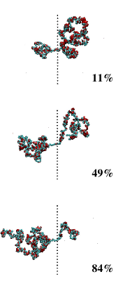
Figure 1: Snapshots of a typical event: a polymer ($N_{0}=300$) translocating from the right to the left is depicted at various stages of the process. The numbers shown in each panel represent the fraction of the polymer that has already passed through the pore. The vertical dots in the middle of each panel represent the membrane wall.

The variety of different initial polymer realizations produce a scaling law dependence of the translocation times on length Nelson . We construct duration histograms by accumulating all events for each length. The resulting distributions deviate from simple gaussians and are skewed towards longer times (see Fig. 2). Hence, the translocation time for each length is not assigned to the mean, but to the most probable time, which is the position of the maximum in the histogram. By calculating the most probable times for each length, a superlinear relation between the translocation time $\tau$ and the number of beads $N_{0}$ is obtained, as shown in Fig. 2(inset). The exponent in the scaling law $\tau(N_{0})\sim N_{0}^{\alpha}$ is calculated to be $\alpha\sim 1.28\pm 0.01$, for lengths up to $N_{0}=500$ beads. The observed exponent is in very good agreement with a recent experiment on double-stranded DNA translocation, that reported $\alpha\simeq 1.27\pm 0.03$ NANO . This agreement makes it plausible that the generic polymers modeled in our simulations can be thought of as DNA molecules. Without hydrodynamics translocation is significantly slowed down as indicated by a scaling exponent $\alpha^{\prime}\sim 1.36\pm 0.03$; data without the presence of a solvent are also presented in Fig. 2.

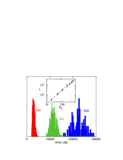
Figure 2: Duration histograms for polymers of different lengths. The distributions are skewed and the most probable time from these distributions is used to construct the scaling shown in the inset (cyan points). The scaling for the case without a fluid solvent is also shown (black points).

IV.2 Translocation dynamics

We next turn to the dynamics of the biopolymer as it passes through the pore. A radius of gyration $R_{I}(t)$ (with $I=U,T$) is assigned to each part of the polymer, the untranslocated and translocated one; we can also define an effective radius through

$$R_{eff}=\left[R_{T}^{\nu}+R_{U}^{\nu}\right]^{1/\nu}$$ (23)

with $\nu\sim 0.6$, which applies to a self-avoiding random walk. At the end of the translocation process, the radius of gyration is considerably smaller than it was initially: $R_{T}(t_{X})<R_{U}(0)$, where $t_{X}$ is the total translocation time for an individual event. Taking averages over a few hundreds of events for $N_{0}=200$ beads showed that $\lambda_{R}=R_{T}(t_{X})/R_{U}(0)\sim 0.7$. This reveals that as the polymer passes through the pore it becomes more compact than it was at the initial stage of the event, due to incomplete relaxation. In Fig. 3, we represent both radii of gyration as functions of the number of beads and of the translocation time. The curves shown in the figure are averages over about 100 events for $N_{0}=300$. By definition, $R_{U}(t)$ vanishes at $t=t_{X}$, while $R_{T}$ increases monotonically from $t=0$ up to $t=t_{X}$, although it never reaches the value $R_{U}(t=0)$. The rates of change of the two radii are approximately equal and constant (see left panel of Fig. 3), except at the end points of the event where the radius of gyration itself is not a well defined quantity because of the small number of beads included. The effective radius $R_{eff}$ shows a very small decreasing slope, in other words, it is almost constant (right panel of Fig. 3).

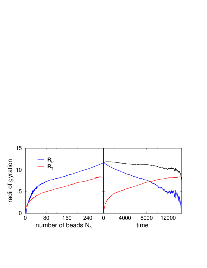
Figure 3: Radii of gyration as functions of the number of beads (left panel) and time (right panel) as an average over about 100 events for $N_{0}=300$. Blue is the untranslocated part $R_{U}$, red the translocated part $R_{T}$ and black the effective radius $R_{eff}$, defined in Eq. (23).

Throughout its motion the polymer continuously interacts with the fluid environment. The forces that essentially control the process are the electric drive $\vec{F}_{drive,i}$ and the hydrodynamic drag $\vec{F}_{drag,i}$ which act on each bead, for the untranslocated ($l=U$) and translocated ($l=T$) parts.. The drag forces $\vec{F}_{drag,i}$ on both parts of the polymer, change in time. In Fig. 4, both drag forces are presented as a function of time, together with their sum and the value of the electric drive in the pore, $F_{drive}=qE\langle N_{r}\rangle$, where $\langle N_{r}\rangle$ is the average number of resident monomers in the pore (simulations provide $N_{r}\sim 4.2$). This figure, referring to an average over the entire ensemble of trajectories for a $300$-monomer molecule, shows that the untranslocated strand alone can by no means balance the external force; only the sum of the translocated and untranslocated drag forces comes close to balancing the drive.

Apart from these forces and specifically at the end points (initiation and completion of the passage through the pore) entropic forces become important. The fluctuations experienced by the polymer due to the presence of the fluid are correlated to these entropic forces which, at least close to equilibrium, can be expressed as the gradient of the free energy with respect to the fraction of translocated beads. At the final stage of a translocation event, the radius of the untranslocated part undergoes a visible deceleration (see Fig. 3), the majority of the beads having already translocated. It is, thus, entropically more favorable to complete the passage through the hole rather than reverting it, that is, the entropic forces cooperate with the electric field and the translocation is accelerated.

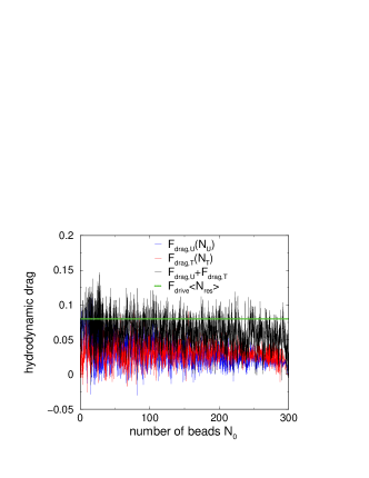
Figure 4: Viscous drag on the untranslocated and translocated parts of the polymer as a function of the number of beads and for an average of 100 translocations events with $N_{0}=300$ beads. The horizontal line denotes the electric drive in the pore region.

The entropic forces can also lead to rare events, such as retraction, which occur in our simulations at a rate less than 2% and depend on length, initial polymer configuration and parameter set. A retraction event is related to a polymer that anti-translocates after having partially passed through the pore. We have visually inspected the retraction events and associate them with the translocated part entering a low-entropy configuration (hairpin-like) subject to a strong entropic pull-back force from the untranslocated part: The translocated part of the polymer assumes an elongated conformation, which leads to an increase of the entropic force from the coiled, untranslocated part of the chain. As a result, the translocation is delayed and eventually the polymer is retracted.

IV.3 Translocation work

As a final step, we study the work performed on the biopolymer throughout its translocation. On general grounds, hydrodynamic interactions are expected to minimize frictional effects and form a cooperative background that assists the passage of the polymer through the pore. We investigate the cooperativity of the hydrodynamic field through the work ($W_{H}$) made by the fluid on the polymer per unit time:

$$\frac{dW_{H}}{dt}=\gamma\Big{\langle}\sum_{i}^{N_{0}}\vec{v}_{i}(t)\cdot\vec{u}_{i}(t)\Big{\rangle}$$ (24)

Through this definition, positive values of this hydrodynamic work rate indicate a cooperative effect of the solvent, while negative values indicate a competitive effect by the solvent. The work $W_{E}$ done per timestep by the electric field on the polymer can also be easily obtained through the expression:

$$\frac{dW_{E}}{dt}=\Big{\langle}\sum_{i}^{N_{0}}\vec{F}_{drive,i}\cdot\vec{v}_{i}(t)\Big{\rangle}$$ (25)

The brackets in the above equations denote averages over different realizations of the polymer for the same length. The results for the averages over all realizations are qualitatively similar to the work rates for an individual event of the same length. For all lengths studied here, we found that the total work per timestep of the hydrodynamic field on the whole chain is essentially constant, as shown in Fig. 5 for the averages over all events at each polymer length. For all these cases, the electric work rates are also constant with time. The hydrodynamic work per time is larger than the corresponding electric field work, because the latter only acts in the small region around the pore, and this is the reason why the electric field work is independent of polymer length.

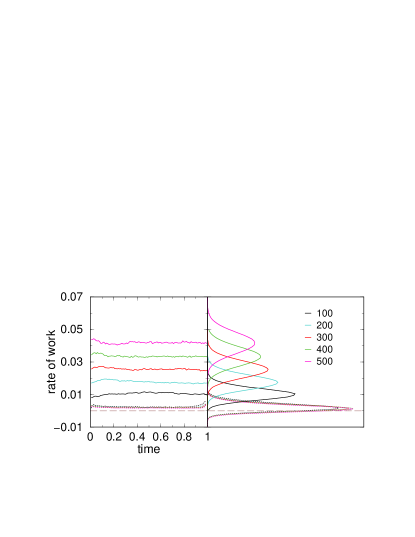
Figure 5: Translocation work per unit time for the hydrodynamic (solid lines) and electric fields (dotted lines) for polymers of different lengths. The right panel shows the probability distributions of both work rates. The labels correspond to the number of monomers $N_{0}$ for each case.

In addition to the variation of the work rates with time it is useful to analyze their distributions during translocation events. We show these in Fig. 5, where it is evident that the distribution of the hydrodynamic work rate lies entirely in the positive range, indicating that hydrodynamics turns the solvent into a cooperative environment, that is, it enhances the speed of the translocation process. In the same figure, the distribution for the electric work rate over all events for all lengths considered is also shown; these distributions are mostly positive but have a small negative tail which indicates that beads can be found moving against the electric field.

V Conclusions

We have presented a new multiscale methodology based on the direct coupling between atomic or molecular scale particle motion and mesoscopic hydrodynamics of the surrounding solvent. Due to the particle-like nature of the mesoscopic lattice Boltzmann solver, this coupling proceeds seamlessly in space and time. Correlations between the atomic scale and the hydrodynamic scale are also explicitly included through direct and local interactions between the particles representing solvent motion and the those belonging to the polymer. As a result, hydrodynamic interactions between the polymer and the surrounding fluid are explicitly taken into account, with no need of resorting to non-local representations. This allows a state-of-the-art modeling of biophysical phenomena, where hydrodynamic correlations play a significant role. We have also described an efficient parallel implementation of the method which exhibits excellent scalability on the IBM BlueGene platform.

As an application we modelled the translocation of polymers, which resemble DNA, through nanometer-sized pores. Besides statistical properties, such as scaling exponents, the present methodology affords direct insights into the details of the dynamics as well as the energetics of the translocation process, thereby offering a very valuable complement to experimental investigations of these complex and fascinating biological phenomena. It also shows a significant potential to deal with problems that combine complex fluid motion and dynamics at the molecular scale.

Acknowledgments

MF acknowledges support by Harvard’s Nanoscale Science and Engineering Center, funded by NSF (Award No. PHY-0117795). MB, SS and SM wish to thank the Initiative for Innovative Computing of Harvard University for financial support and the Harvard Physics Department and School of Engineering and Applied Sciences for their hospitality.

References

- (1) Lu, G. and Kaxiras, E.: Overview of Multiscale Simulations of Materials, Handbook of Theoretical and Computational Nanothechnology , Vol. X:1-33, edited by M. Rieth and W. Schommers, American Scientific Publishers, 2005.
- (2) Benzi, R. Succi, S., and Vergassola, M., Phys. Rep. 222:145-197, 1992.
- (3) D.A. Wolf–Gladrow, Lattice gas cellular automata and lattice Boltzmann models, Springer Verlag, New York, 2000.
- (4) Succi, S., The lattice Boltzmann equation. Oxford University Press, Oxford, 2001.
- (5) Fyta, M.G., Melchionna, S., Kaxiras, E., and Succi, S.: Multiscale coupling of molecular dynamics and hydrodynamics: application to DNA translocation through a nanopore. Multiscale Model. Simul. 5:1156-1173, 2006.
- (6) Ahlrichs, P. and Duenweg, B.: Lattice-Boltzmann simulation of polymer-solvent systems. Int. J. Mod. Phys. C 9:1429-1438, 1999; Simulation of a single polymer chain in solution by combining lattice Boltzmann and molecular dynamics. J. Chem. Phys. 111:8225-8239, 1999.
- (7) Adhikari, R., Stratford, K., Cates, M.E. and Wagner, A.J.: Fluctuating Lattice-Boltzmann, Europhys.Lett. 71:473-477, 2005.
- (8) Lodish, H., Baltimore, D., Berk, A., Zipursky, S., Matsudaira, P., and Darnell, J.: Molecular Cell Biology, W.H. Freeman and Company, New York, 1996.
- (9) Kasianowicz, J.J., et al: Characterization of individual polynucleotide molecules using a membrane channel. Proc. Nat. Acad. Sci. USA 93:13770-13773, 1996; Meller, A., et al: Rapid nanopore discrimination between single polynucleotide molecules. Proc. Nat. Acad. Sci. USA 97:1079-1084, 2000; Li, J., et al: DNA molecules and configurations in a solid-state nanopore microscope. Nature Mater. 2:611-615, 2003.
- (10) Sung, W. and Park, P. J.: Polymer translocation through a pore in a membrane. Phys. Rev. Lett. 77:783-786, 1996.
- (11) Matysiak, S., et al: Dynamics of polymer translocation through nanopores: Theory meets experiment. Phys. Rev. Lett. 96:118103, 2006.
- (12) Lubensky, D. K. and Nelson, D. R.: Driven polymer translocation through a narrow pore. Biophys. J. 77:1824-1838, 1999.
- (13) Ciccotti, G. and Ryckaert, J.-P.,: Molecular dynamics simulation of rigid molecules. Comp. Phys. Rep. 4:345-392, 1986.
- (14) Melchionna, S.: Design of quasi-symplectic propagators for Langevin dynamics. J. Chem. Phys., in press, 2007.
- (15) Andersen, H.C.: Rattle: a velocity version of the SHAKE algorithm for molecular dynamics calculations. J. Comp.Phys. 52:24-34, 1983.
- (16) Amati, G. Piva, R. and Succi, S.: Massively parallel Lattice-Boltzmann simulation of turbulent channel flow. Intl. J. Mod. Phys. C 4:869-877, 1997.
- (17) Boyer, L.L. Pawley, G.S.: Molecular dynamics of clusters of particles interacting with pairwise forces using a massively parallel computer. J. Comp. Phys. 78:405-423, 1988.
- (18) Heller, H. Grubmuller, H. Schulten, K.: Molecular dynamics simulation on a parallel computer. Molec. Sim. 5:133-165, 1990.
- (19) Rapaport, D.: Multi-million particle molecular dynamics: II.Design considerations for distributed processing. Comp.Phys.Comm. 62:198-216, 1991.
- (20) Brown, D. Clarke, J.H.R. Okuda, M. Yamazaki, T.: A domain decomposition parallelization strategy for molecular dynamics simulations on distributed memory machines. Comp.Phys.Comm. 74:67-80, 1993.
- (21) Esselink, K. Smit, B. Hilbers, P.A.J.: Efficient parallel implementation of molecular dynamics on a toroidal network: I.Parallelizing strategy. J. Comp. Phys. 106:101-107, 1993.
- (22) Plimpton, S.: Fast parallel algorithms for short-range molecular dynamics. J. Comp. Phys. 117:1-19, 1995.
-
(23)
http://domino.research.ibm.com/comm/research_projects.nsf/pages/bluegene.index.html - (24) Storm, A. J. et al: Fast DNA translocation through a solid-state nanopore. Nanolett. 5:1193-1197, 2005.