Self-induced oscillations in an optomechanical system

Abstract

We have explored the nonlinear dynamics of an optomechanical system consisting of an illuminated Fabry-Perot cavity, one of whose end-mirrors is attached to a vibrating cantilever. Such a system can experience negative light-induced damping and enter a regime of self-induced oscillations. We present a systematic experimental and theoretical study of the ensuing attractor diagram describing the nonlinear dynamics, in an experimental setup where the oscillation amplitude becomes large, and the mirror motion is influenced by several optical modes. A theory has been developed that yields detailed quantitative agreement with experimental results. This includes the observation of a regime where two mechanical modes of the cantilever are excited simultaneously.

Micro- and nanomechanical systems have become a focus of both theoretical and experimental research (Schwab and Roukes, 2005), with the goals ranging from ultrasensitive measurements to fundamental tests of quantum mechanics. One particularly promising branch of this field deals with optomechanical systems, where the interaction of light (stored inside an optical cavity) with macroscopic mechanical degrees of freedom (such as the coordinate of a cantilever) is exploited. This can give rise to a variety of effects, including a modification of the mechanical spring constant (Braginsky and Manukin, 1967; Vogel et al., 2003; Höhberger-Metzger and Karrai, 2004a; Arcizet et al., 2006; Corbitt et al., 2007), bistability (Dorsel et al., 1983; Meystre et al., 1985), optomechanical cooling, and parametric instability. A recent series of experiments has demonstrated impressive progress with respect to cooling (Höhberger-Metzger and Karrai, 2004b; Kleckner and Bouwmeester, 2006; Arcizet et al., 2006; Gigan et al., 2006; Schliesser et al., 2006; Corbitt et al., 2007; Favero et al., 2007; Thompson et al., 2007), which may ultimately lead to the quantum ground state (Marquardt et al., 2007; Wilson-Rae et al., 2007) of mechanical motion in such devices. On the other hand, the opposite regime is of equal interest, where the mechanical $Q$ factor is enhanced since the mechanical degree of freedom extracts energy provided by the optical radiation. In that regime, a parametric instability arises which drives the system into a state of self-sustained oscillations (Braginsky and Manukin, 1967; Braginsky et al., 1970, 2001; Kim and Lee, 2002; Höhberger and Karrai, 2004; Carmon et al., 2005; Kippenberg et al., 2005; Marquardt et al., 2006; Corbitt et al., 2006; Carmon and Vahala, 2007). Moreover, it is now known that the physics of that regime also applies to other systems as diverse as an LC circuit driven by a radio-frequency source (Brown et al., 2007) or a current-biased superconducting single-electron transistor coupled to a nanobeam (Naik et al., 2006; Rodrigues et al., 2007). Although the basic instability has been observed by now in a number of experiments (Kim and Lee, 2002; Höhberger and Karrai, 2004; Carmon et al., 2005; Kippenberg et al., 2005; Corbitt et al., 2006; Carmon and Vahala, 2007), it was recently realized theoretically (Marquardt et al., 2006) that the nonlinear dynamics of this system can become highly nontrivial, leading to an intricate attractor diagram. Here we report on an experiment that traces this diagram, and combine it with a detailed theoretical analysis and systematic quantitative comparison of theory and experiment. In addition, this comparison has enabled us to observe an unexpected feature, the simultaneous excitation of several mechanical modes of the cantilever, leading to coupled nonlinear dynamics.

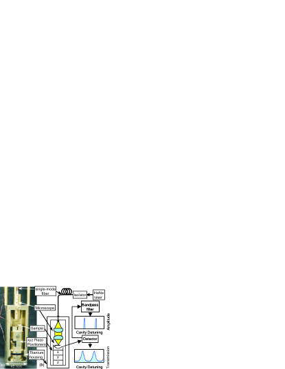
Figure 1: (Color online) The experimental setup. The light inside the optical cavity is focused onto a cantilever, where it exerts a force. Both the average transmitted light and its sidebands at the cantilever frequency are recorded (“Transmission” and “Amplitude”, respectively).

Experimental setup. - To study these questions, we employ the optomechanical setup displayed in Fig. 1. The light of a $633\,{\rm nm}$ monomode HeNe-laser is coupled into a single mode fiber and passes through a Faraday isolator (35 dB suppression). The fiber end inside a vacuum chamber (at $5\cdot 10^{-6}\,{\rm mbar}$) was polished and coated with a reflecting gold layer of $30\,{\rm nm}$ (yielding a theoretical reflectivity of $70\%$) to form the first cavity mirror. The sample is a gold-coated AFM cantilever acting as a micromirror, with length 223 $\mu$m, thickness 470 nm, width 22 $\mu$m, spring constant $K=0.01\,{\rm N/m}$, and a gold layer of $42\,{\rm nm}$ evaporated on one side only. The cantilever’s fundamental mechanical mode has a frequency of $\omega_{1}=2\pi\cdot 8.7\,{\rm kHz}$ and a damping rate of $\Gamma_{1}=30\,{\rm Hz}$. A simulation of the silicon-gold bilayer system gave a reflectivity of 91$\%$ for a wavelength of 633 nm. The divergent beam coming out of the fiber is sent through a microscope setup consisting of two identical lenses, yielding a Gaussian focus on the sample with a $1/e^{2}$-diameter of $6\,\mu{\rm m}$. The cantilever has been mounted on an $xyz$ piezo stepper positioner block , such that it can be placed at the microscope’s focal point, which was chosen near the end of the cantilever, at about 3/4 of its length. The finesse of the cavity defined by the sample and the fiber end was found to be $F\approx 4.5$. The transmitted intensity is measured with a Si photodiode behind the cantilever, while sweeping the cantilever position through the optical resonance.

Theoretical model. - The dynamics of the cantilever is described by the equation of motion of a damped oscillator, driven by light-induced forces:

$$\ddot{x}=-\omega_{1}^{2}(x-x_{0})-\Gamma_{1}\dot{x}+(F^{{\rm rad}}+F^{{\rm bol}})/m_{1}$$ (1)

Here $x(t)$ is the cantilever deflection observed at the laser spot. For now, we focus on the motion of the first mechanical mode (with effective mass $m_{1}$, frequency $\omega_{1}$, and damping rate $\Gamma_{1}$), and we will return to the influence of higher-order modes below. The cavity is assumed to be in resonance with the laser when $x=0$, while the mechanical equilibrium position is given by $x_{0}$ (sometimes referred to as the ’detuning’). In the experiment, it is controlled by the piezo positioning system. The radiation pressure force $F^{{\rm rad}}$ is proportional to the power $I$ circulating inside the cavity, $F^{{\rm rad}}/m_{1}=\mathcal{P}\cdot I$. The bolometric force $F^{{\rm bol}}$ arises due to light being absorbed, thus heating the cantilever that then deforms as a bimorph. It is enhanced by a factor $\Lambda$ over $F^{{\rm rad}}$ and is retarded due to the finite time of thermal conductance $\tau$:

$$F^{{\rm bol}}/m_{1}=\Lambda\mathcal{P}\int_{-\infty}^{t}\frac{dt^{\prime}}{\tau}e^{-(t-t^{\prime})/\tau}I(t^{\prime})\equiv\Lambda\mathcal{P}\theta(t).$$ (2)

Here $\theta$ is proportional to the change in temperature brought about by absorption of light.

We restrict the following discussion to the case of an optical ring down time that is much smaller than the period of cantilever oscillations (like in the present setup). Thus, the light intensity reacts instantaneously to the cantilever motion, $I(t)=I[x(t)]$. Due to the small finesse, we have to employ the Airy function dependence describing a series of overlapping Fabry-Perot resonances:

$$\frac{I[x(t)]}{I_{{\rm max}}}=\frac{1}{1+(2F/\pi)^{2}\sin(\frac{2\pi}{\lambda}x(t))^{2}}.$$ (3)

Here $I_{{\rm max}}$ is the peak circulating power, which is proportional to the input power. In contrast to the theory in (Marquardt et al., 2006), where a large optical ringdown time led to intensity oscillations, here the nonlinear dynamics is induced by the time retardation of the bolometric force.

Self-induced oscillations. - Time-retarded forces induce an effective optomechanical damping rate whose sign changes when passing through the resonance (Braginsky and Manukin, 1967; Braginsky et al., 1970; Höhberger-Metzger and Karrai, 2004a; Marquardt et al., 2006, 2007; Wilson-Rae et al., 2007). When the full damping rate becomes negative, the system undergoes a Hopf bifurcation and the cantilever settles into stable oscillations (Marquardt et al., 2006) which (for the parameters of interest here) are sinusoidal to a very good approximation: $x(t)=\bar{x}+A\cos(\omega_{1}t)$. The nonlinear dynamics can then be characterized by solving for the amplitude $A$ and offset $\bar{x}$. From these, it will be possible to obtain the experimentally observed evolution of the light intensity $I(t)$. In steady state, the average force and power input must be zero, i.e. $\left\langle\ddot{x}\right\rangle=0$ and $\left\langle\ddot{x}\dot{x}\right\rangle=0$, where $\left\langle\ldots\right\rangle$ denotes the time-average. Inserting Eq. (1), we obtain the power balance equation:

$$\mathcal{P}\left\langle\dot{x}(I(t)+\Lambda\theta(t))\right\rangle=\Gamma_{1}\left\langle\dot{x}^{2}\right\rangle\,.$$ (4)

The radiation pressure does not contribute, $\left\langle\dot{x}I\right\rangle=0$, since the intensity follows the motion instantaneously (thus $\dot{x}I$ is an antisymmetric function of time). The expression $\left\langle\dot{x}\theta\right\rangle$ may be simplified by introducing the first harmonic of the light intensity, $\tilde{I}_{1}=\frac{1}{T}\int_{0}^{T}dt\,\cos(\omega_{1}t)I(t)$ (with the period of mechanical motion $T=2\pi/\omega_{1}$):

$$\left\langle\dot{x}\theta\right\rangle=-A\omega_{1}\cdot\tilde{I}_{1}\frac{\omega_{1}\tau}{(\omega_{1}\tau)^{2}+1}\,.$$ (5)

This yields the first of the equations needed to find $\left(\bar{x},A\right)$:

$$\frac{\Gamma_{1}}{\mathcal{P}}=\frac{-\Lambda}{A\omega_{1}\pi}\frac{\omega_{1}\tau}{(\omega_{1}\tau)^{2}+1}\int_{0}^{2\pi}d\varphi\,I[\bar{x}+A\cos\varphi]\cos\varphi$$ (6)

Moreover, the force balance condition

$$\omega_{1}^{2}(\bar{x}-x_{0})=\mathcal{P}\cdot\left(\left\langle I\right\rangle+\Lambda\left\langle\theta\right\rangle\right)$$ (7)

enables us to obtain $\bar{x}=\bar{x}(x_{0},A)$:

$$\bar{x}-x_{0}=\frac{(1+\Lambda)\mathcal{P}}{2\pi\omega_{1}^{2}}\int_{0}^{2\pi}d\varphi\,I[\bar{x}+A\cos\varphi].$$ (8)

As a special case, for $A=0$, this contains the physics of static optomechanical bistability (Dorsel et al., 1983; Meystre et al., 1985).

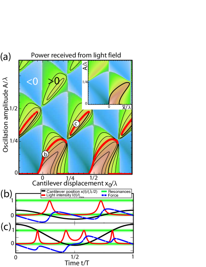
Figure 2: (Color online). Theoretically predicted attractor diagram for the nonlinear cantilever dynamics. (a) Amplitude $A$ of optomechanically induced oscillations vs. equilibrium position $x_{0}$ of the cantilever. The colorscale plot displays the net power fed into the cantilever from the radiation field, i.e. the r.h.s. of Eq. 6. Contour lines indicate possible oscillation amplitudes (dynamical attractors) for different values of the damping constant $\Gamma_{1}$. Red dots are the results of direct numerical simulations, for the value of $\Gamma_{1}$ realized in the present experimental setup (and a laser input power level of $I=0.3I_{0}$). The inset displays the same plot, but as a function of $(A,\bar{x})$ instead of $(A,x_{0})$, i.e. without the distortion due to the time-averaged radiation force that leads to $\bar{x}\neq x_{0}$. (b,c) Whenever the cantilever motion (thick black line) passes through the optical resonances (green bars), the light intensity (red line) displays spikes, which lead to delayed increases in the radiation force (dashed blue line), which was plotted as $(\theta-\bar{\theta})\times 200$. Plots (b) and (c) correspond to the respective positions indicated in the attractor diagram (a).

Attractor diagram. - Using Eqs. (6) and (8), one obtains solutions $(\bar{x},A)$ which can be visualized in attractor diagrams, like the one shown in Fig. 2. The color scale encodes the power input due to the light-induced forces (r.h.s. of Eq. 6), as a function of $x_{0}$ and $A$. The solution of Eq. 6 for various values of $\Gamma_{1}/\mathcal{P}$ then corresponds to contour lines of this function. Apart from the expected $\lambda/2$-periodicity in the detuning $x_{0}$, the main feature is the appearance of multiple solutions for $A$ at a given $x_{0}$ (“dynamical multistability”). Self-induced oscillations appear when $x(t)$ briefly dips into the resonance near its turning point, thereby gaining energy. Thus, to a first approximation, attractors appear along the diagonals $A\approx\bar{x}+n\lambda/2$. Near the special points $\bar{x}=\lambda/4+n\lambda/2$, the total power input vanishes due to symmetry: The cantilever extracts energy from the light field at one turning point but loses an equal amount of energy at the other turning point.

The deviation between $\bar{x}$ and $x_{0}$, obtained from Eq. (8), leads to a distortion of the diagram (compare inset of Fig. 2). This effect grows with increasing input power, finally leading to multiple solutions for $\bar{x}(x_{0},A)$.

Comparison of theory and experiment. - In the experiment, the detuning $x_{0}$ and the input power $I_{{\rm in}}$ are varied, while the transmitted light intensity is measured. This can be compared to the time-averaged circulating power $\left\langle I(t)\right\rangle$ obtained from the theory. Moreover, as soon as the self-induced oscillations set in, $I(t)$ is modulated at the cantilever frequency. A very helpful nontrivial feature of this system is the existence of a relation between the motional amplitude $A$ and the first harmonic of the light intensity, $\tilde{I}_{1}$ (defined above). From Eq. (6), we see that they are directly proportional, with the proportionality factor containing only known, fixed parameters: $A=-2(\Lambda\mathcal{P}/\omega_{1}\Gamma)\omega_{1}\tau(1+(\omega_{1}\tau)^{2})^{-1}\tilde{I}_{1}$. This relation holds true only in steady state (on the attractors), but then it is valid even when the motion sweeps across several optical resonances. Experimentally, the first harmonic $\tilde{I}_{1}$ is obtained by sending the photodetector signal through a narrow bandpass filter ($100\,{\rm Hz}$) centered at the eigenfrequency $\omega_{1}$ of the first mechanical mode.

Theoretical and experimental curves for both the average intensity (“transmission”) and the amplitude are shown in Fig. 3, for different input powers. For this comparison, the following parameters have been used: $F\approx 4.5$ (from a fit at low input power), $\Lambda=3950$ and $\omega_{1}\tau=39$ (obtained independently). The overall conversion factor between experimentally measured input power and the force on the cantilever was found to be $\mathcal{P}I_{{\rm 0}}=0.0775{\rm m/s^{2}}$, by adjusting for a good fit to the data at intermediate power (the same was done for the rescaling of theoretical and experimental transmission intensity). Here the maximum laser power $I_{0}=1.3\,{\rm mW}$ is estimated to yield $500\,\mu{\rm W}$ circulating in the cavity on resonance.

At the lowest power displayed in Fig. 3, self-oscillations have just set in, and the transmission curve shows a striking asymmetry. At higher input powers, the multistability predicted by the attractor diagram, Fig. 2, leads to hysteresis effects that appear upon sweeping $x_{0}$ up and down.

Beginning at $I_{{\rm in}}=0.57\,I_{0}$, a second interval of self-oscillatory behaviour appears to the left of the resonance, growing stronger and wider with increasing laser power. This initially completely unexpected result may be explained by invoking the influence of higher mechanical modes. These may be excited by the radiation as well, leading to coupled (multimode) nonlinear dynamics with richer features than discussed up to now.

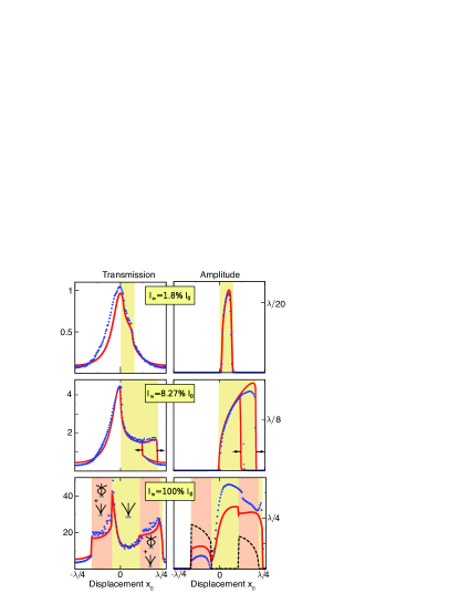
Figure 3: (Color online) Experiment vs. theory. The transmitted light intensity (left) and the amplitude of self-induced cantilever oscillations (right), from a simulation of the theoretical model (red full curves) and from the experiment (blue data points), at increasing input power levels (top to bottom). Theoretical “transmission” curves display the (rescaled) time-averaged circulating light intensity from the simulation. “Amplitude” curves are obtained from the power in the intensity sidebands at the fundamental mechanical mode of the cantilever (see main text). For clarity, the hysteresis observed upon sweeping $x_{0}$ up or down has been shown only in the middle panel. The region of instability (shaded interval) grows with increasing input power. Simultaneous self-induced oscillations of the first two mechanical modes set in at the highest power displayed (in the two intervals indicated in the plot). The calculated amplitude of the second mode is shown as a dashed line.

In order to describe the behaviour in that case, we now take into account the second mode as well. The total displacement is $x(t)=x_{0}+x_{1}(t)+x_{2}(t)$, and we have to employ a set of equations:

$$\ddot{x}_{i}=-\omega_{i}^{2}x_{i}-\Gamma_{i}\dot{x_{i}}+F_{i}^{{\rm bol}}[x(t)]/m_{i}\,,$$ (9)

where $x_{i}$ denotes the coordinate of the $i$-th mechanical mode with frequency $\omega_{i}$, mechanical damping rate $\Gamma_{i}$, and effective mass $m_{i}$ (where $\omega_{1}/2\pi=8.7\,{\rm kHz}$, $\omega_{2}/2\pi=60\,{\rm kHz}$, $\Gamma_{1}=30.0\,{\rm Hz}$, $\Gamma_{2}=150\,{\rm Hz}$). We neglected the radiation pressure force, as this is much smaller anyway for the parameters of this setup. The mechanical modes are now coupled indirectly by the bolometric force. For the present setup, this force changes sign when going to the second mode. Choosing $F_{2}^{{\rm bol}}m_{1}/F_{1}^{{\rm bol}}m_{2}=-28.8$ as an adjustable parameter, we have found the numerical simulation of these coupled nonlinear equations for the first two modes to be in surprisingly good agreement with the experiment (Fig. 3). We have to note that the relation between the measured “amplitude”, i.e. first harmonic of $I(t)$ at frequency $\omega_{1}$, and the actual amplitude $A_{1}$ does not hold exactly if both modes are excited simultaneously.

At maximum laser power, there are actually two intervals with simultaneous excitation of both modes (indicated in Fig. 3). Specifically, the onset of such a regime at $x_{0}\approx\lambda/8$ can be interpreted as follows: Taking into account $F_{2}^{{\rm bol}}/F_{1}^{{\rm bol}}<0$, we see that the second mode gains its energy from dipping into the resonance at $x=\lambda/2$, while the first is still provided with energy due to the resonance at $x=0$.

Numerical evidence shows that the steady-state motion consists of sinusoidal oscillations in $x_{1,2}$ at the respective eigenfrequencies, of nearly constant amplitudes and without phase locking (for the parameters explored here). Thus $x(t)\approx x_{0}+\sum_{i=1}^{2}[A_{i}+\delta A_{i}(t)]\cos(\omega_{i}t+\phi_{i})$, where $\delta A_{i}(t)/A_{i}\ll 1$, and the $\phi_{i}$ are arbitrary phases. Higher input powers will lead to excitations of additional modes, and the system might go into a chaotic regime of motion.

Conclusions. - We have analyzed the nonlinear dynamics of an optomechanical system, by measuring and explaining its attractor diagram. The comparison of data and theoretical predictions have revealed the onset of multi-mode dynamics at large optical power, with two mechanical modes of the cantilever participating in the radiation-driven self-sustained oscillations. These effects could find applications in highly sensitive force or displacement detection (Marquardt et al., 2006). In the future, it would be interesting to observe the attractor diagram in systems of a high optical finesse (Carmon et al., 2005; Kippenberg et al., 2005) (with delayed radiation dynamics), or the self-excitation of multiple mechanical modes of sub-wavelength mechanical resonators interacting with the radiation field inside a cavity (Favero and Karrai, 2007; Thompson et al., 2007). The whole field of quantum nonlinear dynamics in systems of this kind also remains to be explored.

We acknowledge support by the Nanosystems Initiative Munich (NIM). F. M. acknowledges support by an Emmy-Noether grant of the DFG, and I. F. acknowledges the A. v. Humboldt Foundation.

* Note: The first two authors (M. L. and C. N.) contributed equally to this work.

References

- Schwab and Roukes (2005) K. C. Schwab and M. L. Roukes, Physics Today July Issue, 36 (2005).
- Braginsky and Manukin (1967) V. Braginsky and A. Manukin, Soviet Physics JETP 25, 653 (1967).
- Vogel et al. (2003) M. Vogel, C. Mooser, K. Karrai, and R. J. Warburton, Applied Physics Letters 83, 1337 (2003).
- Höhberger-Metzger and Karrai (2004a) C. Höhberger-Metzger and K. Karrai, Nature 432, 1002 (2004a).
- Arcizet et al. (2006) O. Arcizet, P. F. Cohadon, T. Briant, M. Pinard, and A. Heidmann, Nature 444, 71 (2006).
- Corbitt et al. (2007) T. Corbitt et al., Phys. Rev. Lett. 98, 150802 (2007).
- Dorsel et al. (1983) A. Dorsel, J. D. McCullen, P. Meystre, E. Vignes, and H. Walther, Phys. Rev. Lett. 51, 1550 (1983).
- Meystre et al. (1985) P. Meystre, E. M. Wright, J. D. McCullen, and E. Vignes, J. Opt. Soc. Am. B 2, 1830 (1985).
- Höhberger-Metzger and Karrai (2004b) C. Höhberger-Metzger and K. Karrai, Nature 432, 1002 (2004b).
- Kleckner and Bouwmeester (2006) D. Kleckner and D. Bouwmeester, Nature 444, 75 (2006).
- Gigan et al. (2006) S. Gigan et al., Nature 444, 67 (2006).
- Schliesser et al. (2006) A. Schliesser, P. Del’Haye, N. Nooshi, K. J. Vahala, and T. J. Kippenberg, Phys. Rev. Lett. 97, 243905 (2006).
- Favero et al. (2007) I. Favero et al., Applied Physics Letters 90, 104101 (2007).
- Thompson et al. (2007) J. D. Thompson, B. M. Zwickl, A. M. Jayich, F. Marquardt, S. M. Girvin, and J. G. E. Harris, arXiv:0707.1724 (2007).
- Marquardt et al. (2007) F. Marquardt, J. P. Chen, A. A. Clerk, and S. M. Girvin, Phys. Rev. Lett. 99, 093902 (2007).
- Wilson-Rae et al. (2007) I. Wilson-Rae, N. Nooshi, W. Zwerger, and T. J. Kippenberg, Phys. Rev. Lett. 99, 093901 (2007).
- Braginsky et al. (1970) V. B. Braginsky, A. B. Manukin, and M. Y. Tikhonov, Soviet Physics JETP 31, 829 (1970).
- Braginsky et al. (2001) V. B. Braginsky, S. E. Strigin, and S. P. Vyatchanin, Physics Letters A 287, 331 (2001).
- Kim and Lee (2002) K. Kim and S. Lee, Journal of Applied Physics 91, 4715 (2002).
- Höhberger and Karrai (2004) C. Höhberger and K. Karrai, Nanotechnology 2004, Proceedings of the 4th IEEE conference on nanotechnology p. 419 (2004).
- Carmon et al. (2005) T. Carmon, H. Rokhsari, L. Yang, T. J. Kippenberg, and K. J. Vahala, Phys. Rev. Lett. 94, 223902 (2005).
- Kippenberg et al. (2005) T. J. Kippenberg, H. Rokhsari, T. Carmon, A. Scherer, and K. J. Vahala, Phys. Rev. Lett. 95, 033901 (2005).
- Marquardt et al. (2006) F. Marquardt, J. G. E. Harris, and S. M. Girvin, Phys. Rev. Lett. 96, 103901 (2006).
- Corbitt et al. (2006) T. Corbitt et al., Phys. Rev. A 74, 021802 (2006).
- Carmon and Vahala (2007) T. Carmon and K. J. Vahala, Phys. Rev. Lett. 98, 123901 (2007).
- Brown et al. (2007) K. R. Brown, J. Britton, R. J. Epstein, J. Chiaverini, D. Leibfried, and D. J. Wineland, Phys. Rev. Lett. 99, 137205 (2007).
- Naik et al. (2006) A. Naik et al., Nature 443, 193 (2006).
- Rodrigues et al. (2007) D. A. Rodrigues, J. Imbers, T. J. Harvey, and A. D. Armour, New Journal of Physics 9, 84 (2007).
- Favero and Karrai (2007) I. Favero and K. Karrai, arXiv:0707.3117 (2007).