Spontaneous breaking of translational invariance in non-commutative $\lambda\phi^{4}$ theory in two dimensions.

Abstract

The spontaneous breaking of of translational invariance in non-commutative self-interacting scalar field theory in two dimensions is investigated by effective action techniques. The analysis confirms the existence of the stripe phase, already observed in lattice simulations, due to the non-local nature of the non-commutative dynamics.

The existence of a phase with conventional long range order, or spontaneous symmetry breaking (SSB) for two dimensional (2D) systems with continuous symmetry group, is precluded by the Coleman-Mermin-Wagner (CMW) theorem, which has been formulated specifically for spin models in mermin and for quantum fields in coleman . In these low-dimensional systems the infrared divergences related to the spin waves or Goldstone modes are so strong that the long range order is destroyed, so that the typical order parameter (or scalar field expectation value) vanishes. However, in 2D, as for instance in the XY model, it is still possible to have a Kosterlitz-Thouless phase transition kt driven by the presence of topological defects and a quantum field theory which displays an “almost” long range order witten .

For quantum fields, the CMW theorem relies on the hypotesis of locality. In fact there are known exceptions such as the Liouville theory roman1 ; lautrup . Another interesting case which is certainly relevant for this problem is the non-commutative formulation of the quantum field theory because in this framework the above hypotesis is not respected.

In the non-commutative theory the canonical commutator among space-time coordinates is

$$[x_{\mu},x_{\nu}]=i\theta_{\mu\nu},$$ (1)

and the product of field operators is non-local, being defined by the Moyal product connes . For example for the scalar $\lambda\phi^{4}$ theory the non-commutative interaction lagrangian is

$$L_{I}={\lambda\over 4!}\phi^{4*}$$ (2)

where the Moyal (star) product is defined by ($i,j=1,.,4$) connes

$$\phi^{4*}(x)=\phi(x)*\phi(x)*\phi(x)*\phi(x)=\exp\left[{i\over 2}\sum_{i<j}\theta_{\mu\nu}\partial^{\mu}_{x_{i}}\partial^{\nu}_{x_{j}}\right]\Bigl{(}\phi(x_{1})\phi(x_{2})\phi(x_{3})\phi(x_{4})\Bigr{)}\left|{}_{x_{i}=x}\right.$$ (3)

The Moyal product induces an infrared-ultraviolet (IR-UV) connection which deeply modifies the structure of the theory with respect to the commutative case. In fact, it is still unclear whether a consistent non-commutative field theory exists in the continuum limit although recent lattice simulations suggest that a consistent non-commutative $U(1)$ gauge theory can be defined bietenolzzero , with possible phenomenological implications noizero ; alt ; urru ; hin .

An interesting aspect of non-commutative scalar theories is that, in 4D, SSB is possible only in an inhomogeneous phase , i.e. where the vacuum expectation value of the field is position-dependent gubser . This phase is called the stripe phase for the peculiar $x$ dependence of the order parameter $<\Phi(x)>_{0}$. This unexpected result, conjectured and discussed on the basis of the IR-UV connection in gubser , has then been obtained by an effective action technique noi ; romano and confirmed by lattice simulations bietenolz1 .

The stripe phase involves the spontaneous breaking of translational invariance which, in 2D, should be forbidden according to the CMW theorem. Gubser and Sondhi gubser , on the basis of a Brazovski-like local effective lagrangian braz which is quartic in momentum and represents a good description of the non-commutative effects near the minimum of the particle self-energy, generated by the IR-UV connection, exclude the 2D stripe phase, in agreement with the CMW theorem. Indeed, they find that the infrared behavior of the 2D non-commutative theory is even more pathological than that observed in the commutative case.

On the other hand, it has been reported in catterall that, in 2D lattice simulations of non-commutative scalar $\lambda\phi^{4}$ theory, the translational invariance is spontaneously broken and another numerical experiment, bietenolz2 , with a more efficient algorithm, essentially confirms the existence of the 2D stripe phase. Therefore the validity of the CMW theorem for non-commutative theories is still under investigation and in this letter we carry on this analysis, by resorting to the same functional technique already used in noi , which corresponds to an Hartree-Fock computation of the effective action. Within this approach which, in the commutative case, confirms the validity of the CMW theorem poli , and according to the approximations considered in the following, it is shown that the stripe phase exists also in 2D, due to non-commutativity.

By following noi , let us first verify that, for non-commutative $\lambda\phi^{4}$ theory in 2D there is no spontaneous symmetry breaking with a constant order parameter. The action is

$$I(\phi)=\int d^{2}x\left({1\over 2}\partial_{\mu}\phi~{}\partial^{\mu}\phi-{1\over 2}m^{2}\phi^{2}-{\lambda\over 4!}\phi^{4*}\right)$$ (4)

and, by assuming a translational invariant propagator

$$G(x-y)=\int\frac{d^{2}p}{(2\pi)^{2}}\;\frac{e^{-ip(x-y)}}{p^{2}-M^{2}(p)}\;\;,$$ (5)

the Cornwall-Jackiw-Tomboulis cjt effective action in the Hartree-Fock approximation in momentum space is given by noi

$$\Gamma(\phi,G)={1\over 2}\int{d^{4}p\over{(2\pi)^{4}}}(p^{2}-m^{2})\phi(p)\phi(-p)$$

$$-{\lambda\over{4!}}\left[{\prod_{a=1}^{4}\int{d^{4}p_{a}\over{(2\pi)^{4}}}\phi(p_{a})}\right]\delta^{4}\left(\sum_{a}{p_{a}}\right)\exp\left({i\over 2}p_{1}\wedge p_{2}\right)\exp\left({i\over 2}p_{3}\wedge p_{4}\right)$$

$$+{i\over 2}\delta^{4}(0)\int{d^{4}p\over(2\pi)^{4}}\ln D(p)G^{-1}(p)+{1\over 2}\delta^{4}(0)\int{d^{4}p\over(2\pi)^{4}}(p^{2}-m^{2})G(p)$$

$$-{\lambda\over 6}\int{d^{4}p\over(2\pi)^{4}}\int{d^{4}q\over(2\pi)^{4}}\phi(p)\phi(-p)G(q)\left[1+{1\over 2}\exp{(iq\wedge p)}\right]$$

$$-{\lambda\over{12}}\delta^{4}(0)\int{d^{4}p\over(2\pi)^{4}}\int{d^{4}q\over(2\pi)^{4}}G(p)G(q)\left[1+{{1\over 2}}\exp{(iq\wedge p)}\right]$$ (6)

where $D(p)$ is the free propagator with mass $m$ and $q\wedge p=q_{\mu}\theta^{\mu\nu}p_{\nu}$.

In euclidean space the coupled minimization equations, $\delta\Gamma/\delta\phi=0$ and $\delta\Gamma/\delta G=0$, for a constant background $\phi_{0}$, can be written as

$$M^{2}(q)=\mu^{2}+\frac{\lambda}{2}\phi_{0}^{2}+\frac{\lambda}{3}I(\sigma)+\frac{\lambda}{6}\int\frac{d^{2}p}{(2\pi)^{2}}\frac{1}{p^{2}+M^{2}(p)}e^{iq\wedge p}$$ (7)

and

$$0=\phi_{0}\left(\frac{\lambda}{3}\phi_{0}^{2}-M^{2}(q)\right)\delta^{2}(q)$$ (8)

where, in eq. (7), the bare mass $m$ has been replaced by $\mu$, according to the renormalization :

$$m^{2}=\mu^{2}-\frac{\lambda}{3}\int\frac{d^{2}p}{(2\pi)^{2}}\frac{1}{p^{2}+\sigma^{2}},$$ (9)

and we have defined

$$I(\sigma)=\int\frac{d^{2}p}{(2\pi)^{2}}\left[\frac{1}{p^{2}+M^{2}(p)}-\frac{1}{p^{2}+\sigma^{2}}\right].$$ (10)

The parameter $\sigma$ has the role of infrared cut-off.

The non-commutative phase factor connects the infrared and ultraviolet regions and therefore one needs a self-consistent approach. Let us start by noting that , due to the strongly oscillating phase factor, for $q\to\infty$ the last integral in the right hand side of eq. (7) takes its contribution from the region $p\sim 0$ and therefore we can set

$${\rm lim}_{q\rightarrow\infty}M^{2}(q)\rightarrow M^{2}_{asy},$$ (11)

where the constant $M^{2}_{asy}$ does not depend on $q$, provided that

$$\int\frac{d^{2}p}{(2\pi)^{2}}\frac{1}{p^{2}+M^{2}(p)}$$ (12)

is finite (as we shall check self-consistently).

Then, in the infrared region (small $q$) where the mentioned integral gets contributions only from large values of the variable $p$, we can approximate $M^{2}(p)$ with its asymptotic value given in eq. (11) and we get

$${\rm lim}_{q\rightarrow 0}M^{2}(q)\simeq\mu^{2}+\frac{\lambda}{2}\phi_{0}^{2}+\frac{\lambda}{3}I(\sigma)+\frac{\lambda}{6}\int\frac{d^{2}p}{(2\pi)^{2}}\frac{1}{p^{2}+M^{2}_{asy}}e^{iq\wedge p}$$ (13)

For $\theta^{\mu\nu}$ of maximal rank and eigenvalues $\pm\theta$, it turns out gubser that

$$\int\frac{d^{2}p}{(2\pi)^{2}}\frac{1}{p^{2}+M^{2}_{asy}}e^{iq\wedge p}=\frac{1}{2\pi}K_{0}(M_{asy}|q|\theta)$$ (14)

where $K_{0}$ is the modified Bessel function which, for $|q|\rightarrow 0$, has the asymptotic behavior

$$K_{0}(M_{asy}|q|\theta)\rightarrow-{\rm ln}(M_{asy}|q|\theta/2)$$ (15)

Therefore , for any value of $\sigma$,

$${\rm lim}_{q\rightarrow 0}M^{2}(q)\simeq-{\rm ln}(M_{asy}|q|\theta/2)$$ (16)

which is inconsitent with the second minimization equation

$$M^{2}(0)=\frac{\lambda}{3}\phi_{0}^{2}$$ (17)

for any finite value of $\phi_{0}$ foot .

This shows that the class of solutions considered so far cannot fulfill the minimization equations derived above. The simplest generalization consists in releasing the constraint of a translationally invariant vacuum expectation value of the field which, as seen in noi provides a viable solution in the four-dimensional problem. In fact we look for solutions in the form of oscillating field

$$\phi(x)=A\;{\rm cos}(Q\cdot x)$$ (18)

where $A$ is a scalar and $Q$ a bidimensional vector, which would require a non-translational invariant full propagator $G$. However, as discussed in noi , a self-consistent approach in evaluating the effective action is obtained, for small $Q$, by a translational invariant ansatz ( see eq. (5) ) where, however, the function $M(p)$ takes into account the asymptotic, infrared and ultraviolet, behaviors of the gap equation with the non-uniform background. The standard homogeneous case, $Q=0$, is recovered by neglecting the non-commutative effects that is by considering the so called planar limit, $\theta\Lambda^{2}\rightarrow\infty$ , where $\Lambda$ is an ultraviolet cut-off. From this point of view a small $Q$ ( in cut-off units) is associated with large, but finite, values of $\theta\Lambda^{2}$ that we shall assume in the remaining part of the paper.

The constant $A$, the vector $Q$ and the momentum dependent mass $M(p)$ are the three parameters that must be determined by the extremization of the action in eq. (6). Without loss of generality we can choose a specific direction for the vector $Q$, e.g.: $Q_{1}=0,\;Q_{2}=Q$ and then the extremum equations for the action read:

$$M^{2}(q)=\mu^{2}+A^{2}{\lambda\over 6}\left(1+{1\over 2}\cos{(q_{1}\theta Q)}\right)+\frac{\lambda}{3}I(\sigma)+\frac{\lambda}{6}\int\frac{d^{2}p}{(2\pi)^{2}}\frac{\cos{[\theta(q_{1}p_{2}-q_{2}p_{1})]}}{p^{2}+M^{2}(p)}$$ (19)

$$A\left[Q^{2}+A^{2}{\lambda\over 8}+\mu^{2}+{\lambda\over 3}I(\sigma)++\frac{\lambda}{6}\int\frac{d^{2}p}{(2\pi)^{2}}\frac{\cos{(p_{1}\theta Q)}}{p^{2}+M^{2}(p)}\right]=0$$ (20)

$$Q^{2}-{\lambda\over 12}\int\frac{d^{2}p}{(2\pi)^{2}}\frac{(p_{1}\theta Q)\;\sin{(p_{1}\theta Q)}}{p^{2}+M^{2}(p)}=0$$ (21)

Since the self-consistent approach requires small $Q$ and in particular in the planar theory limit, i.e. for large $\theta$, $Q$ must approach zero in such a way that $\theta Q<<1$ ( in cut-off units), then in eq. (21) one can approximate $M^{2}(p)\simeq M^{2}_{asy}$ to obtain

$$Q^{2}=\frac{\lambda}{24\pi}M_{asy}\;\theta\;Q\;\;K_{1}(M_{asy}\theta Q)$$ (22)

where $K_{1}(x)$ is the modified Bessel function. Also by this semplification, there is no way to solve analitically the coupled equations for $A$ and $M(p)$ and therefore we consider a Raileigh-Ritz approach, i.e. a parametric ansatz for $M(p)$ and an evaluation of the effective action for different values of the parameters.

According to the previous analysis, the ansatz for $M(p)$ , consistent with the infrared and ultraviolet behaviors of the gap equation, is given by

$$M^{2}(p)=M^{2}_{0}-\frac{\lambda}{12\pi}\ln\left(\frac{|p|}{Q}\right)\phantom{......}|p|<Q$$ (23)

and

$$M^{2}(p)=M^{2}_{0}\phantom{....}|p|\geq Q$$ (24)

where $M_{0}$ is a constant. Therefore $Q$ is obtained by eq. (21) with $M_{asy}=M_{0}$.

We compute the effective action for the specific field configuration given in eq. (18) and subtract the constant corresponding to the same effective action evaluated at $A=0$, $M^{2}(p)=\sigma^{2}$ and $\theta\Lambda^{2}\to\infty$ (planar limit). In Figs.1 and 2 we plot the subtracted effective action $W$ as a function of $A$, for $\lambda=0.1$, $\theta=10$ , $\sigma=10^{-5}$ and, in Fig. 1, for $\mu^{2}=-0.1$ and three different values of $M_{0}$: 0.1, 0.34, 0.6, while in Fig. 2 for $\mu^{2}=0.1$ and $M_{0}$: 0.1, 0.22, 0.4 (with all dimensionful quantities expressed in units of the UV cutoff $\Lambda$). For the parameters $\theta$ and $M_{0}$ used in the figures, the corresponding value of $Q$, derived from eq. (22), is about $Q\sim 2.6\;10^{-2}$, which is consistent with the condition $\theta Q<<1$ in cut-off units, discussed above.

These examples show that for sufficiently negative $\mu^{2}$ a minimum of $W$ is observed at $A\neq 0$, whereas, by sufficiently increasing $\mu^{2}$ to positive values, the minimum of $W$ is shifted to $A=0$. In each figure we have plotted the effective action for three values of $M_{0}$, and the curves labelled with $(b)$ correspond to the optimal value $M_{0}$ which provides the lowest value of $W$. By reducing or increasing $M_{0}$ with respect to this optimal value, one finds that the minimum of $W$ is increased. We have checked that the behavior shown in the figures is stable against changes of the infrared regulator, i.e. for any value of $\sigma$ there is a value of $\mu^{2}$ below which the minimum of $W$ is located at $A\neq 0$. Furthermore, the structure displayed in Figs. 1 and 2 does not change when varying $\lambda$ and $\theta$ in a wide range of values.

This can also be partially shown analytically. Indeed, by handling the coupled minimum equations for $A$, $Q$ and $M(p)$: (19), (20) and (21), one can show that

$$\frac{\lambda}{8}A^{2}=Q^{2}+M^{2}(Q)$$ (25)

and therefore a solution exists if $M^{2}(Q)\geq 0$ , that is if the gap equation has a real solution.

Therefore, although it does not provide a formal proof, the previous analysis strongly supports the conclusion that the translational invariance is spontaneously broken for the non-commutative scalar field theory in 2D, i.e. there is a minimum of the effective potential for $A\neq 0$,$Q\neq 0$ and $M_{0}\neq 0$.

As recalled in the introduction a similar phenomenon occurs in the Liouville theory with lagrangian

$$L=\frac{1}{2}(\partial_{\mu}\phi)(\partial^{\mu}\phi)-\frac{m^{2}}{\beta^{2}}\exp\left(\beta\phi\right)$$ (26)

with $\beta>0$ and $m^{2}>0$. In roman1 it has been suggested that the spontaneous breakdown of spatial translational invariance occurs in this model and that one can build a consistent perturbation theory on a static, position-dependent background. Moreover the existence of these non-translationally invariant states has been tested by Montecarlo simulations lautrup .

In gubser the validity of CMW theorem for the non-commutative scalar theory in 2D has been shown for a complex scalar field, where the O(2) invariance implies zero modes, as seen by using the Brazovskii-like local effective lagrangian

$$L_{B}=\frac{1}{2}k_{1}|(\partial^{2}+p_{c}^{2})\phi|^{2}+\frac{1}{2}k_{2}\phi^{2}+\frac{1}{4}k_{4}\phi^{4}$$ (27)

where $k_{1},k_{4}>0$, $k_{2}<0$ and $p_{c}$ is the momentum where the self-energy has a minimum.

This effective lagrangian is a good approximation near the minimum and it is quartic in momentum. Therefore, if there are zero modes, the infrared behavior of the fluctuactions is worse than the standard 2D case, hence enforcing the validity of CMW theorem. However for a single scalar field the non-translationally invariant configuration that gives the zero modes, if any, is not easy to build and in this case there is no evidence that the CMW theorem is still valid.

In conclusion, our opinion is that the theoretical problem of the CMW theorem for non-commutative 2D theory is still open but, for a single scalar field and without considering an effective lagrangian, the indication given in this paper confirms the lattice results that the translational invariance is spontaneously broken due to the non-commutative dynamics.

Acknowledgement
The authors thank Roman Jackiw and So Young Pi for useful suggestions and comments. The work of PC has been supported by the “Bruno Rossi” program. PC is grateful to the Boston University for kind hospitality.

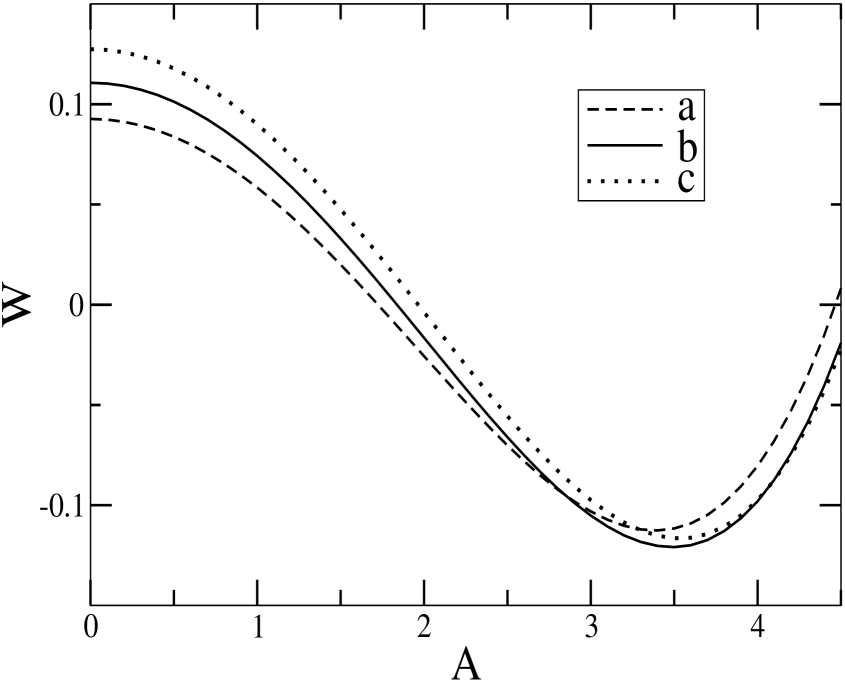
Figure 1: The normalized effective action for $\mu^{2}=-0.1$ and: (a) $M_{0}=0.1$, (b) $M_{0}=0.34$, (c) $M_{0}=0.6$.

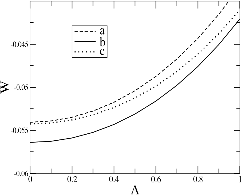
Figure 2: The normalized effective action for $\mu^{2}=0.1$ and: (a) $M_{0}=0.1$, (b) $M_{0}=0.22$, (c) $M_{0}=0.4$.

References

- (1) N.D. Mermin and H. Wagner, Phys. Rev. Lett. 17 (1966) 1133.
- (2) S. Coleman, Commun. Math. Phys. 31 (1973) 259.
- (3) J.M. Kosterlitz and D.J. Thouless, Jour. Phys. C6 (1973) 1181.
- (4) E. Witten, Nucl. Phys. B 145 (1978) 110.
- (5) E. D’Hoker and R. Jackiw, Phys. Rev. Lett. 50 (1983) 1719; Phys. Rev. D 26 (1982) 3517.
- (6) C. Bernard, B. Lautrup and E. Rabinovici, Phys. Lett. B 134 (1984) 335.
- (7) A. Connes, M.R. Douglas, A. Schwarz, JHEP 02 (1998) 003. For a review see M.R. Douglas, N.A. Nekrasov, Rev. Mod. Phys. 73 (2001) 977; R.J. Szabo, Phys. Rep. 378 (2003) 207.
- (8) W. Bietenholz et al. , JHEP 0610:042 (2006).
- (9) P. Castorina, A. Iorio and D. Zappalà, Europhys. Lett. 69 (2005) 912; Phys. Rev. D 69 (2004) 065008.
- (10) B. Altschul, Phys. Rev. D 72 (2005) 085003; Phys. Rev. Lett. 96 (2006) 201101.
- (11) R.Montemayor and L.F. Urrutia, Phys. Lett. B 606 (2005) 86.
- (12) I. Hinchliffe et al., Int. J. Mod. Phys. A 19 (2004) 179.
- (13) S.S. Gubser and S.L. Sondhi, Nucl. Phys. B 605 (2001) 395.
- (14) P. Castorina and D. Zappalà, Phys. Rev. D 68 (2003) 065008; Phys. Rev. D 69 (2004) 105024.
- (15) G. Mandanici, Int. J. Mod. Phys. A 19 (2004) 3541.
- (16) W. Bietenholz, F. Hofheinz, J. Nishimura, Nucl. Phys. Proc. Suppl. 119 (2003) 941.
- (17) S.A. Brazovskii, Zh. Eksp. Teor. Fiz. 68 (1975) 175.
- (18) J. Ambjorn, S. Catterall, Phys. Lett. B549 (2002) 253.
- (19) W. Bietenholz, F. Hofheinz, J. Nishimura, Fortsch. Phys. 51 (2003) 745.
- (20) S. Coleman, R. Jackiw and H.D. Politzer, Phys. Rev. D 10 (1974) 2491.
- (21) J. M. Cornwall, R. Jackiw and E. Tomboulis, Phys. Rev. D 10 (1974) 2428.
- (22) With the ultraviolet and infrared behaviours of eqs. (11) and (16) the integral in eq. (12) is , selfconsistently, finite.