Full-sky maps for gravitational lensing of the CMB

Abstract

We use the large cosmological Millennium Simulation (MS) to construct the first all-sky maps of the lensing potential and the deflection angle, aiming at gravitational lensing of the CMB, with the goal of properly including small-scale non-linearities and non-Gaussianity. Exploiting the Born approximation, we implement a map-making procedure based on direct ray-tracing through the gravitational potential of the MS. We stack the simulation box in redshift shells up to $z\sim 11$, producing continuous all-sky maps with arcminute angular resolution. A randomization scheme avoids repetition of structures along the line of sight and structures larger than the MS box size are added to supply the missing contribution of large-scale (LS) structures to the lensing signal. The angular power spectra of the projected lensing potential and the deflection-angle modulus agree quite well with semi-analytic estimates on scales down to a few arcminutes, while we find a slight excess of power on small scales, which we interpret as being due to non-linear clustering in the MS. Our map-making procedure, combined with the LS adding technique, is ideally suited for studying lensing of CMB anisotropies, for analyzing cross-correlations with foreground structures, or other secondary CMB anisotropies such as the Rees-Sciama effect.

1 Introduction

The cosmic microwave background (CMB) is characterized both by primary anisotropies, imprinted at the last scattering surface, and by secondary anisotropies caused along the way to us by density inhomogeneities and re-scatterings on electrons that are freed during the epoch of reionization, and heated to high temperature when massive structures virialize. One of the interesting effects that can generate secondary anisotropies is the weak gravitational lensing of the CMB, which arises from the distortions induced in the geodesics of CMB photons by gradients in the gravitational matter potential (Bartelmann & Schneider, 2001; Lewis & Challinor, 2006). Forthcoming CMB probes do have the sensitivity and expected instrumental performance which may allow a detection of the lensing distortions of the primary CMB anisotropies, which would then also provide new insights and constraints on the expansion history of the universe and on the process of cosmological structure formation (Acquaviva & Baccigalupi, 2006; Hu et al., 2006). However, accurate predictions for the expected anisotropies in total intensity and polarization are clearly needed for analyzing this future data, which demands for detailed simulated maps.

The increasing availability of high-resolution N-body simulations in large periodic volumes makes it possible to directly simulate the CMB distortions caused by weak lensing using realistic cosmological structure formation calculations. This work represents a first step in that direction. Existing studies already give access to statistical properties of the expected all-sky CMB lensing signal, such as the two-point correlation function and the power spectrum of the lensing potential and deflection angle, see e.g. (Lewis, 2005) and references therein. This is based on ‘semi-analytic’ calculations that use approximate parameterizations of the non-linear evolution of the matter power spectrum. On the other hand, up to now N-body numerical simulations have been used to lens the CMB only on small patches of the sky in order to exploit the practicality of the flat-sky approximation, see e.g. (Amblard et al., 2004) and references therein. However, our approach of propagating rays through the forming dark matter structures gives access to the full statistics of the signal, including non-linear and non-Gaussian effects. Furthermore, it allows the accurate characterization of correlations of CMB lensing distortions with the cosmic large-scale structure, and with other foregrounds such as the Sunyaev-Zeldovich and Rees-Sciama effects. Hopefully this will allow improvements in the methods for separating the different contributions to CMB anisotropies in the data, which would be of tremendous help to uncover all the cosmological information in the forthcoming observations.

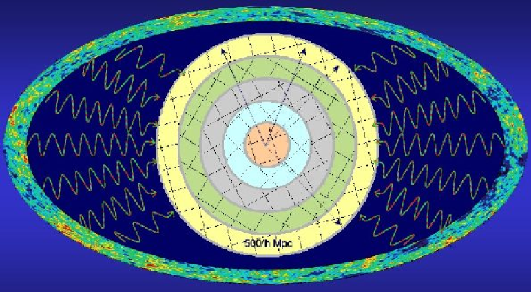
Figure 1: Sketch of the adopted stacking and randomization process. The passage of CMB photons through the dark matter distribution of the Universe is followed by stacking the gravitational potential boxes of the MS, which are $500\,h^{-1}{\rm Mpc}$ on a side (comoving). Shells of thickness $500\,h^{-1}{\rm Mpc}$ are filled with periodic replicas of the box. All boxes (squares) that fall into the same shell are randomized with the same coordinate transformation (rotation and translation), which, in turn, differs from shell to shell.

From an experimental point of view, the improved precision of the CMB observations, in particular that of the next generation experiments, may in fact require an accurate delensing methodology and a detailed lensing reconstruction. CMB experiments targeting for instance the CMB polarization, and in particular the curl component of the polarization tensor, the so called $B$-modes from cosmological gravitational waves, may greatly benefit from a precise knowledge of the lensing effects in order to separate them from the primordial cosmological signal (Seljak & Hirata, 2004). In particular, for a correct interpretation of the data from the forthcoming Planck satellite, it will be absolutely essential to understand and model the CMB lensing, as the satellite has the sensitivity and overall instrumental performance for measuring the CMB lensing with good accuracy. We note that a first detection of CMB lensing in data from the Wilkinson Microwave Anisotropy Probe (WMAP) combined with complementary data has already been claimed by (Smith et al., 2007) and (Hirata et al., 2008).

In this study we introduce a new methodology for the construction of all-sky lensing-potential and deflection-angle maps, based on a very large cosmological simulation, the Millennium run (Springel et al., 2005). As a first step in the analysis of the maps produced using the MS dark matter distribution, we have determined the interval of angular scales on which these maps match the semi-analytical expectations, since we expected a lack of lensing power on large scales, due to the finite volume of the N-body simulation. To compensate for this effect, we have implemented a method for adding large-scale power which allows to recover the correct lensing signal on the scales outside this interval, i.e. on scales larger than the MS box size. At the other extreme, at the smallest resolved scales, we are interested in the question whether our maps show evidence for extra lensing power due to the accurate representation of higher-order non-linear effects in our simulation methodology. On these small scales, the impact of non-Gaussianities from the mapping of non-linear lenses is expected to be largest.

This paper is organized as follows. In Section 2, we briefly describe the basic aspects of lensing relevant to our work. In Section 3, we describe the N-body simulation and the details of our map-making procedure. In Section 4, we present the lensing-potential and deflection-angle maps, and study the distribution of power in the angular domain. In Section 5 we provide a summary and discussion.

2 Lensed maps of the CMB via the Born approximation

In what follows we will consider the small-angle scattering limit, i.e. the case where the change in the comoving separation of CMB light-rays, owing to the deflection caused by gravitational lensing from matter inhomogeneities, is small compared to the comoving separation of the undeflected rays. In this case it is sufficient to calculate all the relevant integrated quantities, i.e. the so-called lensing-potential and its angular gradient, the deflection-angle, along the undeflected rays. This small-angle scattering limit corresponds to the so-called “Born approximation”.

We treat the CMB last scattering as an instantaneous process and neglect reionization. Adopting conformal time and comoving coordinates in a flat geometry (Ma et al., 1995), the integral for the projected lensing-potential due to scalar perturbations with no anisotropic stress reads

$$\Psi({\bf\hat{n}})\equiv-2\int_{0}^{r_{*}}\frac{r_{*}-r}{r_{*}r}\,\frac{\Phi(r{\bf\hat{n}};\eta_{0}-r)}{c^{2}}\,{\rm d}r\,,$$ (1)

while the corresponding deflection-angle integral is

$$\boldsymbol{\alpha}({\bf\hat{n}})\equiv-2\int_{0}^{r_{*}}\frac{r_{*}-r}{r_{*}r}\,\nabla_{\bf\hat{n}}\frac{\Phi(r{\bf\hat{n}};\eta_{0}-r)}{c^{2}}\,{\rm d}r\,,$$ (2)

where $r$ is the comoving distance, $r_{*}\simeq 10^{4}$ Mpc is its value at the last-scattering surface, $\eta_{0}$ is the present conformal time, $\Phi$ is the physical peculiar gravitational potential generated by density perturbations, and $[1/r]\nabla_{\hat{\bf n}}$ is the two dimensional (2D) transverse derivative with respect to the line-of-sight pointing in the direction ${\hat{\bf n}}\equiv(\vartheta,\varphi)$ (Hu, 2000; Bartelmann & Schneider, 2001; Refregier, 2003; Lewis & Challinor, 2006).

Actually, the lensing potential is formally divergent owing to the $1/r$ term near $r=0$; nonetheless, this divergence affects the lensing potential monopole only, which can be set to zero, since it does not contribute to the deflection-angle. In this way the remaining multipoles take a finite value and the lensing potential field is well defined (Lewis & Challinor, 2006). Analytically, the full information about the deflection angle is contained in the lensing potential, but numerically the two equations (1) and (2) are generally not equivalent, and it will typically be more accurate to solve the integral (2) directly to obtain the deflection angle instead of finite-differencing the lensing potential.

If the gravitational potential $\Phi$ is Gaussian, the lensing potential is Gaussian as well. However, the lensed CMB is non-Gaussian, as it is a second order cosmological effect produced by cosmological perturbations onto CMB anisotropies, yielding a finite correlation between different scales and thus non-Gaussianity. This is expected to be most important on small scales, due to the non-linearity already present in the underlying properties of lenses.

The most advanced approach developed so far for the construction of all-sky lensed CMB maps (Lewis, 2005) employs a semi-analytical modeling of the non-linear power spectrum (Smith et al., 2003), and derives from that the lensing potential and deflection angle templates assuming Gaussianity. This approach is therefore accurate for what concerns the two point correlation function of the lensing potential, as long as the non-linear two-point power of the matter is modeled correctly, but it ignores the influence of any statistics of higher order, which is expected to become relevant on small scales, where the non-linear power is most important. The use of N-body simulations to calculate the lensing has the advantage to possess a built-in capability of accurately taking into account all the effects of non-linear structure formation. On the other hand, the use of N-body simulations also faces limitations due to their limited mass and spatial resolution, and from their finite volume, as we will discuss later on in more detail.

For what concerns the line-of-sight integration in Eqs. (1) and (2), the Born-approximation along the undeflected photon path holds to good accuracy and allows to obtain results which include the non-linear physics. Even on small scales, in fact, this approximation can be exploited in the small-angle scattering limit, i.e. for typical deflections being of the order of arcminutes or less (Hirata & Seljak, 2003; Shapiro & Cooray, 2006). For example, a single cluster typically gives deflection angles of a few arcminutes, while smaller structures, such as galaxies, lead to arcsecond deflections. Furthermore, it can be shown that the Born-approximation also holds in ‘strong’ lensing cases, provided that the deflection angles are equally small. Finally, second order corrections to the Born approximation (for instance a non-vanishing curl component) are expected to be subdominant with respect to the non-linear structure evolution effects on small scales (Lewis & Challinor, 2006). For these reasons, we argue that this approximation should be accurate enough for calculating all-sky weak lensing maps of the CMB based on cosmological N-body simulations.

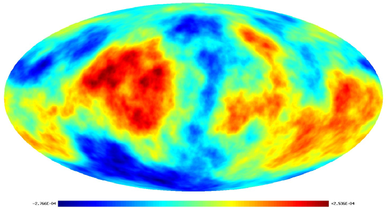
Figure 2: The simulated all-sky map of the lensing potential computed with the map-making procedure combined with the LS adding method as described in the text.

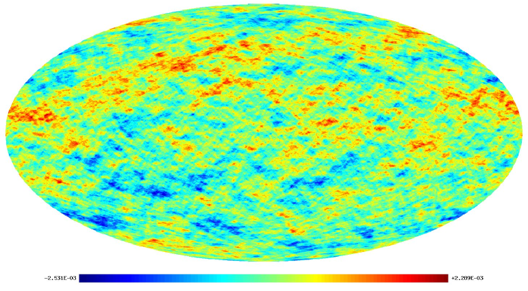
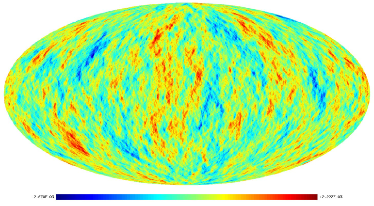
Figure 3: Simulated all-sky maps of the deflection-angle components along the $\vartheta$ direction (top panel), and along the $\varphi$ direction (bottom panel), in radians.

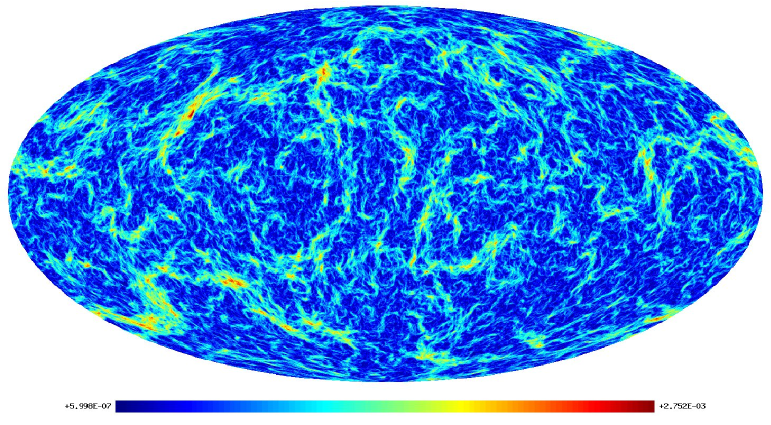
Figure 4: Top panel: Simulated all-sky map of the deflection-angle modulus (in radians), obtained with the map-making procedure combined with the LS adding method as described in the text.

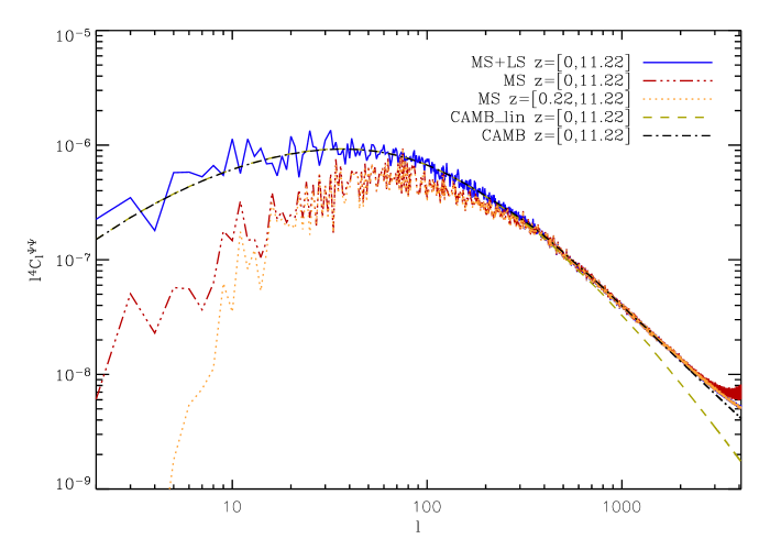
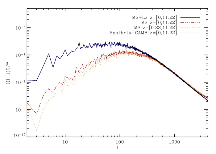
Figure 5: Top panel: The power spectrum of the simulated lensing potential map of Fig. 2 (blue solid line), compared with the power spectrum of the lensing potential obtained with the CAMB code (dashed-dotted black line), which also includes an estimate of the non-linear contributions (Smith et al., 2003). The red dashed-3dotted and orange dotted lines differ only in the starting redshift for the line-of-sight integration used in the map-making. While the result shown in red begins at $z=0$, the orange line gives the result for a start at $z=0.22$. Finally, the light-green dashed line represents the linear lensing potential power spectrum from the CAMB code. Bottom panel: The power spectrum (in radians squared) of the simulated deflection angle modulus map shown in the upper panel of Fig. 4 (blue solid line), compared with the power spectrum (dashed-dotted black line) of the synthetic deflection angle modulus map obtained as a Gaussian realization from the CAMB lensing potential power spectrum. As above, the red dashed-3dotted and orange dotted lines differ only in the starting redshift of the line-of-sight integration, as labelled. The red line is for the full redshift interval, the orange one for a start at $z=0.22$, as described in the text.

3 Map-making procedure for the Millennium Simulation

The Millennium Simulation (MS) is a high-resolution N-body simulation carried out by the Virgo Consortium (Springel et al., 2005). It uses $N=2160^{3}\simeq 1.0078\times 10^{10}$ collisionless particles, with a mass of $8.6\times 10^{8}\,h^{-1}{\rm M}_{\odot}$, to follow structure formation from redshift $z=127$ to the present, in a cubic region $500\,h^{-1}{\rm Mpc}$ on a side, and with periodic boundary conditions. Here $h$ is the Hubble constant in units of $100\,{\rm km\,s^{-1}Mpc^{-1}}$. With ten times as many particles as the previous largest computations of this kind (Colberg et al., 2000; Evrard et al., 2002; Wambsganss et al., 2004), it features a substantially improved spatial and time resolution within a large cosmological volume.

The cosmological parameters of the MS are as follows. The ratio between the total matter density and the critical one is $\Omega_{m}=0.25$, of which $\Omega_{b}=0.045$ is in baryons, while the density of cold dark matter (CDM) is given by $\Omega_{\rm CDM}=\Omega_{m}-\Omega_{b}$. The spatial curvature is assumed to be zero, with the remaining cosmological energy density made up by a cosmological constant, $\Omega_{\Lambda}=0.75$. The Hubble constant is taken to be $H_{0}=73\,{\rm km\,s^{-1}Mpc^{-1}}$. The primordial power spectrum of density fluctuations in Fourier space is assumed to be a simple scale-invariant power law of wavenumber, with spectral index $n_{s}=1$. Its normalization is set by the rms fluctuations in spheres of radius $8h^{-1}$ Mpc, $\sigma_{8}=0.9$, in the linearly extrapolated density field at the present epoch. The adopted parameter values are consistent with a combined analysis of the 2dF Galaxy Redshift Survey (2dfGRS) and the first year WMAP data (Colless et al., 2001; Spergel et al., 2003).

Thanks to its large dynamic range, the MS has been able to determine the non-linear matter power spectrum over a larger range of scales than possible in earlier works (Jenkins et al., 1998). Almost five orders of magnitude in wavenumber are covered (Springel et al., 2005). This is a very important feature for studies of CMB lensing, as we expect that this dynamic range, combined with the method for adding large-scale structures described in the next section, can be leveraged to obtain access to the full non-Gaussian statistics of the lensing signal, limited only by the the maximum angular resolution resulting from the gravitational softening length and particle number of MS. We stress again that the lensed CMB is non-Gaussian even if the underlying lenses do possess a Gaussian distribution. Moreover, the non-linear evolution of large scale structures produces a degree of non-Gaussianity in the lenses distribution which contributes to the non-Gaussian statistics of the lensed CMB on small scales. This non-Gaussian contribution can be computed only via the use of N-body simulations which are able to accurately describe the non-linear evolution of the lenses. These non-linearities are known to alter the lensed temperature power spectrum of CMB anisotropies by about $\sim 0.2\%$ at $\ell\sim 2000$ and by $\sim 1\%$ or more on smaller scales. But, much more notably, they introduce $\sim 10\%$ corrections to the B-mode polarization power on all the scales (Lewis, 2005; Lewis & Challinor, 2006).

Our map-making procedure is based on ray-tracing of the CMB photons in the Born approximation through the three-dimensional (3D) field of the peculiar gravitational potential. The latter is precomputed and stored for each of the MS output times on a Cartesian grid with a mesh of dimension $2560^{3}$ that covers the comoving simulation box of volume $(500\,h^{-1}{\rm Mpc})^{3}$. The gravitational potential itself has been calculated by first assigning the particles to the mesh with the clouds-in-cells mass assignment scheme. The resulting density field has then been Fourier transformed, multiplied with the Green’s function of the Poisson equation in Fourier space, and then transformed back to obtain the potential. Also, a slight Gaussian smoothing on a scale $r_{s}$ equal to 1.25 times the mesh size has been applied in Fourier space in order to eliminate residual anisotropies on the scale of the mesh, and a deconvolution to filter out the clouds-in-cells mass assignment kernel has been applied as well. The final potential field hence corresponds to the density field of the MS (which contains structures down to the gravitational softening length of $5\,h^{-1}{\rm kpc}$) smoothed on a scale of $\simeq 200\,h^{-1}{\rm kpc}$.

In order to produce mock maps that cover the past light-cone over the full sky, we stack the peculiar gravitational potential grids around the observer (which is located at $z=0$), producing a volume which is large enough to carry out the integration over all redshifts relevant for CMB lensing. For simplicity, we only integrate out to $z_{*}=11.22$ in this study, which corresponds to a comoving distance of approximately $r_{*}\sim 7236\,h^{-1}{\rm Mpc}$ with the present choice of cosmological parameters. Indeed, the lensing power from still higher redshifts than this epoch is negligible for CMB lensing, as we will discuss in the next section. But we note that our method could in principle be extended to still higher redshifts, up to the starting redshift $z=127$ of the simulation.

The above implies that the simulation volume needs to be repeated roughly $14.5$ times along both the positive and negative directions of the three principal Cartesian axes $x$, $y$, and $z$, with the origin at the observer. However, the spacing of the time outputs of the MS simulation is such that it corresponds to an average distance of $140\,h^{-1}{\rm Mpc}$ (comoving) on the past light-cone. We fully exploit this time resolution and use 53 outputs of the simulation along our integration paths. In practice this means that the data corresponding to a particular output time is utilized in a spherical shell of average thickness $140\,h^{-1}{\rm Mpc}$ around the observer.

The need to repeat the simulation volume due to its finite size immediately means that, without augmenting large-scale structures, the maps will suffer from a deficit of lensing power on large angular scales, due to the finite MS box size. More importantly, a scheme is required to avoid the repetition of the same structures along the line of sight. Previous studies that constructed simulated light-cone maps for small patches of the sky typically simply randomized each of the repeated boxes along the past lightcone by applying independent random translations and reflections (e.g. Springel et al., 2001). However, in the present application this procedure would produce artefacts like ripples in the simulated deflection-angle field, because the gravitational field would become discontinuous at box boundaries, leading to jumps in the deflection angle. It is therefore mandatory that the simulated lensing potential of our all sky maps is everywhere continuous on the sky, which requires that the 3D tessellation of the peculiar gravitational potential is continuous transverse to every line of sight.

Our solution is to divide up the volume out to $z_{*}$ into spherical shells, each of thickness $500\,h^{-1}{\rm Mpc}$ comoving (obviously the innermost shell is actually a sphere of comoving radius $250\,h^{-1}{\rm Mpc}$, centered at the observer). All the simulation boxes falling into the same shell are made to undergo the same, coherent randomization process, i.e. they are all translated and rotated with the same random vectors generating a homogeneous coordinate transformation throughout the shell. But this randomization changes from shell to shell. Figure 1 shows a schematic sketch of this stacking process. For simplicity, the diagram does not illustrate the additional shell structure stemming from the different output times of the simulation. As discussed before, this simply means that the underlying potential grid is updated on average  3-4 times with a different simulation output when integrating through one of the rotated and translated $500\,h^{-1}{\rm Mpc}$ shells, but without changing the coordinate transformation. Notice that our stacking procedure eliminates any preferred direction in the simulated all-sky maps.

In order to define the gravitational potential at each point along a ray in direction $\hat{\bf n}$, we employ spatial tri-linear interpolation in the gravitational potential grid. It is then easy to numerically calculate the integral potential for each ray, based for example on a simple trapezoidal formula, which we use in this study. Obtaining the deflection angle could in principle be done by finite differencing a calculated lensing potential map, either in real space or the harmonic domain. However, the accuracy of this approach would depend critically on the angular resolution of the map. Also, the sampling of the gravitational potential in the direction transverse to the line-of-sight varies greatly with the distance from the observer, so in order to extract the maximum information from the simulation data down to the smallest resolved scales in the potential field, we prefer to directly integrate up the deflection angle vector along each light ray in our map. For this purpose we first use a fourth-order finite-differencing scheme to compute the local 3D grid of the gradient of the gravitational potential, which is then again tri-linearly interpolated to each integration point along a line-of-sight. In this way, we calculate the deflection angle directly via equation (2) along the paths of undeflected light rays.

Finally, we need to select a pixelization of the sky with a set of directions ${\bf\hat{n}}\equiv(\vartheta,\varphi)$. We here follow the standard approach introduced by the HEALPix hierarchical tessellation of the unit sphere (Gorski et al., 2005).

4 Simulated maps of the lensing potential and deflection angle

In Figs. 2, 3, and 4, we show full-sky maps of the lensing potential, the deflection angle $\vartheta$/$\varphi$-components, and the deflection angle modulus $|\boldsymbol{\alpha}|$, respectively, obtained with the map-making technique described in the previous section combined with a semi-analytic procedure (to be explained below) augmenting the lensing power on scales beyond the MS box size. These maps are generated with a HEALPix pixelization parameter $N_{\rm side}=2048$, and have an angular resolution of $\sim 1.72^{\prime}$ (Gorski et al., 2005), with 50331648 pixels in total.

Several interesting features should be noted in these maps. The distribution of the lensing potential, where the monopole and dipole have been cut to simplify the visual inspection, appears to be dominated by large features, which are probably simply arising from the projection of the largest scale gravitational potential fluctuations along the line-of-sight. However, the strength of local lensing distortions in the CMB cannot be directly inferred from the map of the lensing potential, as for the lensing deflection only the gradient of the potential is what really matters.

The maps showing the lensing deflection angle components have interesting features as well. First of all, the signal in the two components of the deflection angle appears to possess two morphologically distinct regimes, characterized on one hand by a diffuse background distribution, caused probably by the lines-of-sight where no dominant structures are encountered, and on the other hand by sharp features, caused probably by massive CDM structures which give rise to the largest deflections in the line-of-sight integration itself. The same features are evident in the map of the modulus of the deflection-angle.

The mean value of $|\boldsymbol{\alpha}|$ in our simulated maps is $2.36^{\prime}$, while its standard deviation is $1.25^{\prime}$. The latter has to be compared with the corresponding value obtained via the angular differentiation of synthetic Gaussian maps produced with the lensing potential power spectrum generated by the publicly available Code for Anisotropies in the Microwave Background (CAMB) using the MS cosmological parameters, as we explain in detail below. We find only a $0.03\%$ difference for the rms of the $|\boldsymbol{\alpha}|$-maps from MS and CAMB, when using the same maximum redshift of line-of-sight integration, i.e. $z_{\textrm{max}}=11.22$. On the other hand, if we set $z_{\textrm{max}}=1100$ in CAMB, we find that our estimate is $\sim 1.7\%$ smaller than the semi-analytic one, due to the missed contribution from sources beyond $z\sim 11$ in our map-making procedure. For comparison, we also evaluate semi-analytically the expected change in the standard deviation of $|\boldsymbol{\alpha}|$ when inserting in CAMB more recent estimates of the cosmological parameters (Komatsu et al., 2008). In this case the rms from MS is $\sim 6\%$ and $\sim 4.2\%$ greater than the semi-analytical prediction when in CAMB we set $z_{\textrm{max}}=11.22$ and $z_{\textrm{max}}=1100$, respectively.

The lensing potential and deflection angle maps of Figs. 2 and 4 have been obtained combining the map-making procedure described in the previous section with the method for adding large-scale power that we now explain.
Firstly, we have measured the power spectra of the simulated maps obtained from the MS scales only, i.e., using the routine ANAFAST of the HEALPix package, we have independently measured the power spectra of the lensing potential ($C_{l}^{\Psi\Psi}$) and deflection angle modulus ($C_{l}^{\alpha\alpha}$) of the MS simulated maps, without exploiting the relations between the lensing potential and the $\pm 1$-spin components of the deflection angle, which hold in the spherical harmonic domain (Hu, 2000). Secondly, using the MS cosmological parameters, we have evaluated the semi-analytical power spectrum of the lensing potential from CAMB, including the estimate of the contribution from non-linearity (Smith et al., 2003) and stopping the line-of-sight integration redshift up to $z=11.22$. Using the lensing potential power spectrum from CAMB, we have then produced the corresponding synthetic map (and its angular differentiation) obtained as a Gaussian realization generated with the HEALPix code SYNFAST, in order to produce the synthetic map of the deflection angle modulus from the semi-analytic expectations of CAMB. From this map we have then extracted the power spectrum of the deflection angle modulus, and after deconvolution from the HEALPix pixel window function, we have compared it, together with the lensing potential power spectrum, to the corresponding deconvolved MS power spectra.

The top panel of Fig. 5 shows the primary result of this comparison. The black dashed-dotted line represents the semi-analytic prediction of the lensing potential angular power spectrum obtained from CAMB as discussed above. This has been compared with the red dashed-3dotted line obtained with the map-making procedure previously described, and which represents the result for the full integration starting at $z=0$ and ending at $z=11.22$. In this case, a power deficiency on large scales with respect to the semi-analytical prediction is evident, and confined to a multipole range corresponding to one degree or more in the sky. The same for the orange dotted line which gives the MS lensing potential power spectrum obtained from a line-of-sight integration starting at a redshift of $z=0.22$ and ending at $z=11.22$; comparing the two curves, a power decrease at low $\ell$ is easily observable in the orange dotted line, with respect to the red dashed-3dotted one, illustrating the influence of the lack of comoving scales greater than $500\,h^{-1}{\rm Mpc}$ in the MS. As expected, this effect is evident in the multipole range corresponding to a few degrees or more, which is about the size of the MS box at the redshift most relevant for CMB lensing, i.e. $z\simeq 1$. However, towards larger $\ell$, the deficit of large-scale power quickly decreases, and becomes negligible at scales $l\mathrel{\hbox to0.0pt{\lower 3.0pt\hbox{$\sim$}\hss}\raise 2.0pt\hbox{$>$}}350$. Between these scales and $l\sim 2500$, there is quite good agreement between the MS lensing power spectrum and the semi-analytic prediction, but at $2500\lesssim l\lesssim 4000$ the full MS signal for the lensing potential actually slightly exceeds the semi-analytic result. On this multipole range, the red dashed line is dominated by Poisson noise, but the slight excess of power is clearly observable from the orange dot line, in which there is no contribution from the low redshift integration at $z\lesssim 0.2$. We ascribe this power excess to the matter non-linearities accurately reproduced from the Millennium Simulation. Finally, at $l\sim 4000$ the MS signal is dominated by Poisson sampling noise from low-redshift potential integration. In fact, at very low redshifts, the $1.72^{\prime}$ angular resolution of our map is comparable and even smaller than the intrinsic angular resolution corresponding to the spatial grid of the 3D gravitational potential field we use. This is evident in Fig. 6, where we compare the map angular resolution of $1.72^{\prime}$ (red dashed line) with the effective angular resolution corresponding to the intrinsic grid spacing ($195\,h^{-1}{\rm kpc}$) of the 3D gravitational potential field as function of redshift. Because the line-of-sight integral for the projected lensing potential involves a $1/r$ weighting term, the resulting noise terms are unfavourably amplified when the lensing potential is considered.

The comparison above has been used to evaluate the multipole range, $0\lesssim l\lesssim 350$, not covered by the MS scales. On this interval we have applied the LS adding method: from the CAMB and MS maps of the lensing potential, we have extracted the two corresponding ensembles $\Psi_{lm}^{CAMB}$ and $\Psi_{lm}^{MS}$ of spherical harmonic coefficients, respectively. Since on low multipoles the effects of the non-Gaussianity from the non-linear scales are negligible and the $\Psi_{lm}$ are independent, we have generated a joined ensemble of $\tilde{\Psi}_{lm}$, where $\tilde{\Psi}_{lm}=\Psi_{lm}^{CAMB}$ for $0\leq l\leq 350$ and $\tilde{\Psi}_{lm}=\Psi_{lm}^{MS}$ for $l>350$. Finally, we have generated the synthetic maps of the lensing potential and deflection angle as non-Gaussian constrained realizations, inserting the $\tilde{\Psi}_{lm}$ as input in SYNFAST, as shown in Figs. 2-4.

These maps have the peculiarity of reproducing the non-linear and non-Gaussian effects of the MS non-linear dark matter distribution at multipoles $l>350$, while at the same time including the contribution from the large scales at $l\leq 350$, where the lensing potential follows mostly the linear trend as shown from the light-green dot-dashed line in Fig. 5. The blue solid curve in the same Figure represents the resulting power spectrum of the lensing potential map after the LS addition.

The bottom panel of Fig. 5, shows the corresponding power spectra for the physically and numerically more meaningful deflection angle. Here we show a comparison of the power spectrum of the deflection angle modulus ($C_{l}^{\alpha\alpha}$) measured for the MS simulated maps, in the absence of LS supplying, with the semi-analytic prediction constructed with CAMB and SYNFAST, as explained above. Again, we find a deficit of power on large scales, and a reassuring agreement over about one order of magnitude in $l$ on intermediate scales. However, a slight excess of power over the semi-analytic predictions is easily seen at $l\mathrel{\hbox to0.0pt{\lower 3.0pt\hbox{$\sim$}\hss}\raise 2.0pt\hbox{$>$}}2500$. As previously mentioned, it can be attributed to the non-linear evolution of the MS structures. Finally, the blue solid line represents the power spectrum extracted from the deflection angle modulus map of Fig. 4, after adding large-scale structures.

Our map making procedure offers very good resolution at the most important redshift for lensing of the CMB, $z\sim 1$ (see also Fig. 7), where the intrinsic angular resolution of our potential grid is six times better than the angular resolution of the full-sky map. We therefore think that this higher small-scale power is a direct result of the more accurate representation of non-linear structure formation in our map simulation methodology. In fact, in our current maps we are still far from probing the most non-linear scales accessible in principle with our simulation. Those are a factor 40 smaller (namely $5\,h^{-1}{\rm kpc}$) than resolved by the potential grid we have employed. However, using such a fine mesh is currently impractical, and would lead to angular resolutions in full-sky maps that are unaccessible even by the Planck satellite. However, for a smaller solid-angle of the map, these scales can be probed with a different ray-tracing technique (Hilbert et al., 2007).

We note that the semi-analytic prediction for the power spectrum of the deflection angle modulus has been evaluated as an angular gradient in the harmonic domain of a synthetic lensing potential Gaussian map; that is accurate since in this approach we work with Fourier modes right from the start anyway. From a numerical point of view, the integral and derivative operators in Eq. (2) do however not commute, even if they analytically do, in the sense that finite differencing our measured projected potential will not necessarily give the same result as numerically integrating the deflection angle along each line of sight. The latter approach is more accurate, expecially at very high resolution, and it has been used by us in the comparison above since numerically integrating the deflection angle along each line of sight allows to preserve the contribution from the non-linear scales in a more efficient way than simply operating in the harmonic domain.

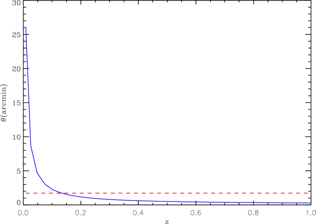
Figure 6: Comparison between the angular resolution of $1.72^{\prime}$ of our full-sky maps (red dashed line) and the redshift-dependent, effective angular resolution (blue solid line) corresponding to the intrinsic grid spacing ($\sim 200\,h^{-1}{\rm kpc}$) of the three-dimension gravitational potential field constructed from the Millennium Simulation.

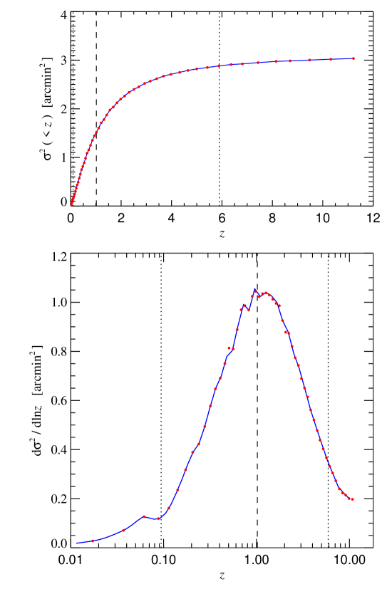
Figure 7: The cumulative and differential variance of the deflection angle map as a function of redshift. The symbols mark the different output times of the Millennium Simulation. The vertical dashed line gives the redshift that corresponds to the 50% quartile of the total variance in our maps, which is approximately at $z\sim 1$. The dotted lines mark the 5% and 95% percentiles, indicating that 90% of our signal in the deflection angle power spectrum is produced in the redshift range $z\sim 0.1$ to $z\sim 6.0$. Note however that we have lost a few percent of the total power due to our truncation of the integration at $z=11.22$. When included, this would slightly shift these precentiles to higher redshift.

Finally, we consider the distribution of the deflection angle power along the line-of-sight. In Fig. 7, we show the cumulative and differential variance of the deflection angle as a function of redshift. We see that the most important contributions to the final signal stem from $z\sim 1$, i.e. about half ways between the last scattering surface and the observer, as expected. This also allows us to assess the relative error introduced by stopping the integration at $z\simeq 11$, which is of the order of a few percent, as mentioned above.

5 Conclusions

We constructed the first all sky maps of the cosmic microwave background (CMB) weak-lensing potential and deflection angle based on a high-resolution cosmological N-body simulation, the Millennium Run Simulation (MS). The lensing potential and deflection angle are evaluated in the Born approximation by directly ray-tracing through a three-dimensional, high-resolution mesh of the evolving peculiar gravitational potential and its gradient. The time evolution is approximated by 53 simulation outputs between redshift $z=0$ and $z\simeq 11$, each used to cover a thin redshift interval corresponding to a shell in the past light-cone around the observer. To prevent artificial repetition of structures along the line-of-sight, while at the same time avoiding discontinuities in the force transverse to a line-of-sight, we tessellate shells of comoving thickness corresponding to the size of the box ($500\,h^{-1}{\rm Mpc}$) with periodic replicas which are coherently rotated and translated within each shell by a random amount. Moreover, in order to include the contribution to the lensing signal from the scales larger than the MS box size, we have implemented a method for adding large-scale structure as described in the text.

Using the Hierarchical Equal Area Latitude Pixelization (HEALPIX) package for obtaining a uniform sky-coverage, we have constructed simulated CMB lensing maps with $\sim 5$ million pixels and an angular resolution of $\sim 1.72^{\prime}$, based on potential fields calculated on $2560^{3}$ meshes from the Millennium simulation. In the present study, we analyze the power spectrum of the lensing potential and the deflection angle, and compare it with predictions made by semi-analytic approaches. We note that our general approach for map-making can be extended to other CMB foregrounds, including the Integrated Sachs-Wolfe (ISW) and Rees-Sciama effects at low redshifts, as well as estimates of the Sunyaev Zel’dovich (SZ) effects, or of the X-ray background. This will in particular allow studies of the cross-correlation of the lensing of CMB temperature and polarization with these effects, which will be the subject of a forthcoming study. In our approach we do not take into account the contributions of the baryonic physics to the lensing effects on the CMB. We expect in fact that these contributions could be non-negligible only on the typical scales of cluster cores and below, thus well above $l\sim 3000$. Our comparison of the angular power spectrum of the lensing-potential and the deflection-angle with semi-analytic expectations reveals two different regimes in our results. First, for multipoles up to $l\sim 2500$, our simulated maps produce a lensing signal that matches the semi-analytic expectation. Second, we find evidence for a slight excess of power in our simulated maps on scales corresponding to few arcminutes and less, which we attribute to the accurate inclusion of non-linear power in the Millennium simulation. It will be especially interesting to study the non-Gaussianities in the signal we found and its implied consequences for CMB observations.

The new method proposed here demonstrates that an all-sky mapping of CMB lensing can be obtained based on modern high-resolution N-body simulations. This opens the way towards a full and accurate characterization of CMB lensing statistics, which is unaccessible beyond the power spectrum with the existing semi-analytical techniques. This is relevant in view of the forthcoming CMB probes, both as a way to detect, extract and study the CMB lensing signal, which carries hints on the early structure formation as well as the onset of cosmic acceleration, and as a tool to distinguish CMB lensing from the Gaussian contribution due to primordial gravitational fluctuations.

References

- Acquaviva & Baccigalupi (2006) Acquaviva V., Baccigalupi C., 2006, Phys. Rev. D 74, 103510.
- Amblard et al. (2004) Amblard A., Vale C., White M., 2004, New Astron. 9, 687.
- Bartelmann & Schneider (2001) Bartelmann M., Schneider P., 2001, Phys. Rept. 340, 291.
- Colberg et al. (2000) Colberg J.M. et al., 2000, Mon. Not. R. Astron. Soc. 319, 209.
- Colless et al. (2001) Colless M. et al., 2001, Mon. Not. R. Astron. Soc. 328, 1039.
- Evrard et al. (2002) Evrard A.E. et al., 2002, Astrophys. J. 573, 7.
- Geller & Hucra (1989) Geller M.J., Huchra J.P., 1989, Science 246, 897.
- Gorski et al. (2005) Gorski K.M., 2005, Astrophys. J. 622, 759.
- Gott et al. (2005) Gott J.R.I. et al., 2005, Astrophys. J. 624, 463.
- Hilbert et al. (2007) Hilbert S., White S.D.M., Hartlap J., Schneider P., 2007, Mon. Not. R. Astron. Soc. , in press.
- Hirata et al. (2008) Hirata C.M., Ho S., Padmanabhan N., Seljak U., Bahcall N., arXiv:0801.0644v2.
- Hirata & Seljak (2003) Hirata C.M., Seljak U., 2003, Phys. Rev. D 68, 083002.
- Hu (2000) Hu W., 2000, Phys. Rev. D 62, 043007-1.
- Hu et al. (2006) Hu W., Huterer D., Smith K.M., 2006, Astrophys. J. Lett. 650, L13.
- Jenkins et al. (1998) Jenkins A. et al., 1998, Astrophys. J. 499, 20.
- Komatsu et al. (2008) Komatsu E. et al., 2008, arXiv:0803.0547v1.
- Lewis (2005) Lewis A., 2005, Phys. Rev. D 71, 083008.
- Lewis & Challinor (2006) Lewis A., Challinor A., 2006, Phys. Rept. 429, 1.
- Ma et al. (1995) Ma C.P., Bertschinger E., 1995, Astrophys. J. 455, 7.
- Refregier (2003) Refregier A., 2003, Annu. Rev. Astron. Astrophys. 41, 645.
- Seljak & Hirata (2004) Seljak U., Hirata C.M., 2004, Phys. Rev. D 69, 043005.
- Shapiro & Cooray (2006) Shapiro C., Cooray A., 2006, JCAP 0603, 007.
- Smith et al. (2003) Smith R.E. et al., The Virgo Consortium, 2003, Mon. Not. R. Astron. Soc. 341, 1311.
- Smith et al. (2007) Smith K.M., Zahn O., Dore O., 2007, Phys. Rev. D 76, 043510.
- Spergel et al. (2003) Spergel D.N. et al.(2003), Astrophys. J. Suppl. 148, 175.
- Springel et al. (2001) Springel V., Frenk C.S., White S.D.M., 2006, Nature 1137, 440.
- Springel et al. (2005) Springel V., White M., Hernquist L., 2001, Astrophys. J. 549, 681.
- Wambsganss et al. (2004) Wambsganss J., Bode P., Ostriker J.P., 2004, Astrophys. J. Lett. 606, L93.