Multiuser MIMO Achievable Rates with Downlink Training and Channel State Feedback

Abstract

We consider a MIMO fading broadcast channel and compute achievable ergodic rates when channel state information is acquired at the receivers via downlink training and it is provided to the transmitter by channel state feedback. Unquantized (analog) and quantized (digital) channel state feedback schemes are analyzed and compared under various assumptions. Digital feedback is shown to be potentially superior when the feedback channel uses per channel state coefficient is larger than 1. Also, we show that by proper design of the digital feedback link, errors in the feedback have a minor effect even if simple uncoded modulation is used on the feedback channel. We discuss first the case of an unfaded AWGN feedback channel with orthogonal access and then the case of fading MIMO multi-access (MIMO-MAC). We show that by exploiting the MIMO-MAC nature of the uplink channel, a much better scaling of the feedback channel resource with the number of base station antennas can be achieved. Finally, for the case of delayed feedback, we show that in the realistic case where the fading process has (normalized) maximum Doppler frequency shift $0\leq F<1/2$, a fraction $1-2F$ of the optimal multiplexing gain is achievable. The general conclusion of this work is that very significant downlink throughput is achievable with simple and efficient channel state feedback, provided that the feedback link is properly designed.

I Introduction

In the downlink of a cellular-like system, a base station equipped with multiple antennas communicates with a number of terminals, each possibly equipped with multiple receive antennas. If a traditional orthogonalization technique such as TDMA is used, the base station transmits to a single receiver on each time-frequency resource and thus is limited to point-to-point MIMO techniques [1, 2]. Alternatively, the base station can use multi-user MIMO to simultaneously transmit to multiple receivers on the same time-frequency resource. Under the assumption of perfect channel state information at the transmitter (CSIT) and at the receivers (CSIR), a combination of single-user Gaussian codes, linear beamforming and “Dirty-Paper Coding” (DPC) [3] is known to achieve the capacity of the MIMO downlink channel [4, 5, 6, 7, 8]. When the number of base station antennas is larger than the number of antennas at each terminal, the capacity of the MIMO downlink channel is significantly larger than the rates achievable with point-to-point MIMO techniques [4, 9, 10].

Given the widespread applicability of the MIMO downlink channel model (e.g., to cellular, WiFi, and DSL), it is of great interest to design systems that can operate near the capacity limit. Although realizing the optimal DPC coding strategy still remains a formidable challenge (see for example [11, 12, 13]), it has been shown that linear beamforming without DPC performs quite close to capacity when combined with user selection, again under the simplifying assumption of perfect channel state information (see for example [14, 15]).

In real systems, however, channel state information is not a priori provided and must be acquired, e.g., through training. Acquiring the channel state is a challenging and resource-consuming task in time-varying systems, and the obtained information is inevitably imperfect. It is therefore critical to understand what rates are achievable under realistic channel state information assumptions, and in particular to understand the sensitivity of achievable rates to such imperfections. To emphasize the importance of channel state information, note that in the extreme case of no CSIT at the BS and identical fading statistics (and perfect CSIR) at all terminals, the multi-user MIMO benefit is completely lost and point-to-point MIMO becomes optimal [4].

I-A Contributions of this work

The focus of this paper is a rigorous information theoretic characterization of the ergodic achievable rates of a fading multiuser MIMO downlink channel in which the UTs and the BS obtain imperfect CSIR/CSIT via downlink training and channel state feedback. Converse results on the capacity region of the MIMO broadcast channel with imperfect channel knowledge are essentially open (see for example [16] and [17] for some partial results). Here, we focus on the achievable rates of a specific signaling strategy, zero-forcing (ZF) linear beamforming. Consistently with contemporary wireless system technology, we assume that each UT estimates its own channel during a downlink training phase and then feeds back its estimate over the reverse uplink channel to the BS. The BS designs beamforming vectors on the basis of the received channel feedback, after which an additional round of downlink training is performed (essentially to inform the UTs of the selected beamformers). Our results tightly bound the rate that is achievable after this process in terms of the resources (i.e., channel symbols) used for training and feedback and the channel feedback technique.

The analysis of this paper inscribes itself in the line of works dealing with “training capacity” [18] of block-fading channels. Several previous and concurrent works have treated training and channel feedback for point-to-pont MIMO systems (see for example [19, 20, 21, 22, 23, 24, 25]) and, more recently, for MIMO broadcast channels (see for example [26, 27, 28, 29, 30, 31, 32]). However, this paper presents a number of novelties relative to prior/concurrent work:

• Rather than assuming perfect CSIR at the UT’s, we consider the realistic scenario where the UTs have imperfect CSIR obtained via downlink training. Because the imperfect CSIR is the basis for the channel feedback from the UTs, this degrades the quality of the CSIT provided to the BS in a non-negligible manner.

• Instead of idealizing the feedback channel as a fixed-rate, error-free bit-pipe, we explicitly consider transmission from each UT to the BS over the noisy feedback channel. This reveals the fundamental joint source-channel coding nature of channel feedback. In addition, this allows us to meaningfully measure the uplink resources dedicated to channel feedback and also allows for a comparison between analog (unquantized) and digital (quantized) feedback. We begin by modeling the feedback channel as an AWGN channel (orthogonal across UTs), and later generalize to a multiple-antenna uplink channel that is shared by the UTs. In this way, we precisely quantify the fundamental advantage of using the multiple BS antennas for efficient channel state feedback.

• A fundamental property of the system is that UTs are unaware of the chosen beamforming vectors, because the beamformers depend on all channels whereas each UT only has an estimate of its own channel. Several previous works (e.g., [26, 33, 34]) have resolved this uncertainty by making the unstated assumption that each UT has perfect knowledge of the post-beamforming SINR. In contrast, we make no such assumption and rigorously show that this ambiguity can be resolved by an additional round of (dedicated) training.

• Most prior work has used a worst-case uncorrelated noise argument [35][36][18] to show that imperfect CSI, at worse, leads to the introduction of additional Gaussian noise and thus the achievable rate is lower bounded by the mutual information with ideal channel state information and reduced SNR. In our case, however, this same argument yields a largely uncomputable quantity and a further step must be taken that yields a tractable lower bound in terms of the rate difference between the ideal and actual cases, rather than in terms of a SNR penalty.

• We consider delayed feedback and quantify in a simple and appealing form the loss of degrees of freedom (pre-log factor in the achievable rate) in terms of the fading channel Doppler bandwidth, which is ultimately related to UT velocity.

The analysis presented in this paper is relevant from at least two related but different viewpoints. On one hand, it provides accurate bounds on the achievable ergodic rates of the linear zero-forcing beamforming scheme with realistic channel estimation and feedback. These bounds are useful at any operating SNR (not necessarily large), and in subsequent work have been used to optimize the system resources allocated for training and feedback [37][38]. On the other hand, it yields sufficient conditions on the training and feedback such that the system achieves the same multiplexing gain (also referred to as “pre-log factor”, or “degrees of freedom”) of the optimal DPC-based scheme under perfect CSIR/CSIT. Perhaps the most striking fact about this second aspect is that the full multiplexing gain of the ideal MIMO broadcast channel can be achieved with simple pilot-based channel estimation and feedback schemes that consume a relatively small fraction of the system capacity. Indeed, a fundamental property of the MIMO broadcast channel is that the quality of the CSIT must increase with signal-to-noise ratio (SNR), regardless of what coding strategy is used, in order for the full multiplexing gain to be achievable [16, 17]. Under the reasonable assumption that the uplink channel quality is in some sense proportional to the downlink channel, our work shows that this requirement can be met using a fixed number of downlink and uplink channel symbols (i.e., system resources used for training and feedback need not increase with SNR).

When there is a significant delay in the feedback loop, the simple scheme analyzed in this paper does not attain full multiplexing gain. However, for fading processes with normalized Doppler bandwidth $F$ strictly less than $1/2$, we show the achievability of a multiplexing gain equal to $M(1-2F)$, where $M$ is the number of BS antennas. This result follows from a fundamental property of the noisy prediction error of the channel process and is closed related to Lapidoth’s high-SNR capacity of single-user fading channels without the perfect CSIR assumption [39].

The paper is organized as follows. Section II introduces the system model, describes linear beamforming, and defines the baseline estimation, feedback, and beamforming strategy. Section III develops bounds on the ergodic rates achievable by the baseline scheme. In Section IV we consider an AWGN feedback channel and particularize the rate bounds to analog and digital feedback (incorporating the effect of decoding errors for digital feedback), and compare the different feedback options. Section V generalizes the results to the setting where the feedback link is a fading MIMO multiple access channel (MAC). Section VI considers time-correlated fading and the effect of delay in the feedback link. Some concluding remarks are provided in Section VII.

II System Model

We consider a multi-input multi-output (MIMO) Gaussian broadcast channel modeling the downlink of a system where a Base Station (BS) has $M$ antennas and $K$ User Terminals (UTs) have one antenna each. A channel use of such channel is described by

$$y_{k}={\bf h}_{k}^{\sf H}{\bf x}+z_{k},\;\;k=1,\ldots,K$$ (1)

where $y_{k}$ is the channel output at UT $k$, $z_{k}\sim{\cal C}{\cal N}(0,N_{0})$ is the corresponding Additive White Gaussian Noise (AWGN), ${\bf h}_{k}\in\mbox{\bb C}^{M}$ is the vector of channel coefficients from the $k$-th UT antenna to the BS antenna array (the superscript ${\sf H}$ refers to the Hermitian, or conjugate transpose) and ${\bf x}$ is the vector of channel input symbols transmitted by the BS. The channel input is subject to the average power constraint $\mbox{\bb E}[|{\bf x}|^{2}]\leq P$.

We assume that the channel state, given by the collection of all channel vectors ${\bf H}=[{\bf h}_{1},\ldots,{\bf h}_{K}]\in\mbox{\bb C}^{M\times K}$, varies in time according to a block-fading model [40], where ${\bf H}$ is constant over each frame of length $T$ channel uses, and evolves from frame to frame according to an ergodic stationary spatially white jointly Gaussian process, where the entries of ${\bf H}$ are Gaussian i.i.d. with elements $\sim{\cal C}{\cal N}(0,1)$. Our bounds on the ergodic achievable rate do not directly depend on the frame size $T$; rather, these bounds depend only on whether the training, feedback, and data phases all occur within a frame or in different frames. In Sections IV - V we consider the simplified scenario where the three phases all occur within a single frame (i.e., the channel is constant across the phases) and fading is independent across blocks, but we remove these simplifications in Section VI. It should also be noticed that the rate lower bounds given in the following should be multiplied by the factor $(1-\Delta/T)$, where $\Delta$ denotes the total number of channel uses per frame dedicated to training and feedback. This factor is neglected in this paper since it is common to all rate bounds and since $\Delta\ll T$ in a typical slowly-fading system scenario. However, in the general case where $\Delta$ is not necessarily small with respect to $T$, the amount of training and feedback should be optimized by taking this multiplicative factor into account. Based on the bounds developed in the present paper, this system optimization is carried out in the follow-up works [37, 38].

II-A Linear beamforming

Because of simplicity and robustness to non-perfect CSIT, simple linear precoding schemes with standard Gaussian coding have been extensively considered: the transmit signal is formed as ${\bf x}={\bf V}{\bf u}$, such that ${\bf V}\in\mbox{\bb C}^{M\times K}$ is a linear beamforming matrix and ${\bf u}\in\mbox{\bb C}^{K}$ contains the symbols from $K$ independently generated Gaussian codewords. In particular, for $K\leq M$ Zero-Forcing beamforming chooses the $k$-th column ${\bf v}_{k}$ of ${\bf V}$ to be a unit vector orthogonal to the subspace ${\cal S}_{k}={\rm span}\{{\bf h}_{j}:j\neq k\}$.

We focus on the achievable ergodic rates under ZF linear beamforming and Gaussian coding. In this case, the achievable rate-sum is given by

$$\max_{\sum_{k}\mbox{\bbsmall E}[{\cal P}_{k}({\bf H})]\leq P}\;\sum_{k=1}^{K}\mbox{\bb E}\left[\log\left(1+\frac{|{\bf h}_{k}^{\sf H}{\bf v}_{k}|^{2}{\cal P}_{k}({\bf H})}{N_{0}}\right)\right].$$ (2)

where the optimal power allocation is obtained by waterfilling over the set of channel gains $\{|{\bf h}_{k}{\bf v}_{k}|^{2}:k=1,\ldots,K\}$. Performance can further be improved by using a user scheduling algorithm to select in each frame an active user subset not larger than $M$ (if $K>M$, such selection must be performed if ZF is used). Schemes for user scheduling have been extensively discussed, for example in [41, 32, 15, 42].

We focus, however, on the case $K=M$ with uniform power allocation (across users and frames: ${\cal P}_{k}({\bf H})=\frac{P}{M}$) and without user selection, in which case the per-user ergodic rate is

$$R_{k}^{\rm ZF}(P)=\mbox{\bb E}\left[\log\left(1+\frac{|{\bf h}_{k}^{\sf H}{\bf v}_{k}|^{2}P}{N_{0}M}\right)\right].$$ (3)

Because ${\bf h}_{k}$ is spatially white and ${\bf v}_{k}$ is selected independent of ${\bf h}_{k}$ (by the ZF procedure), it follows that ${\bf h}_{k}^{\sf H}{\bf v}_{k}$ is $\sim{\cal C}{\cal N}(0,1)$. As a result, $R_{k}^{\rm ZF}$ is the ergodic capacity of a point-to-point channel in Rayleigh fading with average SNR $\frac{P}{N_{0}M}$, and thus can be written in closed form as [43] $R_{k}^{\rm ZF}=\exp\left(\frac{N_{0}M}{P}\right){\rm E}_{i}\left(1,\frac{N_{0}M}{P}\right)$ where ${\rm E_{i}}(n,x)=\int_{1}^{\infty}\frac{e^{-xt}}{t^{n}}dt,\;x>0$ [44]. In the remainder of the paper $R_{k}^{\rm ZF}$ serves as a benchmark aginst which we compare the achievable rates with imperfect CSI.

This restriction is dictated by a few reasons. On one hand, the case $K=M$ without selection makes closed-form analysis (in the presence of imperfect CSI) possible. In addition, the maximum multiplexing gain is $M$ for all $K\geq M$ and hence the case $K=M$ suffices to capture the fundamental aspects of the problem (particularly at high SNR). Finally, recent results [33, 45] show that the dependence on CSI quality is roughly the same even when user selection is performed.

II-B Channel state estimation and feedback

We assume that each UT estimates its channel vector from downlink training symbols and then feeds this information back to the BS. This scenario, referred to as “closed-loop” CSIT estimation, is relevant for Frequency-Division Duplexed (FDD) systems. Our baseline system is depicted in Fig. 1 and consists of the following phases:

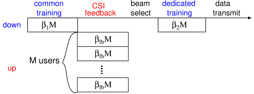
Figure 1: Channel estimation and feedback model

1. Common Training:  The BS transmits $\beta_{1}M$ shared pilots ($\beta_{1}\geq 1$ symbols per antenna) on the downlink. Each UT $k$ estimates its channel from the observation

   $${\bf s}_{k}=\sqrt{\beta_{1}P}\ {\bf h}_{k}+{\bf z}_{k}$$ (4)

   corresponding to the common training (downlink) channel output, where ${\bf z}_{k}\sim{\cal C}{\cal N}(0,N_{0}{\bf I})$. The MMSE estimate $\widetilde{{\bf h}}_{k}$ of ${\bf h}_{k}$ given the observation ${\bf s}_{k}$ is given by [46]:

   $$\widetilde{{\bf h}}_{k}=\mbox{\bb E}[{\bf h}_{k}{\bf s}_{k}^{\sf H}]\mbox{\bb E}[{\bf s}_{k}{\bf s}_{k}^{\sf H}]^{-1}{\bf s}_{k}=\frac{\sqrt{\beta_{1}P}}{N_{0}+\beta_{1}P}{\bf s}_{k}$$ (5)

   The channel ${\bf h}_{k}$ can be written in terms of the estimate $\widetilde{{\bf h}}_{k}$ and estimation noise ${\bf n}_{k}$ as:

   $${\bf h}_{k}=\widetilde{{\bf h}}_{k}+{\bf n}_{k},$$ (6)

   where ${\bf n}_{k}$ is independent of the estimate and is Gaussian with covariance $\sigma_{1}^{2}{\bf I}$ with

   $$\sigma_{1}^{2} = \frac{1}{1+\beta_{1}P/N_{0}}$$ (7)

2. Channel State Feedback:   Each UT feeds back its channel estimate $\widetilde{{\bf h}}_{k}$ to the BS immediately after completion of the common training phase. We use $\widehat{{\bf H}}=[\widehat{{\bf h}}_{1},\ldots,\widehat{{\bf h}}_{K}]\in\mbox{\bb C}^{M\times K}$ to denote the (imperfect) CSIT available at the BS; the feedback is thus a mapping, possibly probabilistic, from $\widetilde{{\bf h}}_{k}$ to $\widehat{{\bf h}}_{k}$. For now we leave the feedback scheme unspecified to allow development of general achievability bounds in Section III, and particularize to specific feedback schemes from Section IV onwards.

   In Section IV we consider the simplified setting where the feedback channel is an unfaded AWGN channel SNR $\frac{P}{N_{0}}$, orthogonal across UTs, but in Section V we consider the more realistic setting where the uplink channel is a MIMO-MAC with fading. Furthermore, the baseline model of Fig. 1 assumes no delay in the feedback, i.e., the channel is constant across the training, feedback, and data phases. In Section VI we remove this assumption and consider the case where feedback has delay and the channel state changes from frame to frame according to a time-correlation model.

   We assume each UT transmits its feedback over $\beta_{\rm fb}M$ feedback channel symbols.

3. Beamformer Selection:   The BS selects the beamforming vectors by treating the estimated CSIT $\widehat{{\bf H}}$ as if it was the true channel (we refer to this approach as “naive” ZF beamforming). Following the ZF recipe, $\widehat{{\bf v}}_{k}$ is a unit vector orthogonal to the subspace ${\cal S}_{k}={\rm span}\{\widehat{{\bf h}}_{j}:j\neq k\}$. We use the notation $\widehat{{\bf V}}=[\widehat{{\bf v}}_{1},\ldots,\widehat{{\bf v}}_{K}]$. Since $K=M$ and the BS channel estimates $\widehat{{\bf h}}_{1},\ldots,\widehat{{\bf h}}_{M}$ are independent, the subspace ${\cal S}_{k}$ is $M-1$ dimensional (with probability one) and is independent of $\widehat{{\bf h}}_{k}$. The beamforming vector $\widehat{{\bf v}}_{k}$ is chosen in the one-dimensional nullspace of ${\cal S}_{k}$; as a result $\widehat{{\bf v}}_{k}$ is independent of the channel estimate $\widehat{{\bf h}}_{k}$ and of the true channel vector ${\bf h}_{k}$.

4. Dedicated Training:   Once the the BS has computed the beamforming vectors $\widehat{{\bf V}}$, coherent detection of data at each UT is enabled by an additional round of downlink training transmitted along each beamforming vector. This additional round of training is required because the beamforming vectors $\{\widehat{{\bf v}}_{k}\}$ are functions of the channel state information $\{\widehat{{\bf h}}_{1},\ldots,\widehat{{\bf h}}_{K}\}$ at the BS, while UT $k$ knows only $\widetilde{{\bf h}}_{k}$ or, at best, $\widehat{{\bf h}}_{k}$ (if error-free digital feedback is used). Therefore, the coupling coefficients between the beamforming vectors and the UT channel vector are unknown.

   Let the set of the coefficients affecting the signal received by UT $k$ be denoted by

   $${\cal A}_{k}\triangleq\{a_{k,j}:j=1,\ldots,M\}$$

   where $a_{k,j}={\bf h}_{k}^{\sf H}\widehat{{\bf v}}_{j}$ is the coupling coefficient between the $k$-th channel and the $j$-th beamforming vector. The received signal at the $k$-th UT is given by

   $$y_{k}={\bf h}^{\sf H}_{k}\widehat{{\bf V}}{\bf u}+z_{k} = a_{k,k}u_{k}+\sum_{j\neq k}a_{k,j}u_{j}+z_{k}$$ (8)

   $$= a_{k,k}u_{k}+I_{k}+z_{k}$$

   where the interference at UT $k$ is denoted as

   $$I_{k}=\sum_{j\neq k}a_{k,j}u_{j}$$ (9)

   and $a_{k,k}$ is the useful signal coefficient. The dedicated training is intended to allow the estimation of the coefficients in ${\cal A}_{k}$ at each UT $k$. This is accomplished by transmitting $\beta_{2}$ orthogonal training symbols along each of the beamforming vectors on the downlink, thus requiring a total of $\beta_{2}M$ downlink channel uses. The relevant observation model for the estimation of ${\cal A}_{k}$ is given by

   $$r_{k,j}=\sqrt{\beta_{2}P}\ a_{k,j}+z_{k,j},\;\;j=1,\ldots,M$$ (10)

   We denote the full set of observations available to UT $k$ as:

   $${\cal R}_{k}\triangleq\{r_{k,j}:j=1,\ldots,M\}.$$

   In particular, we shall consider explicitly the case where UT $k$ estimates its useful signal coefficient using linear MMSE estimation based on $r_{k,k}$, i.e.,

   $$\widehat{a}_{k,k}=\frac{\sqrt{\beta_{2}P}}{N_{0}+\beta_{2}P}r_{k,k}.$$ (11)

   Because $\widehat{{\bf v}}_{k}$ is a unit vector independent of ${\bf h}_{k}$, the useful signal coefficient $a_{k,k}={\bf h}_{k}^{\sf H}\widehat{{\bf v}}_{k}$ is complex Gaussian with unit variance. As a result we have the representation

   $$a_{k,k}=\widehat{a}_{k,k}+f_{k}$$ (12)

   where $f_{k}$ and $\widehat{a}_{k,k}$ are independent and Gaussian with variance $\sigma_{2}^{2}$ and $1-\sigma_{2}^{2}$, respectively, with

   $$\sigma_{2}^{2}=\frac{1}{1+\beta_{2}P/N_{0}}.$$ (13)

5. Data Transmission: After the dedicated downlink training phase, the BS sends the coded data symbols $u_{1},\ldots,u_{K}$ for the rest of the frame duration. The effective channel output for this phase is therefore given by the sequence of corresponding channel output symbols $y_{k}$ given by (8), and by the observation of the dedicated training phase ${\cal R}_{k}$ given by (10).

   When considering the ergodic rates achievable by the proposed scheme, we implicitly assume that coding is performed over a long sequence of frames, each frame comprising a common training phase, channel state feedback phase, dedicated training phase and data transmission.

We conclude this section with a few remarks. First, we would like to observe that two phases of training, a common “pilot channel” and dedicated per-user training symbols is common practice in some wireless cellular systems, as for example in the downlink of the 3rd generation Wideband CDMA standard [47] and in the MIMO component of future 4th generation systems [48]. Second, we note that an alternative to FDD is Time-Division Duplexing (TDD), where uplink and downlink share in time-division the same frequency band. In this case, provided that the coherence time is significantly larger than the concatenation of an uplink and downlink slot and hardware calibration, the downlink channel can be learned by the BS from uplink training symbols [28, 49]. Although we focus on FDD systems, in Remark IV.2 we note the straightforward extension of our results to TDD systems.

III Achievable Rate Bounds

We assume that the user codes are independently generated according to an i.i.d. Gaussian distribution, i.e., the input symbols are $u_{k}\sim{\cal C}{\cal N}(0,P/M)$. The remainder of this section is dedicated to deriving upper and lower bounds on the mutual information achieved by such Gaussian inputs, indicated by $R_{k}\triangleq I(u_{k};y_{k},{\cal R}_{k})$.

III-A Lower Bounds

The following lower bound is obtained by using techniques similar to those in [35, 18, 36].

Theorem 1

The achievable rate for ZF beamforming with Gaussian inputs and CSI training and feedback as described in Section II-B can be bounded from below by:

$$R_{k}\geq\mbox{\bb E}\left[\log\left(1+\frac{|\widehat{a}_{k,k}|^{2}P/(N_{0}M)}{1+\sigma_{2}^{2}P/(N_{0}M)+\mbox{\bb E}\left[|I_{k}|^{2}|\widehat{a}_{k,k}\right]/N_{0}}\right)\right]$$ (14)

Proof: See Appendix A. $\square$

The conditional interference second moment $\mbox{\bb E}\left[|I_{k}|^{2}|\widehat{a}_{k,k}\right]$ in (14) may be difficult to compute even by Monte Carlo simulation, due to the complicated dependency of $I_{k}$ on $\widehat{a}_{k,k}$ (this dependence is unknown even if the dedicated training is perfect, i.e., $\widehat{a}_{k,k}=a_{k,k}$). However, we will not need to compute this explicitly, as is seen in our next results.

A very useful measure is the difference between $R_{k}$ and $R_{k}^{\rm ZF}$, the achievable rate with ZF beamforming and ideal CSI defined in (3). The rate gap is defined as follows

$$\Delta R\stackrel{{\scriptstyle\Delta}}{{=}}R_{k}^{\rm ZF}-R_{k},$$ (15)

and is upper bounded in the following theorem.

Theorem 2

The rate gap incurred by ZF beamforming with training and feedback as described in Section II-B with respect to ideal ZF with equal power allocation is upperbounded by:

$$\Delta R\leq\log\left(1+\sigma_{2}^{2}\ \frac{P}{N_{0}M}+\frac{\mbox{\bb E}[|I_{k}|^{2}]}{N_{0}}\right)$$ (16)

Proof: See Appendix B. $\square$

For clarity of notation, we denote the RHS of the above, referred to as the rate gap upper bound, as $\overline{\Delta R}$:

$$\overline{\Delta R} \triangleq \log\left(1+\sigma_{2}^{2}\ \frac{P}{N_{0}M}+\frac{\mbox{\bb E}\left[|I_{k}|^{2}\right]}{N_{0}}\right)$$ (17)

$$= \log\left(1+\frac{P}{N_{0}M}\left(\sigma_{2}^{2}\ +\sum_{j\neq k}\mbox{\bb E}\left[|{\bf h}_{k}^{\sf H}\widehat{{\bf v}}_{j}|^{2}\right]\right)\right)$$ (18)

where the latter follows from a simple calculation of $\mbox{\bb E}[|I_{k}|^{2}]$. The term $\sigma_{2}^{2}$ depends only on dedicated training; on the other hand, $\mbox{\bb E}\left[|{\bf h}_{k}^{\sf H}\widehat{{\bf v}}_{j}|^{2}\right]$ is determined by the mismatch between ${\bf h}_{k}$ and the BS estimate $\widehat{{\bf h}}_{k}$ (because $\widehat{{\bf v}}_{j}$ is chosen orthogonal to $\widehat{{\bf h}}_{k}$ rather than ${\bf h}_{k}$) and therefore depends on the common training and feedback phases.

An obvious result of the rate gap upper bound is the following lower bound to $R_{k}$:

Corollary III.1

The achievable rate for ZF beamforming with Gaussian inputs and CSIT training and feedback as described in Section II-B can be bounded from below by:

$$R_{k}\geq R_{k}^{\rm ZF}-\overline{\Delta R}$$ (19)

Because only the estimate of $a_{k,k}$ is used in the derivation, Corollary III.1 is also a lower bound to $I(u_{k};y_{k},r_{k,k})$.

III-B Upper Bounds

A useful upper bound to $R_{k}$ is reached by providing each UT $k$ with exact knowledge of the interference coefficients ${\cal A}_{k}$. Thus, this is referred to as the “genie-aided upper-bound”.

Theorem 3

The achievable rate for ZF beamforming with Gaussian inputs and CSI training and feedback is upper bounded by the rate achievable when, after the beamforming matrix $\widehat{{\bf V}}$ is chosen, a genie provides the $k$-th UT with perfect knowledge of the coefficients ${\cal A}_{k}=\{a_{k,j}={\bf h}_{k}^{\sf H}\widehat{{\bf v}}_{j}:j=1,\ldots,M\}$:

$$R_{k}\leq\mbox{\bb E}\left[\log\left(1+\frac{|a_{k,k}|^{2}P/(N_{0}M)}{1+\sum_{j\neq k}|a_{k,j}|^{2}P/(N_{0}M)}\right)\right].$$ (20)

Proof: Since ${\cal R}_{k}$ is a noisy version of ${\cal A}_{k}$, the data-processing inequality yields

$$R_{k}=I(u_{k};y_{k},{\cal R}_{k})\leq I(u_{k};y_{k},{\cal A}_{k})$$ (21)

Because $y_{k}$ conditioned on ${\cal A}_{k}$ is complex Gaussian with variance $N_{0}+\sum_{j=1}^{M}|a_{k,j}|^{2}P/M$ while $y_{k}$ conditioned on $({\cal A}_{k},u_{k})$ is complex Gaussian with variance $N_{0}+\sum_{j\neq k}|a_{k,j}|^{2}P/M$, we immediately obtain (20). ∎

The practical relevance of Theorem 3 is two-fold: on one hand, (20) is easy to evaluate by Monte Carlo simulation. On the other hand, this bound can be approached for large $\beta_{2}$, since in this case each UT can accurately estimate all interference coupling coefficients and not only the useful signal coefficient.

IV Channel state feedback over an AWGN Channel

In this section we quantify the rate gap upper bound for different feedback strategies under the assumption that the feedback channel is an unfaded AWGN channel with the same SNR as the downlink, i.e., $P/N_{0}$, and that the UTs access the channel orthogonally. Each UT uses $\beta_{\rm fb}M$ feedback channel symbols, and therefore the total number of feedback channel uses is $\beta_{\rm fb}M^{2}$.

IV-A Analog feedback

Analog feedback refers to transmission (on the feedback link) of the estimated downlink channel coefficients by each UT using unquantized quadrature-amplitude modulation [28, 32, 50, 51]. More specifically, each UT transmits on the feedback channel a scaled version of its common downlink training observation ${\bf s}_{k}$ defined in (4). The resulting feedback channel output (BS observation) relative to UT $k$ is given by:

$${\bf g}_{k} = \frac{\sqrt{\beta_{\rm fb}P}}{\sqrt{\beta_{1}P+N_{0}}}\ {{\bf s}_{k}}+\widetilde{{\bf w}}_{k}$$ (22)

$$= \frac{\sqrt{\beta_{\rm fb}\beta_{1}}P}{\sqrt{\beta_{1}P+N_{0}}}\ {\bf h}_{k}+\frac{\sqrt{\beta_{\rm fb}P}}{\sqrt{\beta_{1}P+N_{0}}}\ {\bf z}_{k}+\widetilde{{\bf w}}_{k}$$ (23)

$$= \frac{\sqrt{\beta_{\rm fb}\beta_{1}}P}{\sqrt{\beta_{1}P+N_{0}}}\ {\bf h}_{k}+{\bf w}_{k}$$ (24)

where $\widetilde{{\bf w}}_{k}$ represents the AWGN noise on the uplink feedback channel (variance $N_{0}$) and ${\bf z}_{k}$ is the noise during the common training phase. The power scaling $\beta_{\rm fb}$ corresponds to the number of channel uses per channel coefficient (we require $\beta_{\rm fb}\geq 1$ so that each coefficient is transmitted at least once), assuming that transmission in the feedback channel has per-symbol power $P$ (averaged over frames) and that the channel state vector is modulated by a $\beta_{\rm fb}M\times M$ unitary spreading matrix [28]. Because $\widetilde{{\bf w}}_{k}$ and ${\bf z}_{k}$ are each complex Gaussian with covariance $N_{0}{\bf I}$ and are independent, ${\bf w}_{k}$ is complex Gaussian with covariance $\sigma_{w}^{2}{\bf I}$ with:

$$\sigma_{w}^{2}=N_{0}\left(1+\frac{\beta_{\rm fb}P/N_{0}}{1+\beta_{1}P/N_{0}}\right)$$ (25)

The BS computes the MMSE estimate of the channel vector ${\bf h}_{k}$ based on ${\bf g}_{k}$ as:

$$\widehat{{\bf h}}_{k}=\frac{\sqrt{\beta_{\rm fb}\beta_{1}}P}{\sqrt{\beta_{1}P+N_{0}}\left(\beta_{\rm fb}P+N_{0}\right)}\ {\bf g}_{k}.$$ (26)

Using (24), the channel can be written in terms of the BS estimate and estimation error ${\bf e}_{k}$ as:

$${\bf h}_{k}=\widehat{{\bf h}}_{k}+{\bf e}_{k}$$ (27)

where ${\bf e}_{k}$ is independent of the estimate and is Gaussian with covariance $\sigma_{e}^{2}{\bf I}$ with:

$$\sigma_{e}^{2}=\frac{\sigma_{w}^{2}}{\sigma_{w}^{2}+\frac{\beta_{\rm fb}\beta_{1}P^{2}}{\beta_{1}P+N_{0}}} = \frac{1}{1+\beta_{\rm fb}\frac{P}{N_{0}}}+\frac{\beta_{\rm fb}\frac{P}{N_{0}}}{(1+\beta_{\rm fb}\frac{P}{N_{0}})(1+\beta_{1}\frac{P}{N_{0}})}.$$ (28)

This characterization of $({\bf h}_{k},\widehat{{\bf h}}_{k})$ can be used to derive the rate gap upper bound for analog feedback:

Theorem 4

If each UT feeds back its channel coefficients in analog fashion over $\beta_{\rm fb}M$ channel uses of an AWGN uplink channel with SNR $\frac{P}{N_{0}}$, the rate gap upper bound is given by (“AF” standing for Analog Feedback):

$$\overline{\Delta R}^{\textsc{AF}}=\log\left(1+\frac{P}{N_{0}M}\left(\frac{1}{1+\beta_{2}\frac{P}{N_{0}}}+(M-1)\left(\frac{1}{1+\beta_{\rm fb}\frac{P}{N_{0}}}+\frac{\beta_{\rm fb}\frac{P}{N_{0}}}{(1+\beta_{\rm fb}\frac{P}{N_{0}})(1+\beta_{1}\frac{P}{N_{0}})}\right)\right)\right).$$ (29)

Proof: See Appendix C. ∎

It is straightforward to see that $\overline{\Delta R}^{\textsc{AF}}$ can be upper bounded as

$$\overline{\Delta R}^{\textsc{AF}} \leq \log\left(1+\frac{1}{M\beta_{2}}+\frac{M-1}{M}\left(\frac{1}{\beta_{1}}+\frac{1}{\beta_{\rm fb}}\right)\right),$$ (30)

Hence, the rate gap is uniformly bounded for all SNRs and therefore the multiplexing gain is preserved (i.e., $\lim_{P\rightarrow\infty}\frac{R_{k}}{\log_{2}P}=1$) in spite of the imperfect CSI.

An intuitive understanding of this rate loss is obtained if one re-examines the UT received signal in the form used in Theorem 1:

$$y_{k}=\widehat{a}_{k,k}u_{k}+\underbrace{f_{k}u_{k}}_{\textrm{Self Noise}}+\underbrace{\sum_{j\neq k}({\bf h}_{k}^{\sf H}\widehat{{\bf v}}_{j})u_{j}}_{\textrm{Interference}}+\underbrace{z_{k}}_{\textrm{Noise}}$$ (31)

The imperfect channel state information (at the UT and BS) effectively increases the noise from the thermal noise level $N_{0}$ to the sum of the thermal noise, self-noise, and interference power, and the rate gap upper bound $\overline{\Delta R}^{\textsc{AF}}$ is precisely the logarithm of the ratio of the effective noise to the thermal noise power.

Remark IV.1

In many systems, the uplink SNR is smaller than the downlink SNR because UT’s transmit with reduced power. If the uplink SNR is $\Gamma\frac{P}{N_{0}}$ rather than $\frac{P}{N_{0}}$, $\overline{\Delta R}^{\textsc{AF}}$ is equal to the expression in Theorem 4 with $\beta_{\rm fb}$ replaced with $\Gamma\beta_{\rm fb}$. This does not change the multiplexing gain, but can have a significant effect on the rate gap. $\lozenge$

Remark IV.2

It is easy to see that a TDD system with perfectly reciprocal uplink-downlink channels where each UT transmits $\beta_{TDD}$ pilots (a single pilot trains all $M$ BS antennas) in an orthogonal manner corresponds exactly to an FDD system with perfect feedback ($\beta_{\rm fb}\rightarrow\infty$) and $\beta_{1}=\beta_{TDD}$, because the downlink training in an FDD system is equivalent to the uplink training in a TDD system. Therefore, as a byproduct of our analysis, we obtain a result for TDD open loop CSIT estimation:

$$\overline{\Delta R}^{\textsc{TDD}} = \log\left[1+\frac{P}{N_{0}M}\left(\frac{1}{1+\beta_{2}\frac{P}{N_{0}}}+\frac{M-1}{1+\beta_{TDD}\frac{P}{N_{0}}}\right)\right]$$ (32)

$$\leq \log\left(1+\frac{1}{M\beta_{2}}+\frac{M-1}{M}\frac{1}{\beta_{TDD}}\right).$$ (33)

Dedicated training is necessary even in TDD systems because UT’s do not know the channels of other UT’s and thus are not aware of the beamforming vectors used by the BS. Finally, note that in TDD a total of $M\beta_{TDD}$ uplink training symbols and $M\beta_{2}$ downlink (dedicated) training symbols are needed. $\lozenge$

IV-B Digital feedback

We now consider “digital” feedback, where the estimated channel vector is quantized at each UT and represented by $B$ bits. The packet of $B$ bits is fed back by each UT to the BS. We begin by computing the rate gap upper bound in terms of bits, and later in the section relate this to feedback channel uses.

Following [21, 20, 19, 26], we consider a specific scheme for channel state quantization based on a quantization codebook ${\cal C}=\{{\bf p}_{1},\dots,{\bf p}_{2^{B}}\}$ of unit-norm vectors in $\mbox{\bb C}^{M}$. The quantization $\widehat{{\bf h}}_{k}$ of the estimated channel vector $\widetilde{{\bf h}}_{k}$ is found according to the decision rule:

$$\widehat{{\bf h}}_{k}=\mathop{{\hbox{arg}}\max}\limits_{{\bf p}\ \in\ {\cal C}}\ |\widetilde{{\bf h}}_{k}^{\sf H}{\bf p}|^{2}$$ (34)

and thus $\widehat{{\bf h}}_{k}$ is the quantization vector forming the minimum angle with $\widetilde{{\bf h}}_{k}$. The corresponding $B$-bits quantization index is fed back to the BS. Because $\widehat{{\bf h}}_{k}$ is unit-norm, no channel magnitude information is conveyed.

In [24, 26] it is shown that for a random ensemble of quantization codebooks referred to as Random Vector Quantization (RVQ), obtained by generating $2^{B}$ quantization vectors independently and uniformly distributed on the unit sphere in $\mbox{\bb C}^{M}$ (see [26] and references therein), the average (angular) distortion is given by:

$$\mbox{\bb E}\left[\sin^{2}\left(\widetilde{{\bf h}}_{k},\widehat{{\bf h}}_{k}\right)\right]=2^{B}\beta\left(2^{B},\frac{M}{M-1}\right)\leq 2^{-\frac{B}{M-1}}$$ (35)

where $\beta(\cdot)$ is the beta function and $\sin^{2}\left(\widetilde{{\bf h}}_{k},\widehat{{\bf h}}_{k}\right)=1-\frac{|\widetilde{{\bf h}}_{k}^{\sf H}\widehat{{\bf h}}_{k}|^{2}}{\|\widetilde{{\bf h}}_{k}\|^{2}}$. As in [26] we assume each UT uses an independently generated codebook. For this particular quantization scheme, we can compute the rate gap upper bound:

Theorem 5

If each UT quantizes its channel to $B$ bits (using RVQ) and conveys these bits in an error-free fashion to the BS, the rate gap upper bound is given by (“DF” standing for Digital Feedback):

$$\overline{\Delta R}^{\textsc{DF}}=\log\left(1+\frac{P}{N_{0}M}\left(\frac{1}{1+\beta_{2}\frac{P}{N_{0}}}+\frac{M}{1+\beta_{1}\frac{P}{N_{0}}}\left[\frac{M-1}{M}+\frac{\beta_{1}P}{N_{0}}2^{B}\beta\left(2^{B},\frac{M}{M-1}\right)\right]\right)\right).$$ (36)

Proof: See Appendix D. ∎

Using (35), the rate gap upper bound is further upper bounded as:

$$\overline{\Delta R}^{\textsc{DF}} \leq \log\left(1+\frac{1}{M\beta_{2}}+\frac{M-1}{M}\;\frac{1}{\beta_{1}}+\left(\frac{P}{N_{0}}\right)2^{-\frac{B}{M-1}}\right)$$ (37)

Comparing this to the rate gap in the analog feedback case (30), we notice that the dependence on $\beta_{1}$ and $\beta_{2}$ are precisely the same for both analog and digital feedback.

The next step is translating the rate gap upper bound so that it is in terms of feedback symbols rather than bits. For the time being, we shall make the very unrealistic assumption that the feedback link can operate error-free at capacity, i.e., it can reliably transmit $\log_{2}(1+P/N_{0})$ bits per symbol.

The analog feedback considered before provides a noisy version of the channel vector norm in addition to its direction. Although this information is irrelevant for the ZF beamforming considered here, it might be useful in some user selection algorithms such as those proposed in [41, 32, 15, 42]. In contrast, digital feedback based on unit-norm quantization vectors provides no norm information. Thus, for fair comparison, we assume that $\beta_{\rm fb}M$ feedback symbols in the analog feedback scheme correspond to $\beta_{\rm fb}(M-1)$ feedback symbols for the digital feedback scheme; i.e., a system using digital feedback could use one feedback symbol to transmit channel norm information. An alternative justification for this is to notice that the analog feedback system could be modified to operate in $\beta_{\rm fb}(M-1)$ channel symbols by transmitting only the $M-1$ relative phases and amplitudes of the channel coefficients, since the absolute norm and phase are irrelevant to the ZF beamforming considered here.

Under this assumption, the number of feedback bits per mobile is $B=\beta_{\rm fb}(M-1)\log_{2}(1+P/N_{0})$. Plugging this into (37) gives:

$$\overline{\Delta R}^{\textsc{DF}}\leq\log\left(1+\frac{1}{M\beta_{2}}+\frac{M-1}{M}\;\frac{1}{\beta_{1}}+\frac{\frac{P}{N_{0}}}{\left(1+\frac{P}{N_{0}}\right)^{\beta_{\rm fb}}}\right)$$ (38)

Similar to analog feedback, if $\beta_{\rm fb}\geq 1$ then the rate gap is upper bounded and full multiplexing gain is preserved. However, it should be noticed that for $\beta_{\rm fb}$ strictly larger than 1 digital feedback yields a term $\left(\frac{P}{N_{0}}\right)^{1-\beta_{\rm fb}}$ that vanishes as $P/N_{0}\rightarrow\infty$. This should be contrasted with the constant term $\frac{1}{\beta_{\rm fb}}$ for the case of analog feedback.

IV-C Effects of feedback errors

We now remove the optimistic assumption that the digital feedback channel can operate error-free at capacity. In general, coding for the CSIT feedback channel should be regarded as a joint source-channel coding problem, made particularly interesting by the non-standard distortion measure and by the fact that a very short block length is required. A thorough discussion of this subject is out of the scope of the present paper and is the matter of current investigation (see for example [52, 53]). Here, we restrict ourselves to the detailed analysis of a particularly simple scheme based on uncoded QAM. Perhaps surprisingly, this scheme is sufficient to achieve a vanishing rate gap in the high SNR region, for an appropriate choice of the system parameters.

In the proposed scheme, the UTs perform quantization using RVQ and transmit the feedback bits using plain uncoded QAM. The quantization bits are randomly mapped onto the QAM symbols (i.e., no intelligent bit-labeling or mapping is used). Therefore, even a single erroneous feedback bit from UT $k$ makes the BS’s CSIT vector $\widehat{{\bf h}}_{k}$ essentially useless. Also, no particular error detection strategy is used and thus the BS computes the beamforming matrix on the basis of the received feedback, although this may be in error.

We again let $\beta_{\rm fb}(M-1)$ denote the number of channel uses to transmit the feedback bits (per UT). Interestingly, even for this very simple scheme there is a non-trivial tradeoff between quantization distortion and channel errors. In order to maintain a bounded rate gap, the number of feedback bits must be scaled at least as $(M-1)\log_{2}\left(1+\frac{P}{N_{0}}\right)\approx(M-1)\log_{2}\frac{P}{N_{0}}$. Therefore, we consider sending $B=\alpha(M-1)\log_{2}\frac{P}{N_{0}}$ bits for $1\leq\alpha\leq\beta_{\rm fb}$ in $\beta_{\rm fb}(M-1)$ channel uses, which corresponds to $\frac{\alpha}{\beta_{\rm fb}}\log_{2}\frac{P}{N_{0}}$ bits per QAM symbol.

The symbol error rate for square QAM with $q$ constellation points is bounded by [54]:

$$P_{s}=1-\left(1-2\left(1-\frac{1}{\sqrt{q}}\right)Q\left(\frac{3(P/N_{0})}{q-1}\right)\right)^{2}\leq 2\exp\left(-\frac{3}{2}\frac{P/N_{0}}{q-1}\right).$$ (39)

where $Q(x)=\int_{x}^{\infty}\frac{1}{\sqrt{2\pi}}e^{-t^{2}/2}dt$ is the Gaussian probability tail function. Using the fact that $q=(P/N_{0})^{\frac{\alpha}{\beta_{\rm fb}}}$, we obtain the upper bound

$$P_{s} \leq 2\exp\left(-\frac{3}{2}\left(\frac{P}{N_{0}}\right)^{1-\frac{\alpha}{\beta_{\rm fb}}}\right)$$ (40)

If $\alpha=\beta_{\rm fb}$, which corresponds to signaling at capacity with uncoded modulation, $P_{s}$ does not decrease with SNR and system performance is very poor. However, for $\alpha<\beta_{\rm fb}$, which corresponds to transmitting at a fraction of capacity, $P_{s}\rightarrow 0$ as $\frac{P}{N_{0}}\rightarrow\infty$. The error probability of the entire feedback message (transmitted in $\beta_{\rm fb}(M-1)$ QAM symbols) is given by

$$P_{e,{\rm fb}} = 1-(1-P_{s})^{\beta_{\rm fb}(M-1)}\leq\beta_{\rm fb}(M-1)P_{s},$$ (41)

where the inequality follows from the union bound. Note the tradeoff between distortion and feedback error: $\alpha$ large yields finer quantization but larger $P_{e,{\rm fb}}$, while $\alpha$ small provides poorer quantization but smaller $P_{e,{\rm fb}}$.

Theorem 6

If each UT quantizes its estimated channel using $B=\alpha(M-1)\log P/N_{0}$ bits (using RVQ), and transmits on the feedback link using $\beta_{\rm fb}(M-1)$ channel uses with uncoded QAM modulation, the resulting rate gap can be upperbounded by

$$\overline{\Delta R}^{\textsc{DF-Errors}} \leq \log\left(1+\frac{1}{M\beta_{2}}+(1-P_{e,{\rm fb}})\left(\left(\frac{P}{N_{0}}\right)^{1-\alpha}+\frac{M-1}{M}\ \frac{1}{\beta_{1}}\right)+\frac{P}{N_{0}}P_{e,{\rm fb}}\right),$$ (42)

where $P_{e,{\rm fb}}$ is given by (40) and (41).

Proof: See Appendix E. ∎

If $1<\alpha<\beta_{\rm fb}$, then the effect of feedback vanishes as $\frac{P}{N_{0}}\rightarrow\infty$, somewhat similar to the case of error-free feedback. This is because the feedback error probability decays exponentially as $(P/N_{0})^{1-\frac{\alpha}{\beta_{\rm fb}}}$, so that the term $\frac{P}{N_{0}}P_{e,{\rm fb}}$ vanishes as $\frac{P}{N_{0}}\rightarrow\infty$ for all $\alpha<\beta_{\rm fb}$, while obviously $(P/N_{0})^{1-\alpha}$ vanishes for all $\alpha>1$.

A number of simple improvements are possible. For example, each UT may estimate its interference coefficients $\{a_{k,j}:j\neq k\}$ from the dedicated training phase, and decide if its feedback message was correctly received or was received in error by setting a threshold on the interference power: if the interference power is $\approx(M-1)P$, then it is likely that a feedback error occurred. If, on the contrary, it is $\approx 2^{-B/(M-1)}P$, then it is likely that the feedback message was correctly received. Interestingly, for $B=\alpha(M-1)\log_{2}\frac{P}{N_{0}}$ with $\alpha>1$, detecting feedback error events becomes easier and easier as $\frac{P}{N_{0}}$ increases and/or as the number of antennas $M$ increases. In brief, for a large number of antennas any terminal whose feedback message was received in error is completely drowned into interference and should be able to detect this event with high probability. Assuming that the UTs can perfectly detect their own feedback error events as described above, then they can simply discard the frames corresponding to feedback errors. The resulting achievable rate in this case is lowerbounded by

$$R_{k}^{\textsc{DF-Errors-Detect}} \geq (1-P_{e,{\rm fb}})\left[R_{k}^{\rm ZF}-\log\left(1+\frac{1}{M\beta_{2}}+\frac{M-1}{M}\ \frac{1}{\beta_{1}}+\left(\frac{P}{N_{0}}\right)^{1-\alpha}\right)\right]$$ (43)

in light of (38) (after replacing $\alpha$ instead of $\beta_{\rm fb}$) and of Corollary III.1. Note that this rate lies between the achievable rate lower bound obtained via the rate gap in (42) and the genie-aided upper bound from Theorem 3.

Remark IV.3

It is interesting to notice that feedback errors make the residual interference behave as an impulsive noise: it has very large variance with small probability $P_{e,{\rm fb}}$. It is therefore clear that detecting the feedback errors and discarding the corresponding frames yields significant improvements. Using this knowledge at the receiver (as in the rate bound (43)), avoids the large “Jensen’s penalty” incurred by the rate gap in (42), where the expectation with respect to the feedback error events is taken inside the logarithm. $\lozenge$

Remark IV.4

We notice here that the naive ZF strategy examined in this paper is robust to feedback errors in the following sense: the residual interference experienced by a given UT depends only on that particular UT feedback error probability. Therefore, a small number of users with poor feedback channel quality (very high feedback error probability) does not destroy the overall system performance. This observation goes against the conventional wisdom that feedback errors are “catastrophic”. $\lozenge$

IV-D Comparison between analog and digital channel feedback

Based upon the bounds developed in the previous subsections as well as the genie-aided upper bounds (computed using Monte Carlo simulation) we can now compare analog, error-free digital, and QAM-based digital feedback. Because the effect of downlink and common training is effectively the same for all feedback strategies, we pursue this comparison under the assumption of perfect CSIR, i.e., perfect common and dedicated training corresponding to $\beta_{1}=\beta_{2}\rightarrow\infty$. From (30) and (38) we have:

$$\Delta R_{\textrm{CSIR}}^{\textsc{AF}} \leq \log\left(1+\frac{1}{\beta_{\rm fb}}\right)$$ (44)

$$\Delta R_{\textrm{CSIR}}^{\textsc{DF}} \leq \log\left(1+\frac{\frac{P}{N_{0}}}{\left(1+\frac{P}{N_{0}}\right)^{\beta_{\rm fb}}}\right)$$ (45)

If $\beta_{\rm fb}=1$ then analog and error-free digital feedback both achieve essentially the same rate gap of $1$ bit per channel user (per UT). However, if $\beta_{\rm fb}>1$, the rate gap for quantized feedback vanishes for $\frac{P}{N_{0}}\rightarrow\infty$. This conclusion finds an appealing interpretation in the context of rate-distortion theory. It is well-known (see for example [55] and references therein) that “analog transmission” (the source signal is input directly to the channel after suitable power scaling) is an optimal strategy to send an i.i.d. Gaussian source over a AWGN channel with the same bandwidth under quadratic distortion. In our case, the source vector is ${\bf h}_{k}$ (Gaussian and i.i.d.) and the feedback channel is AWGN with with SNR $\frac{P}{N_{0}}$. Hence, the fact that analog feedback cannot be essentially outperformed for $\beta_{\rm fb}=1$ is expected. However, it is also well-known that if the channel bandwidth is larger than the source bandwidth (which corresponds to the case where a block of $M$ source coefficients are transmitted over $\beta_{\rm fb}M$ channel uses with $\beta_{\rm fb}>1$), then analog transmission is strictly suboptimal with respect to a digital scheme operating at the rate-distortion bound, because the distortion with analog transmission is $O((P/N_{0})^{-1})$ whereas it is $O((P/N_{0})^{-\beta_{\rm fb}})$ for digital transmission.

This conclusion is confirmed by the numerical results shown in Figures 2 and 3. In Figure 2 the lower and genie-aided upper bounds are plotted for analog feedback, digital feedback without error, and digital feedback with error (QAM) versus SNR for an $M=4$ system with $\beta_{\rm fb}=1$. For digital feedback with error, the error detection bound in (43) is also included. The analog and error-free digital feedback schemes perform virtually identically and achieve a rate approximately $3$ dB away from the perfect channel state information benchmark. Note also that the gap between the upper and lower bounds is not very large. For digital feedback with uncoded QAM , however, there is a substantial gap between the upper and lower bounds; this gap and the performance with error detection is explained by Remark IV.3. In Figure 3 only the genie-aided upper bounds are plotted (because the lower and upper are nearly identical and thus are difficult to distinguish) for the same setting with $\beta_{\rm fb}=2$. We see that digital feedback with uncoded QAM outperforms analog feedback above approximately $5$ dB, and that the rate with digital feedback (with or without errors) converges to the ideal rate as predicted earlier. This figure confirms that the effect of feedback vanishes when digital feedback is used, with or without errors, and $\beta_{\rm fb}>1$. Finally, in Figure 4 the bounds are plotted as a function of $\beta_{\rm fb}$ for fixed SNR $\frac{P}{N_{0}}=10$ dB and $\frac{P}{N_{0}}=20$ dB. When $\beta_{\rm fb}\approx 1$ analog and error-free digital feedback are nearly equivalent, but as $\beta_{\rm fb}$ is increased the rate with error-free digital quickly approaches the perfect channel state information rate. When feedback errors are introduced, digital feedback does eventually outperform analog and also approaches the ideal rate, but a larger $\beta_{\rm fb}$ is required. It is also worth noticing that as the SNR is increased, the value of $\beta_{\rm fb}$ at which digital (with or without errors) begins to outperform analog decreases toward $1$: this is to expected based upon the fact that the effect of feedback vanishes as $\frac{P}{N_{0}}\rightarrow\infty$ for any $\beta_{\rm fb}>1$ for digital, whereas it does not for analog feedback.

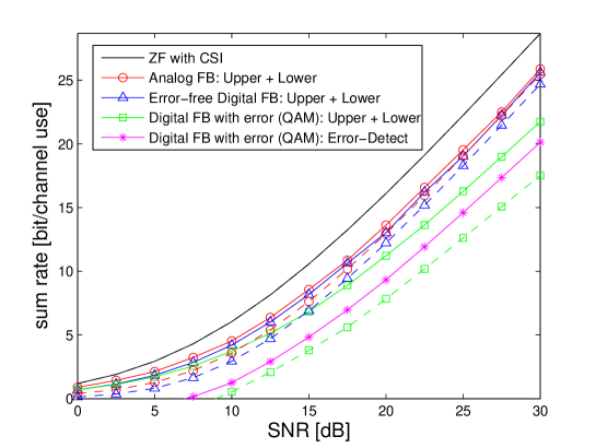
Figure 2: Achievable rate lower (dotted lines) and upper (solid lines) bounds for analog, error-free digital, and QAM-based digital feedback for $M=4$ and $\beta_{\rm fb}=1$.

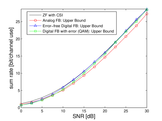
Figure 3: Achievable rate upper bounds for analog, error-free digital, and QAM-based digital feedback for $M=4$ and $\beta_{\rm fb}=2$.

Figure 4: Achievable rate lower (dotted lines) and upper (solid lines) bounds for analog, error-free digital, and QAM-based digital feedback for $M=4$ and $\frac{P}{N_{0}}=10$ dB and $\frac{P}{N_{0}}=20$ dB.

It is worth noting that the same basic conclusion, i.e., that digital feedback (with or without errors) outperforms analog for sufficiently large $\beta_{\rm fb}$, also holds in the presence imperfect CSIR. However, because imperfect CSIR leads to a residual term in the rate gap expression that does not vanish (even for large $\frac{P}{N_{0}}$), the absolute difference between digital and analog feedback is reduced.

V Channel state feedback over the MIMO-MAC

Orthogonal access in the feedback link requires $O(M^{2})$ channel uses for the feedback, while the downlink capacity scales at best as $O(M)$. When the number of antennas $M$ grows large, such a system would not scale well with $M$. On the other hand, the inherent MIMO-MAC nature of the physical uplink channel suggests an alternative approach, where multiple UT’s simultaneously transmit on the MIMO uplink (feedback) channel and the spatial dimension is exploited for channel state feedback too. This idea was considered for an FDD system in [28] and analyzed in terms of the mean square error of the channel estimate provided to the BS.

As in [28], we partition the $M$ users into $\frac{M}{L}$ groups of size $L$, and let UTs belonging to the same group transmit their feedback signal simultaneously, in the same time frame. Each UT transmits its $M$ channel coefficients over $\beta_{\rm fb}M$ channel uses, with $\beta_{\rm fb}\geq 1$. Therefore, each group uses $\beta_{\rm fb}M$ channel symbols and the total number of channel uses spent in the feedback is $\beta_{\rm fb}\frac{M^{2}}{L}$. Choosing $L\propto M$ (e.g., $L=M/2$) yields a total number of feedback channel uses that grows linearly with $M$, such that the feedback resource converges to a fixed fraction of the downlink capacity. We assume that the uplink feedback channel is affected by i.i.d. block fading (i.e., has the same distribution as the downlink channel) and that there is no feedback delay.

With respect to the analysis provided in [28], the present work differs in a few important aspects: 1) we consider both analog and digital feedback; 2) although our analog feedback model is essentially identical to the FDD scheme of [28], we consider optimal MMSE estimation rather than Least-Squares estimation (zero-forcing pseudo-inverse); 3) we put out results in the context of the rate gap framework, that yields directly fundamental lower bounds on achievable rates, rather than in terms of channel state estimation error.

V-A Analog Feedback

In an analog feedback scheme, each UT feeds back a scaled noisy version of its downlink channel, given by $\frac{\sqrt{\beta_{\rm fb}P}}{\sqrt{\beta_{1}P+N_{0}}}\ {{\bf s}_{k}}$ where ${\bf s}_{k}$ is the observation provided by the common training phase, defined in (4). Due to the symmetry of the problem, we can focus on the simultaneous transmission of a single group of $L$ UTs. Let ${\bf A}=[{\bf a}_{1}~{}\cdots~{}{\bf a}_{L}]\in\mbox{\bb C}^{M\times L}$ denote the uplink fading matrix for this group of UTs (with i.i.d. entries, $\sim{\cal C}{\cal N}(0,1)$) and let for $k=1,\dots,L$

$$b_{k,j}=\frac{\sqrt{\beta_{\rm fb}P}}{\sqrt{\beta_{1}P+N_{0}}}s_{k,j}=\frac{\sqrt{\beta_{\rm fb}\beta_{1}}P}{\sqrt{\beta_{1}P+N_{0}}}h_{k,j}+\frac{\sqrt{\beta_{\rm fb}P}}{\sqrt{\beta_{1}P+N_{0}}}z_{k,j}$$ (46)

denote the transmitted symbol by UT $k$ for its $j$-th channel coefficient, where $s_{k,j}$ is the $j$-th component of ${\bf s}_{k}$ and, from (4), $z_{k,j}$ is the common training AWGN. For simplicity, we assume that the BS has perfect knowledge of the uplink channel state ${\bf A}$; we later consider the more general case and see that the main conclusions are unchanged.

The $M$-dimensional received vector ${\bf g}_{j}$, upon which the BS estimates the $j$-th antenna downlink channel coefficients $h_{1,j},\ldots,h_{L,j}$ of all users in the group, is given by:

$${\bf g}_{j} = \sum_{i=1}^{L}{\bf a}_{i}b_{i,j}+\widetilde{{\bf w}}_{j}={\bf A}{\bf b}_{j}+\widetilde{{\bf w}}_{j}$$ (47)

where $\widetilde{{\bf w}}_{j}$ is an AWGN vector with i.i.d. elements $\sim{\cal C}{\cal N}(0,N_{0})$. From the i.i.d. jointly Gaussian statistics of the channel coefficients, downlink noise and uplink (feedback noise) it is immediate to obtain the MMSE estimator for the downlink channel coefficient $h_{k,j}$ in the form

$$\widehat{h}_{k,j}=c\ {\bf a}_{k}^{\sf H}\left[\beta_{\rm fb}P{\bf A}{\bf A}^{\sf H}+N_{0}{\bf I}\right]^{-1}{\bf g}_{j}$$ (48)

where we define the constant $c=\frac{\sqrt{\beta_{\rm fb}\beta_{1}}P}{\sqrt{\beta_{1}P+N_{0}}}$. The corresponding MMSE, for given feedback channel matrix ${\bf A}$, is given by

$$\sigma_{k}^{2}({\bf A})=1-c^{2}{\bf a}_{k}^{\sf H}\left[\beta_{\rm fb}P{\bf A}{\bf A}^{\sf H}+N_{0}{\bf I}\right]^{-1}{\bf a}_{k}$$ (49)

Theorem 7

If each UT feeds back its channel coefficients in analog fashion over the MIMO MAC uplink channel, with groups of $L$ users simultaneously feeding back and $\beta_{\rm fb}M$ channel uses per group, the rate gap upper bound is given by:

$$\overline{\Delta R}^{\textsc{AF}}_{\textsc{MIMO-MAC}}=\log\left(1+\frac{1}{M}\frac{\frac{P}{N_{0}}}{1+\beta_{2}\frac{N_{0}}{P}}+\frac{M-1}{M}\ \frac{P}{N_{0}}\left[\frac{1}{1+\frac{\beta_{1}P}{N_{0}}}+\frac{\frac{\beta_{1}P}{N_{0}}}{1+\frac{\beta_{1}P}{N_{0}}}{\sf mmse}\left(\frac{\beta_{\rm fb}P}{N_{0}}\right)\right]\right)$$ (50)

where we define the average channel state information estimation MMSE as

$${\sf mmse}(\rho)\triangleq\frac{1}{L}\sum_{k=1}^{L}\mbox{\bb E}\left[\frac{1}{1+\rho\lambda_{k}}\right]$$ (51)

and where $\{\lambda_{1},\ldots,\lambda_{L}\}$ denote the eigenvalues of the $L\times L$ central Wishart matrix ${\bf A}^{\sf H}{\bf A}$.

Furthermore, if $L<M$ the rate gap is bounded and converges at high SNR to the constant

$$\lim_{P/N_{0}\rightarrow\infty}\overline{\Delta R}^{\textsc{AF}}_{\textsc{MIMO-MAC}}=\log\left(1+\frac{1}{\beta_{2}M}+\frac{M-1}{M}\left(\frac{1}{\beta_{1}}+\frac{1}{\beta_{\rm fb}(M-L)}\right)\right).$$ (52)

Proof: See Appendix F. ∎

Comparing this expression to the rate gap for analog feedback over an AWGN channel (30), we notice that an SNR (array) gain of $M-L$ is achieved (on the feedback channel) when the feedback is performed over the MIMO MAC because the feedback (of $L$ users) is received over $M$ antennas. In addition, a factor of $L$ fewer feedback symbols are required when the feedback is performed over the MIMO MAC ($\beta_{\rm fb}\frac{M^{2}}{L}$ vs. $\beta_{\rm fb}M^{2}$). On the other hand, using the second line of the RHS of (89) in Appendix C it is immediate to show that for $L=M$ the rate gap upper bound grows unbounded as $\log\log\left(\frac{P}{N_{0}}\right)$.

From (52) we can optimize the value of $L$ (assuming $L<M$) for a fixed number of feedback channel uses, which we denote by $aM$ for some $a\geq 2$ (if $L<M$ there must be at least two groups and thus we must have at least $2M$ feedback symbols). By letting $aM=\beta_{\rm fb}\frac{M^{2}}{L}$, we obtain $\beta_{\rm fb}=a\frac{L}{M}$. Using this in (52), we have that minimizing the rate gap bound is equivalent to maximizing the term $L(M-L)$ for fixed $M$ and $L<M$. Therefore, the optimal group size is given by $L^{*}=\frac{M}{2}$. Substituting this value in (52) yields

$$\log\left(1+\frac{1}{\beta_{2}M}+\frac{2(M-1)}{M^{2}\beta_{\rm fb}}+\frac{M-1}{M}\frac{1}{\beta_{1}}\right)$$ (53)

and the corresponding total number of feedback symbols is $2\beta_{\rm fb}M$. Interestingly, we notice that in the regime of large $M$ the term that dominates the optimized rate gap bound (53) corresponds to the downlink common training phase. In fact, the terms corresponding to dedicated training and feedback vanish as $M$ increases.

When the total number of feedback symbols is larger or equal to $2M$ (i.e., $a\geq 2$) numerical results verify that also at finite SNR the choice $L^{*}=\frac{M}{2}$ yields the best performance both in terms of the achievable rate lower bound and of the the genie-aided upper bound. Hence, the optimal MIMO-MAC feedback strategy is a combination of TDMA and SDMA. In contrast, when total number of feedback symbols is strictly smaller than $2M$ (i.e., $1\leq a<2$), choosing $L=M$ with $\beta_{\rm fb}=a$ is the only option. Although this choice yields an unbounded rate gap, it does provide reasonable performance at finite SNR’s.

A legitimate question at this point is the following: is the condition $L<M$ a fundamental limit of the MIMO-MAC analog feedback in order to achieve a bounded rate gap, or is it due to the looseness of Theorem 2? In order to address this question, we examine the genie-aided rate upper bound of Theorem 3 and obtain the following rate upper bound:

Theorem 8

When a group of $L=M$ UTs feed back the channel coefficients simultaneously over $\beta_{\rm fb}M$ channels uses of the fading MIMO-MAC, the difference between $R_{k}^{\rm ZF}$ and the genie-aided upper bound of Theorem 3 is uniformly bounded for all SNRs.

Proof See Appendix G. $\square$

Theorem 8 suggests that if the UTs are able to obtain an estimate of their instantaneous residual interference level in each frame, up to $M$ UTs can feedback their channel state information at the same time. The ability of estimating the interference coefficients ${\cal A}_{k}$ (see (8) and the comment following Theorem 3) depends critically on the quality of the dedicated training. Hence, the dedicated training has a direct impact on the design and efficiency of the channel state feedback. Such inter-dependencies between the different system components can be illuminated thanks to the comprehensive system analysis carried out in this work and are missed by making overly simplifying assumptions (e.g., genie-aided coherent detection with perfect knowledge of the coefficients ${\cal A}_{k}$).

Remark V.1

In [28], the same model in (46) for analog channel state feedback over the MIMO-MAC uplink channel is considered. Instead of the linear MMSE estimator considered here, a zero-forcing approach (via the pseudo-inverse of the matrix ${\bf A}$) is examined. In the case of $L=M$ this yields an infinite error variance, which does not make sense in light of the fact that each channel coefficient has unity variance. This odd behavior can be avoided by performing an additional component-wise MMSE step. As a matter of fact, performance very similar to what we have found for the full MMSE estimator can be obtained for $L<M$ by using a zero-forcing receiver for the channel state feedback, followed by individual (componentwise) MMSE scaling. We omit the analysis of such suboptimal scheme for the sake of brevity. $\lozenge$

Remark V.2

It is also possible to analyze the more realistic scenario where the uplink channel matrix ${\bf A}$ is known imperfectly at the BS. We consider the following simple training-based scheme: the $L$ UTs within a feedback group transmit a preamble of $\beta_{\rm up}L$ training symbols, where $\beta_{\rm up}\geq 1$ defines the uplink training length (per UT). Without repeating all steps in the details, the uplink channel ${\bf A}$ admits the following decomposition:

$${\bf A}=\widehat{{\bf A}}+\widetilde{{\bf A}}$$ (54)

where the channel estimate and estimation error $(\widehat{{\bf A}},\widetilde{{\bf A}})$ are jointly jointly Gaussian and independent, with per-component variances $1-\sigma_{\rm up}^{2}$ and $\sigma_{\rm up}^{2})$, respectively, with $\sigma_{\rm up}^{2}=\frac{1}{1+\beta_{\rm up}\frac{P}{N_{0}}}$. Now, the MMSE estimation of the downlink channel coefficients $h_{k,j}$ is conditional with respect to $\widehat{{\bf A}}$. By repeating all previous steps, after a lengthy calculation that we do not report here for the sake of brevity, we obtain the average estimation error in the form

$$\mbox{\bb E}[\sigma_{k}^{2}(\widehat{{\bf A}})] = \frac{1}{1+\beta_{1}\frac{P}{N_{0}}}+\frac{\beta_{1}\frac{P}{N_{0}}}{1+\beta_{1}\frac{P}{N_{0}}}\ {\sf mmse}\left(\frac{\beta_{\rm up}\frac{P}{N_{0}}}{1+\beta_{\rm up}\frac{P}{N_{0}}+L\beta_{\rm fb}\frac{P}{N_{0}}}\frac{\beta_{\rm fb}P}{N_{0}}\right)$$ (55)

where ${\sf mmse}(\cdot)$ was defined in (51). By comparing (55) with (87), we notice that they differ only in the argument of the function ${\sf mmse}(\cdot)$. The two expressions coincide for $\beta_{\rm up}\rightarrow\infty$, consistent with the fact that $\beta_{\rm up}\rightarrow\infty$ corresponds to perfect estimation of the channel matrix ${\bf A}$. Furthermore, for large SNR, the two arguments differ by a constant multiplicative factor. Hence, apart from this constant factor that depends on the uplink training parameter $\beta_{\rm up}$, the conclusions about the rate gap obtained for the case of perfect uplink channel knowledge also hold for the case of training-based uplink channel estimation. $\lozenge$

V-B Digital Feedback

In the case of digital feedback, we let $L\leq M$ UTs multiplex their channel state feedback codewords at the same time. The resulting MIMO-MAC channel model is again given by (47), but now the vector ${\bf b}_{j}$ contains the $j$-th symbols of the feedback codewords of the $L$ UTs sharing the same feedback frame. As in Section IV-B, we assume that feedback messages of $\alpha(M-1)\log_{2}\frac{P}{N_{0}}$ bits are sent in $\beta_{\rm fb}(M-1)$ channel uses. Hence, the feedback symbols transmitted by the $L$ UT’s can be grouped in a $L\times\beta_{\rm fb}(M-1)$ matrix, while the BS has an $M\times\beta_{\rm fb}(M-1)$ observation upon which to estimate the transmitted symbols. We again assume each feedback symbol has average energy $P$.

Suppose that the BS receiver operates optimally, by using a joint ML decoder for all the simultaneously transmitting UTs. The high-SNR error probability performance of the MIMO-MAC channel was characterized in terms of the diversity-multiplexing tradeoff in [56]. In particular, when each user transmits at rate $r\log_{2}\frac{P}{N_{0}}$ bits/symbol (i.e., with multiplexing gain $r$) over the MIMO-MAC with i.i.d. channel fading (as considered here), the optimal ML decoder achieves an individual user average error probability

$$P_{e,{\rm fb}}\;\doteq\;\left(\frac{P}{N_{0}}\right)^{-d^{*}(r)}$$

where the “dot-equality” notation, introduced in [57, 56], indicates that $\lim_{P/N_{0}\rightarrow\infty}\frac{-\log P_{e,{\rm fb}}}{\log P/N_{0}}=d^{*}(r)$. The error probability SNR exponent $d^{*}(r)$ is referred to as the optimal diversity gain of the system. Particularizing the results of [56] to the case of $L\leq M$ users with 1 antenna each, transmitting to a receiver with $M$ antennas, the optimal diversity gain is given by

$$d^{*}(r)=\left\{\begin{array}[]{ll}M(1-r)&\mbox{for}\;\;0\leq r\leq 1\\ 0&\mbox{otherwise}\end{array}\right.$$ (56)

This is the same exponent of a channel with a single user with a single antenna, transmitting to a receiver with $M$ antennas (single-input multiple-output with receiver antenna diversity). In other words, under our system parameters, each UT achieves an error probability that decays with SNR as if TDMA on the feedback link was used (as if the UT transmitted its feedback message alone on the MIMO uplink channel). From what is said above, it follows that the multiplexing gain of all UTs is given by $r=\frac{\alpha}{\beta_{\rm fb}}$. Furthermore, from the derivation of Section IV-C, we require that $1<\alpha<\beta_{\rm fb}$. It follows that the average feedback error message probability in the MIMO-MAC fading channel is given by

$$P_{e,{\rm fb}}=\left(\frac{P}{N_{0}}\right)^{-M(1-\alpha/\beta_{\rm fb})}\times g\left(\frac{P}{N_{0}}\right)$$ (57)

where $g(x)$ is some sub-polynomial function, such that $\lim_{x\rightarrow\infty}x^{-\epsilon}g(x)=0$ for all fixed $\epsilon>0$.

If we examine the rate-gap expression with digital feedback (42), we see that in order to achieve a bounded rate gap the error probability $P_{e,{\rm fb}}$ must go to zero at least as fast as $\left(\frac{P}{N_{0}}\right)^{-1}$. From (57) we have that for all $1<\alpha<\beta_{\rm fb}$ such that $M(1-\alpha/\beta_{\rm fb})$ is strictly larger than 1, the resulting rate gap is bounded and the effect of feedback errors vanishes. This imposes the condition $\beta_{\rm fb}>\frac{M}{M-1}$ and $\alpha<\frac{M-1}{M}\beta_{\rm fb}$, which is stricter than the condition $\beta_{\rm fb}>1$ and $\alpha<\beta_{\rm fb}$ needed in the case of TDMA an unfaded feedback channel previously analyzed in Section IV-C.

We conclude that a bounded rate gap can also be achieved with digital feedback on the MIMO-MAC uplink channel. Therefore, also in this case we can achieve a number of feedback channel uses that scales linearly with the number of the BS antennas $M$. Explicit design of codes that achieve the optimal divesity-multiplexing tradeoff of MIMO-MAC channels is not an easy task in general. In the particular case of $M$ users with one antenna each, simple explicit constructions of MIMO-MAC codes for the digital channel state feedback are presented [53]. These codes can be optimally decoded by using a Sphere Decoder [58, 59] and achieve the performance promised by the above analysis. It should be noticed, however, that while in the AWGN case the term $\frac{P}{N_{0}}P_{e,{\rm fb}}$ in the rate gap expression vanishes rapidly (faster than polynomially, in $P/N_{0}$), in the MIMO-MAC fading case it vanishes only as $(P/N_{0})^{1-M(1-\alpha/\beta_{\rm fb})}$. Thus, for finite SNR the rate gap may be significantly larger than in the case of unfaded feedback channel and the optimal tradeoff between quantization distortion and the feedback error probability must be sought by careful optimization of the parameters $\alpha$ and $\beta_{\rm fb}$ (see details in [60]). Also, the same observations about detecting feedback errors at the UTs and discarding the corresponding frames made at the end of Section IV-C apply here.

V-C Numerical example

Fig. 5 shows both the genie-aided upper bound of Theorem 3 and the lower bound based on (50) of analog feedback over a fading MIMO-MAC for $M=4$ and $L=2,4$. We assume perfect CSIR. We notice that for $L=2$, the lower bound coincides with the genie-aided upper bound and comes very close to the performance of ZF with ideal CSIT. For $L=M$, the rate gap of the lower bound (50) is unbounded but the double logarithmic growth $\log\log(P/N_{0})$ yields a very small gap for a wide range of practical SNRs. The genie-aided bound achieves a constant rate gap even for $L=M$, in accordance with Theorem 8. Although not shown here, a system using $M=4,L=2$ and $\beta_{\rm fb}=1$ does outperform $M=L=4$, $\beta_{\rm fb}=2$ (both configurations use a total of $8$ feedback symbols per frame) in terms of the lower bound and the genie-aided upper bound throughout the SNR range shown; this validates our earlier claim about the optimality of $L=\frac{M}{2}$ whenever at least $2M$ feedback symbols are used.

Fig. 6 compares the achievable rates of analog and digital feedback schemes based on the rate gap (50), (42), over a fading MIMO-MAC for $M=4$. For the digital feedback we assume that there exist some code achieving the outage probability (57) with $g(P/N_{0})=1$. We compare both schemes for the same total amount of the feedback symbols (24 symbols). For the analog feedback we choose $L=2,\beta_{\rm fb}=3$, while for the digital feedback we let $L=4,\beta_{\rm fb}=8,\alpha=4$. We observe that the digital feedback achieves near-optimal sum rate over the all SNR ranges while the analog feedback achieves a constant gap of roughly 0.7 bit/channel use. Surprisingly, the digital feedback is able to let M users transmit simultaneously while vanishing both the quantization error and the feedback error.

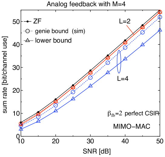
Figure 5: Impact of $L$ with analog feedback over MIMO-MAC

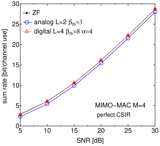
Figure 6: Achievable rate lower bounds for analog and digital feedback for $M=4$ and $24$ total feedback symbols.

VI Effects of CSIT feedback delay

In this section we wish to take into account the effect of feedback delay in a setting where the fading is temporally correlated. We assume that the fading is constant within each frame, but changes from frame to frame according to a stationary random process. In particular, assuming spatial independence, each entry of ${\bf h}_{k}$ evolves independently according to the same complex circularly symmetric Gaussian stationary ergodic random process, denoted by $\{h(t)\}$, with mean zero, unit variance and power spectral density (Doppler spectrum) denoted by $S_{h}(\xi)$, $\xi\in[-1/2,1/2]$, and satisfying $\int_{-1/2}^{1/2}S_{h}(\xi)d\xi=1$, Notice that the discrete-time process $\{h(t)\}$ has time that ticks at the frame rate.

Because of symmetry and spatial independence, we can neglect the UT index $k$ and the antenna index and consider scalar rather than vector processes. Generalizing (4), the observation available at each UT at time $t-d$ from the common training phase takes on the form

$$\left\{s(t-\tau)=\sqrt{\beta_{1}P}h(t-\tau)+z(t-\tau):\tau=d,d+1,d+2,\ldots,\infty\right\}$$ (58)

where $d$ indicates the feedback delay in frames. This means that the channel state feedback to be used by the BS at frame time $t$ is formed from noisy observations of the channel up to time $t-d$. We consider a scheme where each UT at frame $t-d$ produces the MMSE estimate of its channel at frame $t$ and sends this estimate (using either analog or digital feedback) to the BS; the BS uses the received feedback to choose the beamforming vectors used for data transmission in frame $t$.

VI-A Estimation Error at UT

The key quantity in the associated rate gap is the MMSE prediction error at the UT. Let $\widetilde{h}(t)$ denote the MMSE estimate of $h(t)$ given the observations in (58). Given the joint Gaussianity of $h$ and $s$, we can write

$$h(t)=\widetilde{h}(t)+n(t)$$ (59)

where $\mbox{\bb E}[|n(t)|^{2}]=\sigma_{1}^{2}$ is the estimation MMSE, and $\widetilde{h}(t)$ and $n(t)$ are independent with $\mbox{\bb E}[|\widetilde{h}(t)|^{2}]=1-\sigma_{1}^{2}$. From classical Wiener filtering theory [46], the one-step prediction ($d=1$) MMSE error is given by

$$\epsilon_{1}(\delta)=\exp\left(\int_{-1/2}^{1/2}\log(\delta+S_{h}(\xi))d\xi\right)-\delta$$ (60)

where $\delta=N_{0}/(\beta_{1}P)$ is the observation noise variance. The filtering MMSE ($d=0$) is related to $\epsilon_{1}(\delta)$ as

$$\epsilon_{0}(\delta)=\frac{\delta\epsilon_{1}(\delta)}{\delta+\epsilon_{1}(\delta)}.$$ (61)

The scenario considered in all previous sections corresponds to i.i.d. fading (across blocks) and $d=0$, in which case $\epsilon_{1}(\delta)=1$ (past observations are useless) and thus $\sigma_{1}^{2}=\epsilon_{0}(\delta)=(1+\beta_{1}\frac{P}{N_{0}})^{-1}$, which coincides with (7). More in general, in this section we shall consider  $\sigma_{1}^{2}=\epsilon_{d}(\delta)$ for $d=0,1$.

We distinguish two cases of channel fading statistics: Doppler process and regular process:

• We say that $\{h(t)\}$ is a Doppler process if $S_{h}(\xi)$ is strictly band-limited to $[-F,F]$, where $F<1/2$ is the maximum Doppler frequency shift, given by $F=\frac{vf_{c}}{c}T_{f}$, where $v$ is the mobile terminal speed (m/s), $f_{c}$ is the carrier frequency (Hz), $c$ is light speed (m/s) and $T_{f}$ is the frame duration (s) [40]. A Doppler process satisfies $\int_{-F}^{F}\log S_{h}(\xi)d\xi>-\infty$, and has prediction error

  $$\epsilon_{1}(\delta)=\delta^{1-2F}\exp\left(\int_{-F}^{F}\log(\delta+S_{h}(\xi))d\xi\right)-\delta$$ (62)

  Therefore, $\lim_{\delta\rightarrow 0}\epsilon_{1}(\delta)=0$.

• We say that $\{h(t)\}$ is a regular process if $\epsilon_{1}(0)>0$ (see [39] and references therein). In particular, a process satisfying the Paley-Wiener condition [46] $\int_{-1/2}^{1/2}\log S_{h}(\xi)d\xi>-\infty$ is regular.

For the case of no delay ($d=0$), for either type of process the estimation error goes to zero with the observation noise, i.e., $\epsilon_{0}(\delta)\rightarrow 0$ as $\delta\rightarrow 0$. However, they differ sharply in terms of prediction error: $\epsilon_{1}(\delta)$ is strictly positive for a regular process (even as $\delta\rightarrow 0$), whereas $\epsilon_{1}(\delta)\rightarrow 0$ for Doppler processes as quantified in the following:

Lemma 1

The noisy prediction error of a Doppler process satisfies

$$\epsilon_{1}(\delta)=\kappa\delta^{1-2F}+O(\delta)$$ (63)

for $\delta\downarrow 0$, where $\kappa$ is a constant term independent of $\delta$.

Proof: Applying Jensen’s inequality to (62) from the fact that $\int S_{h}(\xi)d\xi=1$, we obtain the upper bound

$$\epsilon_{1}\left(\delta\right)\leq\delta^{1-2F}\left[\left(\frac{1}{2F}+\delta\right)^{2F}-\delta^{2F}\right]$$ (64)

Using the fact that $\log$ is increasing, we arrive at the lower bound

$$\epsilon_{1}\left(\delta\right)\geq\delta^{1-2F}\left[\exp\left(\int_{-F}^{F}\log S_{h}(\xi)d\xi\right)-\delta^{2F}\right]$$ (65)

Combining these bounds we obtain the result. ∎

VI-B Rate Gap Upper Bound

When analog feedback is used, each UT transmits a scaled version of its MMSE estimate $\widetilde{h}(t)$ over the feedback channel. The only difference from the scenarios studied in Sections V-A (AWGN feedback channel) and IV-A (MIMO MAC feedback channel) is that the estimation error at the UT is $\epsilon_{d}\left(N_{0}/(\beta_{1}P)\right)$ rather than $(1+\beta_{1}P/N_{0})^{-1}$. As a result, a simple calculation confirms that the expressions for the rate gap upper bound given in Theorems 4 (AWGN) and 7 (MIMO-MAC) apply to the present if $\epsilon_{d}\left(N_{0}/(\beta_{1}P)\right)$ is substituted for $(1+\beta_{1}P/N_{0})^{-1}$. The same equivalence holds for digital feedback: each UT quantizes its MMSE estimate $\widetilde{h}(t)$, and as a result the rate gap upper bound given in Theorem 5 applies with the same substitution. For the sake of brevity, the expressions for the rate gap upper bound are not provided here.

In fact, the effect of feedback delay is most clearly illustrated by considering perfect feedback (i.e., $\beta_{\rm fb}\rightarrow\infty$), in which case (at frame $t$) the BS has perfect knowledge of $\widetilde{h}(t)$, the UT’s prediction of $h(t)$ based on common training observations up to frame $t-d$. For the sake of simplicity we further assume perfect dedicated training (i.e., $\beta_{2}\rightarrow\infty$), in which case the rate gap upper bound is

$$\overline{\Delta R}^{\textsc{predict}}=\log\left(1+\frac{P}{N_{0}}\frac{M-1}{M}\epsilon_{d}\left(\frac{N_{0}}{\beta_{1}P}\right)\right).$$ (66)

We now analyze the cases of no delay and one-step delay for both types of processes.

No feedback delay ($d=0$)

Because using past observations can only help, the filtering error is no larger than the error if the past is ignored, i.e., $\epsilon_{0}\left(\delta\right)\leq(1+\beta_{1}P/N_{0})^{-1}$. It thus follows that for both Doppler and regular processes the rate gap is bounded. Based upon (61), Lemma 1, and the property $\epsilon_{0}(0)>0$ for regular processes, it is straightforward to see that $(P/N_{0})\epsilon_{0}\left(N_{0}/(\beta_{1}P)\right)\rightarrow\frac{1}{\beta_{1}}$ as $\frac{P}{N_{0}}\rightarrow\infty$ for either regular or Doppler processes. As a result, the rate gap upper bound in (66) converges to $\log(1+1/\beta_{1})$ at high SNR. This matches the high SNR expression for block-by-block estimation in (30), showing that filtering does not provide a significant advantage at asymptotically high SNR. However, as later illustrated through numerical results, this convergence occurs extremely slowly for Doppler processes or highly correlated regular processes, in which case filtering does provide a non-negligible gain over a wide range of SNR’s.

Feedback delay ($d=1$)

For regular fading process, since $\epsilon_{1}(0)>0$, the quantity $(P/N_{0})\epsilon_{1}\left(N_{0}/(\beta_{1}P)\right)$ increases linearly with $\frac{P}{N_{0}}$ and thus the rate gap upper bound $\overline{\Delta R}^{\textsc{predict}}$ grows like $\log\frac{P}{N_{0}}$. As a result, the achievable rate lower bound $R_{k}^{\textrm{Z}F}-\overline{\Delta R}^{\textsc{predict}}$ is bounded even as $P/N_{0}\rightarrow\infty$. In addition, in Appendix H we show that the genie-aided upper bound is also bounded due to the fundamentally non-deterministic nature of regular processes. This shows that with delayed feedback and a channel that evolves according to a regular fading process, a system that makes use of zero-forcing naive beamforming to $M$ users becomes interference limited. This behavior holds even with CSIR (i.e., letting $\beta_{1}\rightarrow\infty$).

Fortunately, physically meaningful fading processes belong to the class of Doppler processes, at least over a time-span where they can be considered stationary. For a practical relative speed between BS and UT, such time span is much larger than any reasonable coding block length. Hence, we may say that Doppler processes are more the rule than the exception. In this case, the system behavior is radically different. Using Lemma 1, at high SNR the rate gap upper bound is

$$\log\left(1+\frac{M-1}{M}\frac{P}{N_{0}}\left(\kappa\left(\frac{\beta_{1}P}{N_{0}}\right)^{2F-1}+O\left(\frac{N_{0}}{\beta_{1}P}\right)\right)\right),$$ (67)

and thus the rate gap grows like $2F\log\frac{P}{N_{0}}$. Using this in the rate lower bound of Corollary (III.1), and considering the pre-log factor in high-SNR, we have that the system sum-rate is lowerbounded by

$$\sum_{k=1}^{M}R_{k}\geq M(1-2F)\log\frac{P}{N_{0}}+O(1)$$ (68)

This shows that a multiplexing gain of $M(1-2F)$ is achievable.

Remark VI.1

If perfect CSIR is assumed, an interesting singularity is observed for Doppler processes. Under this assumption each UT is able to perform perfect prediction of its channel state on the basis of its past noiseless observations of the channel, by the definition of a Doppler process. Thus, it is as if there is no delay and the full multiplexing gain of $M$ is achieved (even if the feedback link is imperfect). On the other hand, if perfect CSIR is not assumed and UT’s learn their channel through $\beta_{1}M$ common training symbols, for any finite value of $\beta_{1}$ a multiplexing gain of only $M(1-2F)$ is achieved. This point illustrates, again, that neglecting some system aspects may yield to erroneous conclusions. In this case, by properly modeling imperfect CSIR we have illuminated the impact of the UTs speed (which determines the channel Doppler bandwidth ) on the system achievable rates in a concise and elegant way. $\lozenge$

Remark VI.2

It is interesting to notice here the parallel with the results of [39] on the high-SNR capacity of the single-user scalar ergodic stationary fading channel with no CSIR and no CSIT, where it is shown that for a class of non-regular processes that includes the Doppler processes defined here, the high-SNR capacity grows like ${\cal L}\log(P/N_{0})$, where ${\cal L}$ is the Lebesgue measure of the set $\{\xi\in[-1/2,1/2]:S_{h}(\xi)=0\}$. In our case, it is clear that ${\cal L}=1-2F$. These results, as ours, rely on the behavior of the noisy prediction error $\epsilon_{1}(\delta)$ for small $\delta$. $\lozenge$

VI-C Examples

We now present numerical results for the Jake’s model and the Gauss-Markov model, which are two widely used Doppler and regular processes, respectively. The classical Jakes’ correlation model has the following spectrum [62, 54]

$$S_{h}(\xi)=\frac{1}{\pi\sqrt{F^{2}-\xi^{2}}},\;\;\;-F\leq\xi\leq F,$$ (69)

and auto-correlation function $J_{0}(2\pi F\tau)$. No closed-form solution is known for the prediction or filtering error. Under the Gauss-Markov model (i.e., auto regressive of order 1) the channel evolves in time as:

$$h(\tau)=rh(\tau-1)+\sqrt{1-r^{2}}\Delta(\tau)$$ (70)

where $r$ is the correlation coefficient ($0<r<1$) and the innovation process $\Delta(\tau)$ is unit-variance complex Gaussian, i.i.d. in time. The prediction error for such model can be written in closed-form and is given by (see for example [32])

$$\epsilon_{1}(\delta) = (1-r^{2})\left[1+\frac{-(1+\delta)+\sqrt{1+\delta^{2}+2\delta\frac{1+r^{2}}{1-r^{2}}}}{2}\right]$$ (71)

For the Jakes’ model we have $F=\frac{vf_{c}}{c}T_{f}$. In all results we consider $f_{c}=2$ GHz and $T_{f}=1$ msec. Motivated by the maximum-entropy principle [63], several works in wireless communication modeled channel fading as Gauss-Markov process with one-step correlation coefficient $r=J_{0}(2\pi F)$, given by Jakes’ model. Comparing the performance of the true Jakes’ model with its Gauss-Markov maximum-entropy approximation, we will point out that the latter may be overly pessimistic for high-speed mobile terminals.

In Fig. 7 the achievable rate lower bound with delay-free feedback ($d=0$) and optimal filtering is plotted versus SNR for the Jakes and Gauss-Markov models, for $M=4$, $v=10$ km/hr ($F=0.0185$ and $r=0.9966$), and $\beta_{1}=1$. Filtering is seen to provide an advantage with respect to block-by-block estimation for a wide range of SNR’s. For the Gauss-Markov model this advantage vanishes around 30 dB, whereas for Jakes’ model this advantage persists far beyond the range of this plot.

Using the same parameters, in Fig. 8 we plot the lower bound for one-step prediction ($d=1$) versus SNR for $v=3$ and $10$ km/hr ($F=0.0056$ and $F=0.0185$). This figure illustrates the contrast between Doppler and regular processes: for Jakes’ model the achieved rate is quite close to the perfect channel state information rate (although a slight loss in multiplexing gain is evident), whereas the rate for the Gauss-Markov model saturates at sufficiently high SNR due to the unpredictability inherent to the model. To further emphasize the difference in behavior, in Fig. 9 we plot the lower bound for one-step prediction ($d=1$) versus $\beta_{1}$, the number of common training symbols per block, for $P/N_{0}=10$ and $15$ dB and $v=10$ km/hr. As $\beta_{1}$ increases (and thus the observation noise decreases) the rate for Jakes’ model converges to the ideal case. On the other hand, the rate for the Gauss-Markov model saturates at a rate strictly smaller than the ideal channel state information rate because there is strictly positive prediction error even if noiseless past observations (i.e., $\beta_{1}\rightarrow\infty$) are provided.

In conclusion, the most noteworthy result of this analysis is that under common fading models (Doppler processes), both analog and digital feedback scheme achieves a potentially high multiplexing gain even with realistic, noisy and delayed feedback.

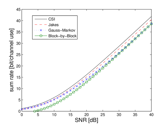
Figure 7: Achievable rate lower bounds with optimal filtering for the Jake’s and Gauss-Markov models for $M=4$ and $v=10$ km/hr ($F=0.0185$ and $r=0.9966$). Also shown are the rates with perfect CSI and with block-by-block estimation.

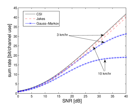
Figure 8: Achievable rate lower bounds with optimal one-step prediction for the Jake’s and Gauss-Markov models for $M=4$.

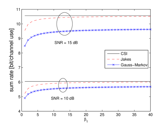
Figure 9: Achievable rate lower bounds with optimal one-step prediction versus $\beta_{1}$ for $M=4$ and $v=10$ km/hr.

VII Conclusions

This paper presents a comprehensive and rigorous analysis of the achievable performance of ZF beamforming under pilot-based channel estimation and explicit channel state feedback. We considered what we believe are the most relevant system aspects. In particular, the often neglected effect of explicit channel estimation at the UTs is taken into account, including both common training and dedicated training phases. As for the feedback, our closed-form bounds allow for a detailed comparison of analog and digital feedback schemes, including the effects of the MIMO-MAC fading channel, of digital feedback decoding errors, and of feedback delay.

Our results build on prior work, but generalize many results and models. We have focused on the case of FDD, but our results easily extend to TDD systems with channel reciprocity. It is perhaps important to point out here that our results show that, even in the case of FDD, a system with explicit CSIT feedback can be implemented, where the number of training and feedback channel uses scales linearly with the number of BS antennas, and eventually with the downlink throughput.

The throughput of the system analyzed here can be improved via the use of combined beamforming and user selection/scheduling. Simulation results show that a system with $K=10$ and $M=4$, with a greedy scheduling as proposed in [15, 32], achieves a very small gap with respect to the optimal dirty-paper coding and perfect CSIT case with the same parameters. Although a clean closed-form analytical characterization of a system with beamforming and user selection based on imperfect channel state information appears to be difficult, recent results [33, 45] indicate that the dependence on CSIT quality when user selection is performed is roughly the same as the equal-power/no selection scenario analyzed here.

We would like to conclude by noticing that some practically relevant extensions of the present work have been presented (by the same authors and by others) since the submission of this paper. In particular, the rate gap analysis was extended to the very relevant case of MIMO OFDM with frequency-correlated fading in [52], the optimal allocation of training and feedback resources is considered in [37, 38], explicit coding schemes for the CSIT digital feedback MIMO-MAC channel are presented in [53], and comparisons between single-user and multi-user MIMO (based on the bounds developed here and related approximations) are performed in [64].

Appendix A Proof of Theorem 1

The proof is closely inspired by that of Lemma B.0.1 of [36]. First, notice that since $\widehat{a}_{k,k}$ is a function of ${\cal R}_{k}$, by the data-processing inequality we have that

$$I(u_{k};y_{k},{\cal R}_{k})\geq I(u_{k};y_{k},\widehat{a}_{k,k})$$

Then, because $I(u_{k};y_{k},\widehat{a}_{k,k})=h(u_{k})-h(u_{k}|y_{k},\widehat{a}_{k,k})$ and $h(u_{k})=\log\left(\pi e\frac{P}{M}\right)$, a lower bound on mutual information is derived by upper bounding $h(u_{k}|y_{k},\widehat{a}_{k,k})$ as follows:

$$h(u_{k}|y_{k},\widehat{a}_{k,k}) \mathop{=}\limits^{\rm(a)} h(u_{k}-\alpha\ y_{k}|y_{k},\widehat{a}_{k,k})$$ (72)

$$\mathop{\leq}\limits^{\rm(b)} h(u_{k}-\alpha\ y_{k}|\widehat{a}_{k,k})$$

$$\mathop{\leq}\limits^{\rm(c)} \mbox{\bb E}\left[\log\left(\pi e\cdot\mbox{\bb E}\left[|u_{k}-\alpha\ y_{k}|^{2}|\widehat{a}_{k,k}\right]\right)\right]$$

where ${\rm(a)}$ holds for any deterministic function $\alpha$ of $y_{k}$ and $\widehat{a}_{k,k}$, ${\rm(b)}$ follows from the fact that conditioning reduces entropy and ${\rm(c)}$ follows by the fact that differential entropy is maximized by a Gaussian RV with the same second moment. Substituting (12) in (8) we have

$$y_{k}=(\widehat{a}_{k,k}+f_{k})u_{k}+I_{k}+z_{k}$$ (73)

where $\widehat{a}_{k,k}u_{k}$ and $f_{k}u_{k}+I_{k}+z_{k}$ are uncorrelated and zero-mean, even if we condition on $\widehat{a}_{k,k}$, because $\widehat{a}_{k,k},f_{k},u_{1},\ldots,u_{K},z_{k}$ are independent, zero-mean Gaussian’s. Thus, we have

$$\mbox{\bb E}\left[|y_{k}|^{2}\ |\widehat{a}_{k,k}\right]=|\widehat{a}_{k,k}|^{2}\mbox{\bb E}[|u_{k}|^{2}]+\sigma^{2}_{2}\ \mbox{\bb E}[|u_{k}|^{2}]+\mbox{\bb E}\left[|I_{k}|^{2}|\widehat{a}_{k,k}\right]+N_{0},$$ (74)

Choosing $\alpha$ that minimizes $\mbox{\bb E}\left[|u_{k}-\alpha\ y_{k}|^{2}|\widehat{a}_{k,k}\right]$ tightens the bound. This corresponds to setting $\alpha\ y_{k}$ equal to the linear MMSE estimate of $u_{k}$ given $y_{k}$ and $\widehat{a}_{k,k}$, i.e.,

$$\alpha=\frac{\mbox{\bb E}\left[u_{k}y_{k}^{*}\ |\ \widehat{a}_{k,k}\right]}{\mbox{\bb E}\left[|y_{k}|^{2}\ |\ \widehat{a}_{k,k}\right]}=\frac{\mbox{\bb E}[|u_{k}|^{2}]\widehat{a}_{k,k}^{*}}{\mbox{\bb E}\left[|y_{k}|^{2}\ |\ \widehat{a}_{k,k}\right]}$$ (75)

Using (74), the corresponding MMSE is given by

$$\mbox{\bb E}\left[|u_{k}-\alpha\ y_{k}|^{2}|\widehat{a}_{k,k}\right] = \mbox{\bb E}\left[|u_{k}|^{2}\right]\left(1-\frac{\mbox{\bb E}[|u_{k}|^{2}]|\widehat{a}_{k,k}|^{2}}{\mbox{\bb E}\left[|y_{k}|^{2}\ |\ \widehat{a}_{k,k}\right]}\right)$$ (76)

$$= \frac{P}{M}\frac{1+\sigma_{2}^{2}\frac{P}{N_{0}M}+\mbox{\bb E}\left[|I_{k}|^{2}|\widehat{a}_{k,k}\right]/N_{0}}{|\widehat{a}_{k,k}|^{2}\frac{P}{N_{0}M}+1+\sigma_{2}^{2}\frac{P}{N_{0}M}+\mbox{\bb E}\left[|I_{k}|^{2}|\widehat{a}_{k,k}\right]/N_{0}}$$ (77)

Replacing (77) into (72) and using $h(u_{k})=\log\left(\pi e\frac{P}{M}\right)$, we obtain (14).

Appendix B Proof of Theorem 2

Using the lower bound on $R_{k}$ from Theorem 1 we have:

$$\Delta R \leq \mbox{\bb E}\left[\log\left(1+\frac{|{\bf h}^{\sf H}{\bf v}_{k}|^{2}P}{N_{0}M}\right)\right]-\mbox{\bb E}\left[\log\left(1+\frac{|\widehat{a}_{k,k}|^{2}P/(N_{0}M)}{1+\sigma_{2}^{2}P/(N_{0}M)+\mbox{\bb E}\left[|I_{k}|^{2}|\widehat{a}_{k,k}\right]/N_{0}}\right)\right]$$ (78)

$$\mathop{\leq}\limits^{\rm(a)} \mbox{\bb E}\left[\log\left(1+\frac{|{\bf h}^{\sf H}{\bf v}_{k}|^{2}P}{N_{0}M}\right)\right]-\mbox{\bb E}\left[\log\left(1+\frac{P}{N_{0}M}\left(|\widehat{a}_{k,k}|^{2}+\sigma_{2}^{2}\right)\right)\right]$$

$$\qquad\qquad\qquad\qquad\qquad\ \ +\ \mbox{\bb E}\left[\log\left(1+\sigma_{2}^{2}\frac{P}{N_{0}M}+\frac{\mbox{\bb E}\left[|I_{k}|^{2}|\widehat{a}_{k,k}\right]}{N_{0}}\right)\right]$$

$$\mathop{\leq}\limits^{\rm(b)} \mbox{\bb E}\left[\log\left(1+\sigma_{2}^{2}\frac{P}{N_{0}M}+\frac{\mbox{\bb E}\left[|I_{k}|^{2}|\widehat{a}_{k,k}\right]}{N_{0}}\right)\right]$$

$$\mathop{\leq}\limits^{\rm(c)} \log\left(1+\sigma_{2}^{2}\frac{P}{N_{0}M}+\frac{\mbox{\bb E}[|I_{k}|^{2}]}{N_{0}}\right)$$ (79)

where ${\rm(a)}$ follows by dropping the non-negative term $\mbox{\bb E}\left[|I_{k}|^{2}|\widehat{a}_{k,k}\right]/N_{0}$. Using the fact that ${\bf h}_{k}$ is spatially white and ${\bf v}_{k}$ is selected independent of ${\bf h}_{k}$ (by the ZF procedure), it follows that ${\bf h}_{k}^{\sf H}{\bf v}_{k}$ is $\sim{\cal C}{\cal N}(0,1)$ and $\widehat{a}_{k,k}\sim{\cal C}{\cal N}(0,1-\sigma_{2}^{2})$. Direct application of Lemma 2, which is provided below, with $A=P/(N_{0}M)$, $\lambda=\sigma_{2}^{2}$ and $X=|{\bf h}_{k}^{\sf H}{\bf v}_{k}|^{2}$, thus proves ${\rm(b)}$. Finally, ${\rm(c)}$ follows from the concavity of $\log(\cdot)$ and Jensen’s inequality.

Lemma 2

If $X$ is a non-negative random variable with $\mbox{\bb E}[X]=1$, for any $A>0$ and any $0\leq\lambda\leq 1$:

$$\mbox{\bb E}\left[\log\left(1+XA\right)\right]\leq\mbox{\bb E}\left[\log\left(1+\left(\lambda+(1-\lambda)X\right)A\right)\right].$$ (80)

Proof: For all $0\leq z\leq 1$, define the function

$$\psi(z)=\mbox{\bb E}\left[\log\left(1+zA+(1-z)XA\right)\right].$$ (81)

Then (80) is equivalent to the inequality $\psi(0)\leq\psi(\lambda)$. By the concavity of $\log(\cdot)$ and Jensen’s inequality we have

$$\psi(z) \leq \log\left(1+zA+(1-z)\mbox{\bb E}\left[X\right]A\right)=\psi(1).$$ (82)

In particular, $\psi(0)\leq\psi(1)$. Moreover, $\psi(z)$ is an expectation of the composition of a concave function and a linear function of $z$, and is hence concave [65]. Thus, the concave function $\psi(z)$ for $z\in[0,1]$ lies above the line joining the points $(0,\psi(0))$ and $(1,\psi(1))$. Hence, we have $\psi(0)\leq\psi(\lambda)$ for $\lambda\in[0,1]$, which proves (80). ∎

Appendix C Proof of Theorem 4

Using (18), to compute $\overline{\Delta R}^{\textsc{AF}}$ we only need to find $\mbox{\bb E}\left[|{\bf h}_{k}^{\sf H}\widehat{{\bf v}}_{j}|^{2}\right]$:

$$\mbox{\bb E}\left[|{\bf h}_{k}^{\sf H}\widehat{{\bf v}}_{j}|^{2}\right] \mathop{=}\limits^{\textrm{(a)}} \mbox{\bb E}\left[|\widehat{{\bf h}}_{k}^{\sf H}\widehat{{\bf v}}_{j}+{\bf{\bf e}}_{k}^{\sf H}\widehat{{\bf v}}_{j}|^{2}\right]$$ (83)

$$\mathop{=}\limits^{\textrm{(b)}} \mbox{\bb E}\left[|{\bf{\bf e}}_{k}^{\sf H}\widehat{{\bf v}}_{j}|^{2}\right]$$

$$\mathop{=}\limits^{\textrm{(c)}} \mbox{\bb E}\left[\widehat{{\bf v}}_{j}^{\sf H}\mbox{\bb E}[{\bf{\bf e}}_{k}{\bf{\bf e}}_{k}^{\sf H}]\widehat{{\bf v}}_{j}\right]$$

$$\mathop{=}\limits^{\textrm{(d)}} \sigma_{e}^{2}$$

where ${\rm(a)}$ follows from (27), ${\rm(b)}$ follows from the fact that $\widehat{{\bf h}}_{k}^{\sf H}\widehat{{\bf v}}_{j}=0\ \forall\ j\neq k$ by naive ZF, ${\rm(c)}$ is obtained from the independence of ${\bf e}_{k}$ and $\widehat{{\bf v}}_{j}$ ($\widehat{{\bf v}}_{j}$ is a deterministic function of $\{\widehat{{\bf h}}_{i}\}_{i\neq j}$), and (d) follows from $\mbox{\bb E}[{\bf{\bf e}}_{k}{\bf{\bf e}}_{k}^{\sf H}]=\sigma_{e}^{2}{\bf I}$ and $\|\widehat{{\bf v}}_{j}\|=1$.

Appendix D Proof of Theorem 5

To compute the rate gap upper bound, we determine $\mbox{\bb E}\left[|{\bf h}_{k}^{\sf H}\widehat{{\bf v}}_{j}|^{2}\right]$ by writing the channel in terms of the UT channel estimate (which is quantized) and the UT estimation error: ${\bf h}_{k}=\widetilde{{\bf h}}_{k}+{\bf n}_{k}$ from (6). This yields:

$$\mbox{\bb E}\left[|{\bf h}_{k}^{\sf H}\widehat{{\bf v}}_{j}|^{2}\right] \mathop{=}\limits^{\textrm{(a)}} \mbox{\bb E}\left[|\widetilde{{\bf h}}_{k}^{\sf H}\widehat{{\bf v}}_{j}|^{2}\right]+\mbox{\bb E}\left[|{\bf{\bf n}}_{k}^{\sf H}\widehat{{\bf v}}_{j}|^{2}\right]$$ (84)

$$\mathop{=}\limits^{\textrm{(b)}} \mbox{\bb E}\left[\|\widetilde{{\bf h}}_{k}\|^{2}\right]\mbox{\bb E}\left[\frac{|\widetilde{{\bf h}}_{k}^{\sf H}\widehat{{\bf v}}_{j}|^{2}}{\|\widetilde{{\bf h}}_{k}\|^{2}}\right]+\mbox{\bb E}\left[|{\bf{\bf n}}_{k}^{\sf H}\widehat{{\bf v}}_{j}|^{2}\right]$$

$$\mathop{=}\limits^{\textrm{(c)}} \frac{\mbox{\bb E}\left[\|\widetilde{{\bf h}}_{k}\|^{2}\right]}{M-1}\ 2^{B}\beta\left(2^{B},\frac{M}{M-1}\right)+\mbox{\bb E}\left[\widehat{{\bf v}}_{j}^{\sf H}\mbox{\bb E}[{\bf{\bf n}}_{k}{\bf{\bf n}}_{k}^{\sf H}]\widehat{{\bf v}}_{j}\right]$$

$$\mathop{=}\limits^{\textrm{(d)}} \frac{M}{M-1}\frac{\beta_{1}P}{N_{0}+\beta_{1}P}\ 2^{B}\beta\left(2^{B},\frac{M}{M-1}\right)+\sigma_{1}^{2}$$

where (a) is obtained from the representation ${\bf h}_{k}=\widetilde{{\bf h}}_{k}+{\bf n}_{k}$ and the fact that $\mbox{\bb E}\left[\widetilde{{\bf h}}_{k}^{\sf H}\widehat{{\bf v}}_{j}\widehat{{\bf v}}_{j}^{\sf H}{\bf n}_{k}\right]=0$ because ${\bf n}_{k}$ is zero-mean Gaussian and is independent of $\widetilde{{\bf h}}_{k}$ and $\widehat{{\bf v}}_{j}$, (b) from the independence of the channel norm and direction of $\widetilde{{\bf h}}_{k}$, (c) from (35) and from the property [26, Lemma 2] $\mbox{\bb E}\left[\frac{|\widetilde{{\bf h}}_{k}^{\sf H}\widehat{{\bf v}}_{j}|^{2}}{\|\widetilde{{\bf h}}_{k}\|^{2}}\right]=\frac{1}{M-1}\mbox{\bb E}\left[\sin^{2}\left(\widetilde{{\bf h}}_{k},\widehat{{\bf h}}_{k}\right)\right],$ and finally (d) by computing the expected norm of $\widetilde{{\bf h}}_{k}=\frac{\sqrt{\beta_{1}P}}{N_{0}+\beta_{1}P}{\bf s}_{k}$ using ${\bf s}_{k}=\sqrt{\beta_{1}P}\ {\bf h}_{k}+{\bf z}_{k}$. The final result follows by using the above result in the expression (16) for the rate gap.

Appendix E Proof of Theorem 6

We first decompose the interference variance term as

$$\mbox{\bb E}\left[|{\bf h}_{k}^{\sf H}\widehat{{\bf v}}_{j}|^{2}\right] = (1-P_{e,{\rm fb}})\mbox{\bb E}[|{\bf h}_{k}^{\sf H}\widehat{{\bf v}}_{j}|^{2}|\mbox{no fb. errors}]+P_{e,{\rm fb}}\mbox{\bb E}[|{\bf h}_{k}^{\sf H}\widehat{{\bf v}}_{j}|^{2}|\mbox{fb. errors}]$$ (85)

$$\leq (1-P_{e,{\rm fb}})\frac{M}{M-1}\frac{\beta_{1}P}{N_{0}+\beta_{1}P}\ 2^{B}\beta\left(2^{B},\frac{M}{M-1}\right)+\sigma_{1}^{2}+P_{e,{\rm fb}},$$ (86)

where $\mbox{\bb E}[|{\bf h}_{k}^{\sf H}\widehat{{\bf v}}_{j}|^{2}|\mbox{no fb. errors}]$ is the same as in the error-free case and is thus given in (84) while for the case of feedback errors we trivially have $\mbox{\bb E}[|{\bf h}_{k}^{\sf H}\widehat{{\bf v}}_{j}|^{2}|\mbox{fb. errors}]\leq 1$. The final result is reached by simply substituting $B=\alpha(M-1)\log_{2}\frac{P}{N_{0}}$ and using the bound in the beta function (35).

Appendix F Proof of Theorem 7

Using the argument from the proof of Theorem C (analog FB over AWGN channel), the expected interference coefficient $\mbox{\bb E}\left[|{\bf h}_{k}^{\sf H}\widehat{{\bf v}}_{j}|^{2}\right]$ is is equal to the variance of the channel estimation error. This quantity must be averaged over the uplink channel matrix ${\bf A}$, and thus using symmetry and (49), is given by

$$\mbox{\bb E}[\sigma_{k}^{2}({\bf A})] = \mbox{\bb E}\left[\frac{1}{L}{\hbox{tr}}\left({\bf I}-c^{2}{\bf A}^{\sf H}\left[\beta_{\rm fb}P{\bf A}{\bf A}^{\sf H}+N_{0}{\bf I}\right]^{-1}{\bf A}\right)\right]$$ (87)

$$= \mbox{\bb E}\left[\frac{1}{L}\sum_{k=1}^{L}\frac{N_{0}+(\beta_{\rm fb}P-c^{2})\lambda_{k}}{N_{0}+\beta_{\rm fb}P\lambda_{k}}\right]$$

$$= \frac{1}{1+\beta_{1}\frac{P}{N_{0}}}+\frac{\beta_{1}\frac{P}{N_{0}}}{1+\beta_{1}\frac{P}{N_{0}}}{\sf mmse}\left(\beta_{\rm fb}\frac{P}{N_{0}}\right)$$

where ${\sf mmse}(\rho)$ is defined in (51).

In order to obtain the high SNR result, we first state a closed-form expression for ${\sf mmse}(\rho)$ using well-known results from multivariate statistics (see for example [66]):

$${\sf mmse}(\rho)=\frac{e^{1/\rho}}{\rho}\sum_{k=0}^{L-1}\sum_{\ell=0}^{k}\sum_{m=0}^{2\ell}{\sf X}_{k,\ell,m}{\rm E_{i}}(M-L+m+1,1/\rho)$$ (88)

where the coefficients ${\sf X}_{k,\ell,m}$ are given by

$${\sf X}_{k,\ell,m}=\frac{(-1)^{m}(2\ell)!(M-L+m)!}{L2^{2k-m}\ell!m!(M-L+\ell)!}{{2(k-\ell)}\choose{k-\ell}}{{2(M-L+\ell)}\choose{2\ell-m}}$$

Based upon this we can characterize the asymptotic behavior of the product $\rho\;{\sf mmse}(\rho)$ for $\rho\rightarrow\infty$. Using the asymptotic expansion of $e^{1/\rho}{\rm E_{i}}(n,1/\rho)$, we have

$$\rho\ {\sf mmse}(\rho)=\left\{\begin{array}[]{ll}\frac{1}{M-L}+o(1)&\mbox{for}\;\;L<M\\ -\gamma+\log\rho+\sum_{k=0}^{L-1}\sum_{\ell=0}^{k}\sum_{m=1}^{2\ell}\frac{{\sf X}_{k,\ell,m}}{m}+o(1)&\mbox{for}\;\;L=M\end{array}\right.$$ (89)

where we used the facts:

$${\rm E_{i}}(1,1/\rho)e^{1/\rho} = -\gamma+\log\rho+o(1),\;\;\;\rho\rightarrow\infty$$ (90)

$${\rm E_{i}}(n,1/\rho)e^{1/\rho} = \frac{1}{n-1}+o(1),\;\;\;\mbox{for}\;n>1,\;\rho\rightarrow\infty$$ (91)

$$\sum_{k=0}^{L-1}\sum_{\ell=0}^{k}\sum_{m=0}^{2\ell}\frac{{\sf X}_{k,\ell,m}}{M-L+m} = \frac{1}{M-L},\;\;\;\mbox{for}\;L<M$$ (92)

$$\sum_{k=0}^{L-1}\sum_{\ell=0}^{k}{\sf X}_{k,\ell,0} = 1,\;\;\;\mbox{for}\;L=M$$ (93)

Appendix G Proof of Theorem 8

We can lower bound the genie-aided rate of Theorem 3 as follows.

$$I(u_{k};y_{k},{\cal A}_{k}) = \mbox{\bb E}\left[\log\left(1+\frac{|a_{k,k}|^{2}P/(N_{0}M)}{1+\sum_{j\neq k}|a_{k,j}|^{2}P/(N_{0}M)}\right)\right]$$

$$= \mbox{\bb E}\left[\log\left(1+\sum_{j}|a_{k,j}|^{2}P/(N_{0}M)\right)\right]-\mbox{\bb E}\left[\log\left(1+\sum_{j\neq k}|a_{k,j}|^{2}P/(N_{0}M)\right)\right]$$

$$\overset{\mathrm{(a)}}{\geq} R_{k}^{\textsc{ZF}}-\mbox{\bb E}\left[\log\left(1+\sum_{j\neq k}|a_{k,j}|^{2}\frac{P}{N_{0}M}\right)\right]$$

$$\overset{\mathrm{(b)}}{\geq} R_{k}^{\textsc{ZF}}-\mbox{\bb E}\left[\log\left(1+\sum_{j\neq k}\mbox{\bb E}[|a_{k,j}|^{2}|{\bf A}]\frac{P}{N_{0}M}\right)\right]$$

$$\overset{\mathrm{(c)}}{=} R_{k}^{\textsc{ZF}}-\mbox{\bb E}\left[\log\left(1+\frac{P}{N_{0}M}\sigma_{k}^{2}({\bf A})\right)\right]$$

where (a) follows by dropping the non-negative terms and (b) follows by conditioning with respect to the uplink channel matrix ${\bf A}$ and then applying Jensen’s inequality in the inner conditional expectation, (c) follows by noticing $\mbox{\bb E}[|I_{k}|^{2}|{\bf A}]=(M-1)P\sigma_{e}^{2}({\bf A})$ where $\sigma_{k}^{2}({\bf A})$ is defined in (49). Then, we obtain an upper bound of for the gap between the ideal ZF rate and the genie-aided rate given by

$$R_{k}^{\textsc{ZF}}-I(u_{k};y_{k},{\cal A}_{k}) \leq \mbox{\bb E}\left[\log\left(1+\frac{P}{N_{0}}\frac{M-1}{M}\sigma_{k}^{2}({\bf A})\right)\right]$$

$$\stackrel{{\scriptstyle\rm(a)}}{{=}} \frac{1}{M}\sum_{k=1}^{M}\mbox{\bb E}\left[\log\left(1+\frac{P}{N_{0}}\frac{M-1}{M}\sigma_{k}^{2}({\bf A})\right)\right]$$

$$\leq \mbox{\bb E}\left[\log\left(1+\frac{P}{N_{0}}\frac{M-1}{M}\frac{1}{M}\sum_{k=1}^{M}\sigma_{k}^{2}({\bf A})\right)\right]$$

$$\stackrel{{\scriptstyle\rm(b)}}{{=}} \mbox{\bb E}\left[\log\left(1+\frac{P}{N_{0}}\frac{M-1}{M}\left(\frac{1}{1+\beta_{1}\frac{P}{N_{0}}}+\frac{\beta_{1}\frac{P}{N_{0}}}{1+\beta_{1}\frac{P}{N_{0}}}\frac{1}{M}\sum_{k=1}^{M}\frac{1}{1+\beta_{\rm fb}\frac{P}{N_{0}}\lambda_{k}}\right)\right)\right]$$

$$\leq \mbox{\bb E}\left[\log\left(1+\frac{M-1}{M}\left(\frac{1}{\beta_{1}}+\frac{\frac{P}{N_{0}}}{1+\beta_{\rm fb}\frac{P}{N_{0}}\lambda_{\min}}\right)\right)\right]$$ (94)

where (a) follows because the term $\mbox{\bb E}\left[\log\left(1+\frac{P}{N_{0}}\frac{M-1}{M}\sigma_{k}^{2}({\bf A})\right)\right]$ is independent of $k$ due to the symmetry over $k$, (b) follows by using the same derivation that leads to (87) and (51), and the last line follows by monotonicity of the log, where $\lambda_{\min}$ denotes the minimum eigenvalue of ${\bf A}^{\sf H}{\bf A}$.

Our goal is to show that the term in the last line of (94) is bounded. To this purpose, we write the last line of (94) as the sum of three terms,

$$\log\left(1+\frac{M-1}{M\beta_{1}}+\frac{M-1}{M}\frac{P}{N_{0}}\right)+\mbox{\bb E}\left[\log\left(1+\frac{\left(1+\frac{M-1}{M\beta_{1}}\right)\frac{\beta_{\rm fb}P}{N_{0}}}{1+\frac{M-1}{M}\left(\frac{1}{\beta_{1}}+\frac{P}{N_{0}}\right)}\lambda_{\min}\right)\right]-\mbox{\bb E}\left[\log\left(1+\beta_{\rm fb}\frac{P}{N_{0}}\lambda_{\min}\right)\right]$$

(95)

For ${\bf A}$ $M\times M$, complex Gaussian with i.i.d. zero-mean components, it is well-known that $\lambda_{\min}$ is chi-squared with 2 degrees of freedom and mean 1 [67]. Hence, the third term in (95) yields

$$\mbox{\bb E}\left[\log\left(1+\beta_{\rm fb}\frac{P}{N_{0}}\lambda_{\min}\right)\right]=e^{\frac{N_{0}}{\beta_{\rm fb}P}}{\rm E_{i}}\left(1,\frac{N_{0}}{\beta_{\rm fb}P}\right)=-\gamma+\log\frac{\beta_{\rm fb}P}{N_{0}}+o(1)$$

The second term in (95) is bounded by a constant, independent of $P/N_{0}$, and finally the first term in (95), for high SNR, can be written as $\log\frac{P}{N_{0}}+O(1)$. It follows that the $\log(P/N_{0})$ terms in the first and the third terms of the the upper bound cancel, so that (95) is bounded. This establishes the result.

Appendix H Genie-Aided Upper Bound for Regular Processes with Delayed Feedback

We show that the genie-aided upper bound of Theorem 3, is uniformly bounded for any SNR when the noiseless prediction error is positive. For analytical simplicity, we assume perfect common training and perfect (delayed) feedback. Hence, the only source of “noise” in the CSIT is due to the prediction error. We can write ${\bf h}_{k}(t)=\widetilde{{\bf h}}_{k}(t)+{\bf n}_{k}(t)$, where $\widetilde{{\bf h}}_{k}(t)$ is the one-step prediction of ${\bf h}_{k}(t)$ from its (noiseless) past, and ${\bf n}_{k}(t)$ is the prediction error. From what was stated earlier, we have that ${\bf h}_{k}(t),\widetilde{{\bf h}}_{k}(t)$ and ${\bf n}_{k}(t)$ are jointly complex Gaussian, i.i.d. in the spatial domain, with mean zero and variance per component equal to $1,1-\epsilon_{1}(0)$ and $\epsilon_{1}(0)$, respectively. It is useful to write the error as ${\bf n}_{k}(t)=\sqrt{\epsilon_{1}(0)}\hbox{\boldmath$\Delta$}(t)$, where $\hbox{\boldmath$\Delta$}(t)\sim{\cal C}{\cal N}({\bf 0},{\bf I})$. From (20), the genie-aided upper bound is given by

$$R_{k}\leq\mbox{\bb E}\left[\log\left(1+\frac{P|{\bf h}_{k}^{\sf H}(t)\hat{{\bf v}}_{k}(t)|^{2}}{N_{0}M+P\sum_{j\neq k}|{\bf h}_{k}^{\sf H}(t)\widehat{{\bf v}}_{j}(t)|^{2}}\right)\right]\\$$

where $\hat{{\bf v}}_{j}(t)$ is orthogonal to $\widetilde{{\bf h}}_{k}(t)$. Using the fact that the upper bound is non-decreasing in $P/N_{0}$, we let $P/N_{0}\rightarrow\infty$ in (H) and obtain

$$R_{k} \leq \mbox{\bb E}\left[\log\left(|{\bf h}_{k}^{\sf H}(t)\widehat{{\bf v}}_{k}(t)|^{2}+\sum_{j\neq k}|{\bf h}_{k}^{\sf H}(t)\widehat{{\bf v}}_{j}(t)|^{2}\right)\right]-\mbox{\bb E}\left[\log\left(\sum_{j\neq k}|{\bf h}_{k}^{\sf H}(t)\widehat{{\bf v}}_{j}(t)|^{2}\right)\right]$$ (96)

$$\mathop{\leq}\limits^{(a)} \log\left(1+\epsilon_{1}(0)(M-1)\right)-\mbox{\bb E}\left[\log\left(\epsilon_{1}(0)\sum_{j\neq k}|\hbox{\boldmath$\Delta$}_{k}^{\sf H}(t)\widehat{{\bf v}}_{j}(t)|^{2}\right)\right]$$

$$\mathop{=}\limits^{(b)} \log\left(\frac{1}{\epsilon_{1}(0)}+M-1\right)-\mbox{\bb E}[\log(|\hbox{\boldmath$\Delta$}_{k}(t)|^{2})]-\mbox{\bb E}\left[\log\left(\sum_{j\neq k}\frac{|\hbox{\boldmath$\Delta$}_{k}^{\sf H}(t)\widehat{{\bf v}}_{j}(t)|^{2}}{|\hbox{\boldmath$\Delta$}_{k}(t)|^{2}}\right)\right]$$

$$\mathop{=}\limits^{(c)} \log\left(\frac{1}{\epsilon_{1}(0)}+M-1\right)-\psi(M)+\frac{1}{2M-1}+\frac{1}{2M-2}$$

where (a) follows by applying Jensen’s inequality to the first term and noticing that both ${\bf h}_{k}^{\sf H}(t)\widehat{{\bf v}}_{k}(t)$ and $\hbox{\boldmath$\Delta$}_{k}^{\sf H}(t)\widehat{{\bf v}}_{j}(t)$ are $\sim{\cal C}{\cal N}(0,1)$, (b) follows by expressing $|\hbox{\boldmath$\Delta$}_{k}^{\sf H}(t)\widehat{{\bf v}}_{j}(t)|^{2}=|\hbox{\boldmath$\Delta$}_{k}^{\sf H}(t)|^{2}\frac{|\hbox{\boldmath$\Delta$}_{k}^{\sf H}(t)\widehat{{\bf v}}_{j}(t)|^{2}}{|\hbox{\boldmath$\Delta$}_{k}^{\sf H}(t)|^{2}}$, (c) is obtained by noticing that $|\hbox{\boldmath$\Delta$}_{k}(\tau)|^{2}$ is chi-square distributed with $2M$ degrees of freedom and that $\sum_{j\neq k}\frac{|\hbox{\boldmath$\Delta$}_{k}^{\sf H}(t)\widehat{{\bf v}}_{j}(t)|^{2}}{|\hbox{\boldmath$\Delta$}_{k}(t)|^{2}}$ is beta distributed with parameters $(M-1,1)$, and finally $\psi(M)$ is the Euler-Digamma function. $\lozenge$

Acknowledgment

The work of G. Caire was partially supported by NSF Grant CCF-0635326.

References

- [1] G. J. Foschini and M. J. Gans, “On limits of wireless communications in a fading environment when using multiple antennas,” Wireless Personal Commun. : Kluwer Academic Press, no. 6, pp. 311–335, 1998.
- [2] I. Telatar, “Capacity of multi-antenna Gaussian channels,” European Transactions on Telecommunications, vol. 10, no. 6, pp. 585–595, 1999.
- [3] M.Costa, “Writing on dirty paper,” IEEE Trans. on Inform. Theory, vol. 29, pp. 439–441, May 1983.
- [4] G. Caire and S. Shamai, “On the achievable throughput of a multiantenna Gaussian broadcast channel,” IEEE Trans. on Inform. Theory, vol. 49, no. 7, pp. 1691–1706, 2003.
- [5] S. Vishwanath, N. Jindal, and A. Goldsmith, “Duality, achievable rates, and sum-rate capacity of Gaussian MIMO broadcast channels,” IEEE Trans. on Inform. Theory, vol. 49, no. 10, pp. 2658–2668, 2003.
- [6] P. Viswanath and D. Tse, “Sum capacity of the vector Gaussian broadcast channel and uplink-downlink duality,” IEEE Trans. on Inform. Theory, vol. 49, no. 8, pp. 1912–1921, 2003.
- [7] W. Yu and J. Cioffi, “Sum capacity of Gaussian vector broadcast channels,” IEEE Trans. on Inform. Theory, vol. 50, no. 9, pp. 1875–1892, 2004.
- [8] H. Weingarten, Y. Steinberg, and S. Shamai, “The capacity region of the Gaussian multiple-input multiple-output broadcast channel,” IEEE Trans. on Inform. Theory, vol. 52, no. 9, pp. 3936–3964, 2006.
- [9] N. Jindal and A. Goldsmith, “Dirty paper coding vs. TDMA for MIMO broadcast channels,” IEEE Trans. Inform. Theory, vol. 51, no. 5, pp. 1783–1794, May 2005.
- [10] D. Gesbert, M. Kountouris, J. R. W. Heath, C. B. Chae, and T. Salzer, “From single user to multiuser communications: shifting the MIMO paradigm,” IEEE Sig. Proc. Magazine, 2007.
- [11] U. Erez and S. Ten Brink, “A close-to-capacity dirty paper coding scheme,” IEEE Trans. on Inform. Theory, vol. 51, no. 10, pp. 3417 – 3432, October 2005.
- [12] A. Bennatan, D. Burshtein, G. Caire, and S. Shamai, “Superposition coding for side-information channels,” IEEE Trans. on Inform. Theory, vol. 52, no. 5, pp. 1872 – 1889, May 2006.
- [13] Y. Sun, A. Liveris, V. Stankovic, and Zixiang Xiong, “Near-capacity dirty-paper code designs based on TCQ and IRA codes,” in procedings of IEEE Int. Symp. on Inform, Theory, ISIT, Adelaide, Australia, September 2005, pp. 184 – 188.
- [14] T. Yoo and A. Goldsmith, “On the optimality of multiantenna broadcast scheduling using zero-forcing beamforming,” IEEE Journal on Selected Areas in Communications, vol. 24, no. 3, pp. 528–541, 2006.
- [15] G. Dimic and N. Sidiropoulos, “On downlink beamforming with greedy user selection: performance analysis and simple new algorithm,” IEEE Trans. on Sig. Proc., vol. 53, no. 10, pp. 3857–3868, October 2005.
- [16] A. Lapidoth, S. S. (Shitz), and M. . A. Wigger, “On the capacity of fading MIMO broadcast channels with imperfect transmitter side-information,” Annual Allerton Conference on Communication, Control, and Computing, September 2005.
- [17] S. Shamai, G. Caire, and N. Jindal, “On the required accuracy of transmitter channel state information in multiple-antenna broadcast channels,” Asilomar Conference on Signals, Systems and Computers, 2007.
- [18] B. Hassibi and B. Hochwald, “How much training is needed in multiple-antenna wireless links?” IEEE Trans. on Inform. Theory, vol. 49, no. 4, pp. 951–963, 2003.
- [19] A. Narula, M. J. Lopez, M. D. Trott, and G. W. Wornell, “Effcient use of side information in mulitiple-antenna data transmission over fading channels,” IEEE Jour. Select. Areas in Commun., vol. 16, no. 8, pp. 1423–1436, October 1998.
- [20] D. Love, R. Heath Jr, and T. Strohmer, “Grassmannian beamforming for multiple-input multiple-output wireless systems,” IEEE Trans. on Inform. Theory, vol. 49, no. 10, pp. 2735–2747, 2003.
- [21] K. Mukkavilli, A. Sabharwal, E. Erkip, and B. Aazhang, “On beamforming with finite rate feedback in multiple-antenna systems,” IEEE Trans. on Inform. Theory, vol. 49, no. 10, pp. 2562–2579, 2003.
- [22] S. Srinivasa and S. A. Jafar, “The optimality of transmit beamforming: a unified view,” IEEE Trans. on Inform. Theory, vol. 53, no. 4, pp. 1558–1564, April 2007.
- [23] S. A. Jafar and S. Srinivasa, “On the optimality of beamforming with quantized feedback,” To appear in the IEEE Trans. on Comm., 2007.
- [24] C. K. Au-Yeung and D. J. Love, “On the performance of random vector quantization limited feedback beamforming in a MISO system,” IEEE Trans. Wireless Comm., vol. 6, pp. 458 – 462, 2007.
- [25] A. D. Dabbagh and D. J. Love, “Feedback rate-capacity loss tradeoff for limited feedback MIMO systems,” IEEE Trans. on Inform. Theory, vol. 52, no. 5, pp. 2190–2202, May 2006.
- [26] N. Jindal, “MIMO broadcast channels with finite rate feedback,” IEEE Trans. on Inform. Theory, vol. 52, no. 11, pp. 5045–5059, November 2006.
- [27] T. Marzetta, “How much training is required for multiuser MIMO ?” Signals, Systems and Computers, 2006. ACSSC’06. Fortieth Asilomar Conference on, pp. 359–363, 2006.
- [28] T.L.Marzetta and B.M.Hochwald, “Fast transfer of channel state information in wireless systems,” Submitted to ”IEEE Transactions on Signal Processing”, June 2004.
- [29] P. Ding, D. Love, and M. Zoltowski, “Multiple antenna broadcast channels with shape feedback and limited feedback,” IEEE Trans. on Sig. Proc., vol. 55, no. 7 Part 1, pp. 3417–3428, 2007.
- [30] K. Huang, R. Heath Jr, and J. Andrews, “Space division multiple access with a sum feedback rate constraint,” IEEE Trans. on Sig. Proc., vol. 55, no. 7, pp. 3879–3891, July 2007.
- [31] A. Dana, M. Sharif, and B. Hassibi, “On the capacity region of multi-antenna Gaussian broadcast channels with estimation error,” in IEEE Int. Symp. on Inform. Theory, July 2006.
- [32] M. Kobayashi and G. Caire, “Joint beamforming and scheduling for a multi-antenna downlink with imperfect transmitter channel knowledge,” IEEE J. Select. Areas Commun., vol. 25, no. 7, 2007.
- [33] T. Yoo, N. Jindal, and A. Goldsmith, “Multi-antenna downlink channels with limited feedback and user selection,” IEEE J. Select. Areas Commun., vol. 25, pp. 1478–1491, 2007.
- [34] C. Swannack, G. W. Wornell, and E. Uysal-Biyikoglu, “MIMO broadcast scheduling with quantized channel state information,” in Proceedings of the IEEE Int. Symp. on Inform. Theory, ISIT, Seattle, WA, 2006.
- [35] M. Médard, “Channel capacity in wireless wommunications of perfect and imperfect knowledge of the channel,” IEEE Trans. on Inform. Theory, vol. 46, no. 3, pp. 933–946, May 2000.
- [36] A. Lapidoth and S. Shamai, “Fading channels: how perfect need ”perfect” side information” be?” IEEE Trans. on Inform. Theory, vol. 48, no. 5, pp. 1118–1134, 2002.
- [37] M. Kobayashi, G. Caire, and N. Jindal, “How much training and feedback are needed in MIMO broadcast channels?” in Proc. IEEE Int. Symp. Inform. Theory. Toronto, Canada, 2008.
- [38] ——, “Optimized training and feedback for MIMO dwnlink channels,” in Proc. IEEE Information Theory Workshop, Greece, 2008.
- [39] A. Lapidoth, “On the asymptotic capacity of stationary Gaussian fading channels,” IEEE Trans. on Inform. Theory, vol. 51, no. 2, p. 437, 2005.
- [40] E. Biglieri, J. Proakis, S. Shamai, and D. di Elettronica, “Fading channels: information-theoretic and communications aspects,” IEEE Trans. on Inform. Theory, vol. 44, no. 6, pp. 2619–2692, 1998.
- [41] T. Yoo and A. Goldsmith, “On the optimality of multiantenna broadcast scheduling using zero-forcing beamforming,” IEEE J. Select. Areas Commun., vol. 24, no. 3, pp. 528–541, 2006.
- [42] A.Bayesteh and A.K.Khandani, “An efficient method for user selection in MIMO broadcast channels,” Proceeding of CISS’2005, March 2005.
- [43] M. Alouini and A. Goldsmith, “Capacity of Rayleigh fading channels under different adaptive transmission and diversity-combining techniques,” IEEE Trans. on Vehic. Tech., vol. 48, no. 4, pp. 1165–1181, 1999.
- [44] M. Abramowitz and I. A. Stegun, Handbook of Mathematical Functions with Formulas, Graphs, and Mathematical Tables. New York: Dover, 1964.
- [45] N. Ravindran and N. Jindal, “Multi-user diversity vs. accurate channel feedback for MIMO broadcast channels,” Arxiv preprint cs.IT/0710.1336, 2007.
- [46] H. Poor, An introduction to signal detection and estimation. Springer-Verlag New York, Inc. New York, NY, USA, 1994.
- [47] R. Prasad, W. Mohr, and W. Konhauser, Third Generation Mobile Communication Systems. Artech House, Inc. Norwood, MA, USA, 2000.
- [48] “Pilots for MIMO communication systems,” Patent EP 1556985/US 2004179627/WO 2004038988.
- [49] J. Jose, A. Ashikhmin, P. Whiting, and S. Vishwanath, “Scheduling and pre-conditioning in multi-user MIMO TDD systems,” Arxiv preprint cs.IT/0709.4513, 2007.
- [50] T. Thomas, K. Baum, and P. Sartori, “Obtaining channel knowledge for closed-loop multi-stream broadband MIMO-OFDM communications using direct channel feedback,” in IEEE Global Telecommunications Conference, 2005. GLOBECOM ’05, vol. 6, November 2005.
- [51] D.Samardzija and N.Mandayam, “Unquantized and uncoded channel state information feedback on wireless channels,” Proceeding of IEEE WCNC’2005, pp. New Orleans, LA, USA, March 2005.
- [52] H. Shirani-Mehr and G. Caire, “Channel state feedback schemes for multiuser MIMO-OFDM downlink,” April 2008, see also: arXiv:0804.0611.
- [53] K. Raj Kumar and G. Caire, “Channel state feedback over the MIMO-MAC,” in IEEE Int. Symp. on Inform. Theory, ISIT09, Seoul (Korea), June 2009.
- [54] A. Goldsmith, Wireless Communications. Cambridge University Press, 2005.
- [55] M.Gastpar, B.Rimoldi, and M.Vetterli, “To code, or not to code : Lossy source-channel communication revisited,” IEEE Trans. on Inform. Theory, vol. 49, May 2003.
- [56] D. N. C. Tse, P. Viswanath, and L. Zheng, “Diversity-multiplexing tradeoff in multiple-access channels,” IEEE Trans. on Inform. Theory, vol. 50, no. 9, pp. 1859–1874, 2004.
- [57] L. Zheng and D. Tse, “Diversity and multiplexing: a fundamental tradeoff in multiple-antenna channels,” IEEE Trans. on Inform. Theory, vol. 49, no. 5, pp. 1073–1096, 2003.
- [58] E. Viterbo and J. Boutros, “A universal lattice code decoder for fading channels,” IEEE Transactions on Information Theory, vol. 45, no. 5, pp. 1639–1642, 1999.
- [59] M. Damen, H. El Gamal, and G. Caire, “On maximum-likelihood detection and the search for the closest lattice point,” IEEE Transactions on Information Theory, vol. 49, no. 10, pp. 2389–2402, 2003.
- [60] R. Kumar and G. Caire, “Channel state feedback over the MIMO-MAC,” in Proc. Information Theory and Applications Workshop (ITA), San Diego, CA, 2009.
- [61] P.Bender, P.Black, M.Grob, R.Padovani, N.Sindhushayana, and A.Viterbi, “CDMA/HDR: A bandwidth-efficient high-speed wireless data service for nomadic users,” IEEE Commun. Mag., vol. 38, pp. 70–77, July 2000.
- [62] D. Tse and P. Viswanath, Fundamentals of Wireless Communication. Cambridge University Press, 2005.
- [63] T. Cover and J. Thomas, Elements of Information Theory. John Wiley, New York, 2005.
- [64] J. Zhang, R. H. Jr, M. Kountouris, and J. G. Andrews, “Mode Switching for MIMO Broadcast Channel Based on Delay and Channel Quantization,” Arxiv preprint arXiv:0812.3120, December 2008.
- [65] S. Boyd and L. Vandenberghe, Convex Optimization. Cambridge University Press, 2004.
- [66] H. Shin and J. Lee, “Capacity of multiple-antenna fading channels: spatial fading correlation, double scattering, and keyhole,” Information Theory, IEEE Transactions on, vol. 49, no. 10, pp. 2636–2647, 2003.
- [67] A. Edelman, “Eigenvalues and Condition Numbers of Random Matrices,” 1989, MIT PhD Dissertation.