Functionally Graded Media

Abstract.

The notions of uniformity and homogeneity of elastic materials are reviewed in terms of Lie groupoids and frame bundles. This framework is also extended to consider the case Functionally Graded Media, which allows us to obtain some homogeneity conditions.

1. Introduction

The mechanical response at a point $X$ of a simple (first-grade) local elastic body $B$ depends on the first derivative $F$ at $X\in B$ of the deformation. In other words, $B$ obeys a constitutive law of the form:

(1.1) $$W=W(F(X);X)$$

where $W$ measures the strain energy per unit volume. The linear map $F(X)$ is called the deformation gradient at $X$. Of course, there are materials for which the constitutive equation implies higher order derivatives or even internal variables as it happens with the so-called Cosserat media or, more generally, media with microstructure, but such materials will not be considered here.

An important problem in Continuum Mechanics is to decide if the body is made of the same material at all its points. To handle this question in a proper mathematical way, one introduces the concept of material isomorphism, that is, a linear isomorphism $P_{XY}:T_{X}B\longrightarrow T_{Y}B$ such that

$$W(FP_{XY};X)=W(F;Y)$$

for all deformation gradients $F$ at $Y$. Intuitively, this means that we can extract a small piece of material around $X$ and implant it into $Y$ without any change in the mechanical response at $Y$. If such is the case for all pairs of body points, we say that the body $B$ is uniform. This has been the starting point of the work by Noll and Wang [10, 12, 13, 14] in their approach to uniformity and homogeneity.

In this context, a material symmetry at $X$ is nothing but a material automorphism of the tangent space $T_{X}B$. The collection of all the material symmetries at $X$ forms a group, the material symmetry group $\mathcal{G}(X)$ at $X$. An important consequence of the uniformity property is that the material symmetry groups at two different points $X$ and $Y$ are conjugate.

A natural question arises: Is there a more general notion that permits to compare the material responses at two arbitrary points even if the body does not enjoy uniformity? An answer to this question is based on the comparison of the symmetry groups at different points. Indeed, we say that the body $B$ is unisymmetric if the material symmetry groups at two different points are conjugate, whether or not the points are materially isomorphic. From the point of view of applications, this kind of body corresponds to certain types of the so-called functionally graded materials (FGM for short). The unisymmetry property was introduced in [3] with the objective to extend the notion of homogeneity to non-uniform material bodies. Let us recall that the homogeneity of a uniform body is equivalent to the integrability of the associated material $G$-structure [1, 2]. Roughly speaking, this material $G$-structure is obtained by attaching to each point of $B$ the corresponding material symmetry group via the choice of a given linear reference at a fixed point; a change of the linear reference gives a conjugate $G$-structure. In a more sophisticated framework, the set of all material isomorphisms defines a Lie groupoid, which in some sense is a way to deal with all these conjugate $G$-structures at the same time.

In the case of unisymmetric materials the attached group is not the material symmetry group, but its normalizer within the whole general linear group. This implies a more difficult understanding of the generalized concept of homogeneity associated with unisymmetric materials. The main aim of the present paper is to provide a convenient characterization of this homogeneity property. In this sense, this work may be regarded as a continuation and improvement of the results obtained in [3].

The paper is organized as follows. Section §2 is devoted to a brief introduction to groupoids and Lie groupoids; in particular, we define the normalizoid of a subgroupoid within a groupoid, which is just the generalization of the notion of normalizer in the context of groups. An important family of examples is provided by the frame-groupoid, consisting of all the linear isomorphisms between the tangent spaces at all the points of a manifold $M$; if $M$ is equipped with a Riemannian metric $g$, one can introduce the notion of orthonormal groupoid (taking the orthogonal part of the linear isomorphisms given by the polar decomposition). If, without necessarily possessing a distinguished Riemannian metric, $M$ is endowed with a volume form, one obtains the Lie subgroupoid of unimodular isomorphisms. In Section §3 we analyze the relations between Lie groupoids and principal bundles; in particular, we examine the relation between the frame groupoid and $G$-structures on a manifold $M$. In Section §4 we study the concepts of material symmetry and material symmetry groups, and in Section §5 we discuss uniformity and homogeneity. Finally, Section §6 is devoted to study the case of FGM materials, and the geometric characterization of homogeneity in this case is obtained for both solid and fluids.

2. Groupoids

Groupoids are a generalization of groups; indeed, they have a composition law with respect to which there are some identity elements and every element has an inverse. For a good reference on groupoids, the reader is refered to Mackenzie [8].

Definition 2.1.

Given two sets $\Omega$ and $M$, a groupoid $\Omega$ over $M$, the base, consists of these two sets together with two mappings $\alpha,\beta:\Omega\rightarrow M$, called the source and the target projections, and a composition law satisfying the following conditions:

1. The composition law is defined only for those $\eta,\xi\in\Omega$ such that $\alpha(\eta)=\beta(\xi)$ and, in this case, $\alpha(\eta\xi)=\alpha(\xi)$ and $\beta(\eta\xi)=\beta(\eta)$. We will denote $\Omega_{\Delta}\subset\Omega\times\Omega$ the set of such pairs of elements.

2. The composition law is associative, that is $\zeta(\eta\xi)=(\zeta\eta)\xi$ for those $\zeta,\eta,\xi\in\Omega$ such that each member of the previous equality is well defined.

3. For each $x\in M$ there exists an element $1_{x}\in\Omega$, called the unity over $x$, such that

   1. $\alpha(1_{x})=\beta(1_{x})=x$;

   2. $\eta\cdot 1_{x}=\eta$, whenever $\alpha(\eta)=x$;

   3. $1_{x}\cdot\xi=\xi$, whenever $\beta(\xi)=x$.

4. For each $\xi\in\Omega$ there exists an element $\xi^{-1}\in\Omega$, called the inverse of $\xi$, such that

   1. $\alpha(\xi^{-1})=\beta(\xi)$ and $\beta(\xi^{-1})=\alpha(\xi)$;

   2. $\xi^{-1}\xi=1_{\alpha(\xi)}$ and $\xi\xi^{-1}=1_{\beta(\xi)}$.

The groupoid $\Omega$ will be said transitive if, for every pair $x,y\in M$, the set of elements that have $x$ as source and $y$ as target, i.e. $\Omega_{x,y}=\alpha^{-1}(x)\cap\beta^{-1}(y)$, is not empty.

A subset $\Omega^{\prime}\subset\Omega$ is said to be a subgroupoid of $\Omega$ over $M$ if itself is a groupoid over $M$ with the composition law of $\Omega$.

Figure 1. The arrow picture.

The elements of $M$ are often called objects and those of $\Omega$ arrows due to their graphical interpretation as we may see in the Figure 1 or in the example 2.2. By the very definition of groupoids, the unity over an object and the inverse of an arrow are unique. Note also that $\Omega_{x,x}$ is a group and the unity $1_{x}$ is the group identity.

Example 2.2 (The trivial groupoid).

Let $M$ denote any non-empty set. The Cartesian product $M\times M$ is trivially a groupoid over $M$. The source of an arrow $(x,y)$ is $x$ and the target $y$, and the composition $(y^{\prime},z)\cdot(x,y)$ is $(x,z)$ if and only if $y^{\prime}=y$.

Example 2.3 (The action groupoid).

Now, let $G$ be a group acting on the left on $M$. Then the product $G\times M$ is a groupoid over $M$ with the following structural maps:

• the source, $\alpha(g,x)=x$;

• the target, $\beta(g,x)=g\cdot x$;

• and the composition law, $(h,y)\cdot(g,y)=(h\cdot g,x)$ if and only if $y=g\cdot x$.

With these considerations, the unity over an element $x\in M$ and the inverse of an arrow $(g,x)\in G\times M$ are respectively given by $1_{x}=(e,x)$ and $(g^{-1},g\cdot x)$, where $e\in G$ denotes the identity and $g^{-1}$ the inverse of $g$.

Proposition 2.4.

Let $\Omega$ be a groupoid over a set $M$. Then, given three points $x,y,z\in M$ such that they can be connected by arrows, we have the relation

(2.1) $$\Omega_{x,z}=g\cdot\Omega_{x,y}=\Omega_{y,z}\cdot f,\quad\forall g\in\Omega_{y,z},\ \forall f\in\Omega_{x,y};$$

in particular,

(2.2) $$\Omega_{y,y}=g\cdot\Omega_{x,x}\cdot g^{-1},\quad\forall g\in\Omega_{x,y}.$$

For the moment, we have only algebraic structures on groupoids. Let us endow them with differential structures.

Definition 2.5.

We say that a groupoid $\Omega$ over $M$ is a differential groupoid if the groupoid $\Omega$ and the base $M$ are equipped with respective differential structures such that:

1. the source and the target projections $\alpha,\beta:\Omega\rightarrow M$ are smooth surjective submersions;

2. the unity or inclusion map $i:x\in M\mapsto 1_{x}\in\Omega$ is smooth;

3. and the composition law, defined on $\Omega_{\Delta}$, is smooth.

Additionally if $\Omega$ is transitive, then we call it a Lie groupoid.

A subgroupoid $\Omega^{\prime}$ of a differential (or Lie) groupoid $\Omega$ which is in turn a differential groupoid with the restricted differential structure is called a differential subgroupoid (resp. Lie subgroupoid).

Note that the condition (1) in Definition 2.5 implies that the $\alpha\beta$-diagonal $\Omega_{\Delta}$ is an embeded submanifold of $\Omega\times\Omega$, and then (3) makes sense. Ver Eecke showed (cf. [8]) that, even with more relaxed conditions, the inverse map $\xi\in\Omega\mapsto\xi^{-1}\in\Omega$ is smooth, and therefore a diffeomorphism. In fact, there is a more general way to define groupoids and subgroupoids (differentiable or not) as the reader may find in [8], but for our purposes these definitions will be sufficient.

Example 2.6 (The frame groupoid).

Let $M$ be a smooth manifold with dimension $n$ and consider the space of linear isomorphisms between tangent spaces to $M$ at any pair of points, namely

(2.3) $$\Pi(M)=\bigcup_{x,y\in M}\mathrm{Iso}(T_{x}M,T_{y}M).$$

This set is called the frame groupoid of $M$ and, in fact, it is a Lie groupoid over $M$, as we are going to show.

First of all, we must give a manifold structure to $\Pi(M)$. Let $(U,\phi)$ and $(V,\psi)$ be two charts of $M$ and consider the map given by

(2.4) $$\begin{array}[]{rcl}\chi:W&\longrightarrow&\phi(U)\times\mathrm{Gl}(n)\times\psi(V)\\ A&\longmapsto&(x^{i},A_{i}^{j},y^{j})\end{array}$$

where $\mathrm{Gl}(n)$ denotes the general linear group on $\mathbb{R}^{n}$,

(2.5) $$W=\bigcup_{x\in U,y\in V}\mathrm{Iso}(T_{x}M,T_{y}M)\quad\textrm{and}\quad A\left(\frac{\partial}{\partial x^{i}}\right)=A_{i}^{j}\frac{\partial}{\partial y^{j}}.$$

By means of the induced chart $(W,\chi)$ we endow $\Pi(M)$ with a differential structure of dimension $2n+n^{2}$.

The structural maps are given in the following way:

• the source and the target projections: if $A\in\mathrm{Iso}(T_{x}M,T_{y}M)$, then $\alpha(A)=x$ and $\beta(A)=y$;

• the composition law is the natural composition between isomorphisms when it is defined;

• and the inclusion: if $x\in M$, then the unity $1_{x}$ over $x$ is the identity map of $\mathrm{Gl}(T_{x}M)=\mathrm{Iso}(T_{x}M,T_{x}M)$.

These maps define clearly a groupoid over $M$ and, through (2.4) and (2.5), they are smooth for the differential structure naturally induced from the one of $M$.

Example 2.7 (The unimodular groupoid).

Let $M$ be an orientable smooth manifold of dimension $n$ and let $\rho$ be a volume form on it (in a more general case, without the assumption of orientation, we can consider a volume density). We can use $\rho$ to define a determinant function over the frame groupoid $\Pi(M)$ by the formula:

(2.6) $$\rho(A\cdot v_{1},\dots,A\cdot v_{n})={\det}_{\rho}(A)\cdot\rho(v_{1},\dots,v_{n})\quad\forall A\in\Pi(M),$$

where $v_{1},\dots,v_{n}\in T_{\alpha(A)}M$. Now, it is easy to check that the set of unimodular transformations

(2.7) $$\mathcal{U}(M)={\det}_{\rho}^{-1}(\left\{-1,+1\right\}),$$

which is called the unimodular groupoid, is a transitive subgroupoid of $\Pi(M)$. In fact, it is a Lie subgroupoid of $\Pi(M)$, since $\det_{\rho}$ is a smooth submersion and thus $\mathcal{U}(M)$ is a closed submanifold.

Example 2.8 (The orthogonal groupoid).

Let $(M,g)$ be a Riemannian manifold of dimension $n$ and consider the space of orthogonal linear isomorphisms between tangent spaces to $M$ at any pair of points, namely

(2.8) $$\mathcal{O}(M)=\bigcup_{x,y\in M}O(T_{x}M,T_{y}M).$$

This set is called the orthogonal groupoid of $M$ and, with the restriction to it of the structure maps of the frame groupoid $\Pi(M)$, $\mathcal{O}(M)$ is a subgroupoid of $\Pi(M)$. Since $\mathcal{O}(M)$ is defined by closed and smooth conditions, namely

$$\mathcal{O}(M)=\left\{A\in\Pi(M)\ :\ A^{-1}=A^{T}\right\},$$

this set is a closed submanifold of $\Pi(M)$, and thus a Lie subgroupoid.

Furthermore, the orthogonal groupoid $\mathcal{O}(M)$ is also a Lie subgroupoid of the unimodular groupoid $\mathcal{U}(M)$ related to the Riemannian density induced by the metric.

Definition 2.9.

Let $\Omega$ be a groupoid over $M$; then the normalizoid of a subgroupoid $\tilde{\Omega}$ of $\Omega$ is the set defined by

(2.9) $$N(\tilde{\Omega})=\left\{g\in\Omega_{x,y}\ :\ \tilde{\Omega}_{y}=g\cdot\tilde{\Omega}_{x}\cdot g^{-1},\ x,y\in B\right\}.$$

From the definition, it is obvious that a subgroupoid $\tilde{\Omega}$ of a groupoid $\Omega$ is also a subgroupoid of its normalizoid $N(\tilde{\Omega})$ which is, in turn, a subgroupoid of the ambient groupoid $\Omega$.

Note that the group over a base point in the normalizoid is the normalizer of the group over this point in the subgroupoid, that is

(2.10) $$(N(\tilde{\Omega}))_{x,x}=N(\tilde{\Omega}_{x,x}),$$

which explains the used terminology. The difference between a subgroupoid and its normalizoid can be huge. For instance, given a transitive groupoid $\Omega$ over a set $M$, consider its base groupoid, that is the subgroupoid consisting of the groupoid unities:

(2.11) $$1(\Omega)=\left\{1_{x}:x\in M\right\}.$$

Then, the normalizoid of $1(\Omega)$ in $\Omega$ is the whole groupoid $\Omega$. From now on, we will focus on subgroupoids of the frame groupoid over a manifold and we will see how to reduce the normalizoid of a subgroupoid whenever an extra structure is avaible on the base manifold.

First of all, recall that there exists a unique decomposition of a linear isomorphism into an orthogonal part and a symmetric one. More precisely, let $F:E\longrightarrow E^{\prime}$ be a linear isomorphism between two inner product vector spaces $E$ and $E^{\prime}$. There exist an orthogonal map $R:E\longrightarrow E^{\prime}$ and positive definite symmetric maps $U:E\longrightarrow E$, $V:E^{\prime}\longrightarrow E^{\prime}$ such that:

(2.12) $$F=R\cdot UF=V\cdot R.$$

As we have mentioned, each of these decompositions is unique and they are called the left and right polar decompositions of $F$, respectively; the orthogonal part $R$ will be denoted by $F^{\perp}$.

Proposition 2.10.

Let $\Omega$ be a (transitive) subgroupoid of the frame groupoid $\Pi(M)$ of a Riemannian manifold $(M,g)$. Denote by $\bar{\Omega}$ the set of the orthogonal part of elements of $\Omega$, that is

(2.13) $$\bar{\Omega}=\left\{F^{\perp}\ :\ F\in\Omega\right\}.$$

Then $\bar{\Omega}$ is a (transitive) subgroupoid of the orthogonal groupoid $\mathcal{O}(M)$. We call $\bar{\Omega}$ the orthogonal reduction of $\Omega$ (or the reduced groupoid, for the sake of simplicity).

Proof.

In order to show that $\bar{\Omega}$ is a subgroupoid of $\mathcal{O}(M)$, we only have to check that it is a groupoid over $M$ with the restriction of the structure maps of $\Pi(M)$, which is clear once we note that for any three linear isomorphisms $F_{1},F_{2},F_{3}$, such that $F_{3}=F_{2}\cdot F_{1}$, we have by the uniqueness of the polar decomposition that $F_{3}^{\perp}=F_{2}^{\perp}\cdot F_{1}^{\perp}$. ∎

Note that the orthogonal reduction of a normalizoid is not necessarily a subgroupoid of the original one.

Proposition 2.11.

In the hypotesis of Proposition 2.10, if $\Omega$ is such that, for every base point $x\in M$, $\Omega_{x,x}$ is a subgroup of $\mathcal{O}_{x,x}(M)$ (the orthogonal group at $x$), then the orthogonal reduction of the normalizoid of $\Omega$ coincides with the intersection of the orthogonal groupoid and the normalizoid itself, i.e.

(2.14) $$\bar{\mathcal{N}}(\Omega)=\mathcal{N}(\Omega)\cap\mathcal{O}(M).$$

Proof.

The inclusion $\bar{\mathcal{N}}(\Omega)\supset\mathcal{N}(\Omega)\cap\mathcal{O}(M)$ is clear and, from the above Proposition 2.10, we have $\bar{\mathcal{N}}(\Omega)\subset\mathcal{O}(M)$, thus we only need to show that $\bar{\mathcal{N}}(\Omega)\subset\mathcal{N}(\Omega)$. Let $R\in\bar{\mathcal{N}}_{x,y}(\Omega)$, then there exist a linear isomorphism $F\in\mathcal{N}_{x,y}(\Omega)$ such that $F^{\perp}=R$. Since $F$ conjugates the orthogonal subgroups $\Omega_{x,x}$ and $\Omega_{y,y}$, so does its orthogonal part (cf. [3], Lemma A.2). Hence, $R\in\mathcal{N}_{x,y}(\Omega)$ and $\bar{\mathcal{N}}(\Omega)\subset\mathcal{N}(\Omega)\cap\mathcal{O}(M)$. ∎

Similar results can be given whenever $M$ is equipped with a volume form.

Proposition 2.12.

Given a smooth manifold $M$, suppose it is endowed with a volume form (or density) $\rho$. If $\Omega$ denotes a (transitive) subgroupoid of the frame groupoid $\Pi(M)$, then the set

(2.15) $$\Omega^{1}=\Omega/{\det}_{\rho},$$

is a (transitive) subgroupoid of the unimodular groupoid $\mathcal{U}(M)$ associated with $\rho$ and it will be called the unimodular reduction of $\Omega$.

Even more, if $\Omega$ is such that, for every base point $x\in M$, $\Omega_{x,x}$ is a subgroup of $\mathcal{U}_{x,x}(M)$ (the unimodular group at $x$), then the unimodular reduction of the normalizoid of $\Omega$ coincides with the intersection of the unimodular groupoid and the normalizoid itself, i.e.

(2.16) $$\mathcal{N}^{1}(\Omega)=\mathcal{N}(\Omega)\cap\mathcal{U}(M).$$

3. $G$-structures

Lie subgroupoids of the frame groupoid of a manifold are closely related to another geometric object: $G$-structures, which are a particular case of fiber bundles. For a comprehensive reference related to principal fiber bundles and $G$-structures see [4, 5, 6]. We give here their definition and some results about the interconnection with groupoids.

Definition 3.1.

Given two manifolds $P,M$ and a Lie group $G$, we say that $P$ is a principal bundle over $M$ with structure group $G$ if $G$ acts on the right on $P$ and the following conditions are satisfied:

1. the action of $G$ is free, i.e. the fact that $ua=u$ for some $u\in P$ implies $a=e$, the identity element of $G$;

2. $M=P/G$, which implies that the canonical projection $\pi:P\longrightarrow M$ is differentiable;

3. $P$ is locally trivial, i.e. $P$ is locally isomorphic to the product $M\times G$, which means that for each point $x\in M$ there exists an open neighborhood $U$ and a diffeomorphism $\Phi:\pi^{-1}(U)\longrightarrow U\times G$ such that $\Phi=\pi\times\phi$, where the map $\phi:\pi^{-1}(U)\longrightarrow G$ has the property $\phi(ua)=\phi(u)a$ for all $u\in\pi^{-1}(U)$, $a\in G$.

A principal bundle is commonly denoted by $P(M,G)$, $\pi:P\longrightarrow M$ or simply by $P$, when there is no ambiguity. The manifold $P$ is called the total space, $M$ the base space, $G$ the structure group and $\pi$ the projection. The closed submanifold $\pi^{-1}(x)$, with $x\in M$, is called the fiber over $x$ and is denoted $P_{x}$; if $u\in P$, $P_{\pi(u)}$ is called the fiber through $u$ and is denoted $P_{u}$. The maps given in (3) are called (local) trivializations.

It should be remarked that a similar definition can be given for left principal bundles using left actions.

Notice that any fiber $P_{x}$ is diffeomorphic to the structure group $G$, but not canonically so. On the other hand, if we fix $u\in P_{x}$, then $P_{u}=uG$. We may visualize a principal fiber bundle $P(M,G)$ as a copy of the structure Lie group $G$ at each point of the base manifold $M$ in a diffentiable way as it is stated by the trivialization property (3).

An elementary example of principal bundle is the frame bundle $\mathcal{F}M$ of a manifold $M$. This manifold consists of all the reference frames at all the point of $M$. The frame bundle $\mathcal{F}M$ is a principal bundle over $M$ with structure group $\mathrm{Gl}(n)$, where $n$ is the dimension of $M$. As it is obvious, the canonical projection $\pi$ sends any frame $x\in\mathcal{F}M$ to the base point $x\in M$ where it lies. The right action of $\mathrm{Gl}(n)$ over $M$ is defined in the following way:

(3.1) $$\begin{array}[]{rcl}R:\mathcal{F}M\times\mathrm{Gl}(n)&\longrightarrow&\mathcal{F}M\\ (z,a)&\longmapsto&R_{a}z=z\cdot a=(a_{i}^{j}v_{j}),\end{array}$$

where $(a_{i}^{j})$ is the matrix representation of $a\in\mathrm{Gl}(n)$ in the canonical basis of $\mathbb{R}^{n}$ and $(v_{i})$ is the ordered basis given by $z\in\mathcal{F}M$.

Definition 3.2.

Let $P(M,G)$ and $Q(M,H)$ be two principal bundles such that $Q$ is an embedded submanifold of $P$ and $H$ is a Lie subgroup of $G$. We say that $Q(M,H)$ is a reduction of the structure group $G$ of $P$ if the principal bundle structure of $Q(M,H)$ comes from the restriction of the action of $G$ on $P$ to $H$ and $Q$. In this case, we call $Q$ the reduced bundle.

Consider the following (non rigorous) construction: take a principal bundle $P(M,G)$, shrink its structure group to a Lie subgroup $H$ of $G$, fix an element $u\in P$ in each fibre of the bundle and apply the action of $H$ to each of these chosen elements; this gives us a subset $Q\subset P$. The obtained set $Q$ is a reduced bundle when the selection of the $u$’s is made smoothly and with certain compatibility.

Definition 3.3.

Let $M$ be an $n$-dimensional smooth manifold and $G$ a Lie subgroup of $\mathrm{Gl}(n)$; then a $G$-structure $G(M)$ is a $G$-reduction of the frame bundle $\mathcal{F}M$.

Note that there may exist different $G$-structures with the same structure group. As an example of $G$-structure, consider a Riemannian manifold $(M,g)$. The set of orthonormal references of $\mathcal{F}M$ gives us an $O(n)$-structure. In fact, any $O(n)$-structure on $M$ is equivalent to a Riemannian structure (see [4]).

Now let us introduce two results from [7] that show how a $G$-structure may arise from a Lie groupoid.

Proposition 3.4.

Let $\Omega$ be a Lie groupoid over a smooth manifold $M$ with source and target projections $\alpha$ and $\beta$, respectively. Given any point $x\in M$, we have that:

1. $\Omega_{x,x}=\alpha^{-1}(x)\cap\beta^{-1}(x)$ is a Lie group and

2. $\Omega_{x}=\alpha^{-1}(x)$ is a principal $\Omega_{x,x}$-bundle over $M$ whose canonical projection is the restriction of $\beta$.

Given a smooth manifold $M$ of dimension $n$, any reference $z\in\mathcal{F}M$ (at a point $x\in M$) may be seen as the linear mapping $e_{i}\in\mathbb{R}^{n}\mapsto v_{i}\in T_{x}M$, where $(e_{1},\dots,e_{n})$ is the canonical basis of $\mathbb{R}^{n}$ and $(v_{1},\dots,v_{n})$ the basis of $T_{x}M$ defined by $z$.

Theorem 3.5.

Suppose that $M$ is a smooth $n$-dimensional manifold and $\Omega$ is a Lie subgroupoid of the frame groupoid $\Pi(M)$. If $\alpha$ and $\beta$ denote the respective source and target projections of $\Omega$, then we have that for any point $x\in M$ and any frame reference $z\in\mathcal{F}M$ at $x$:

1. $G_{z}=z^{-1}\cdot\Omega_{x,x}\cdot z$ is a Lie subgroup of $\mathrm{Gl}(n)$ and

2. the set $\Omega_{z}$ of all the linear frames obtained by translating $z$ by $\Omega_{x}$, that is

   (3.2) $$\Omega_{z}=\left\{g_{x,y}\cdot z\ :\ g_{x,y}\in\Omega_{x}\right\},$$

   is a $G_{z}$-structure on $M$.

Once the reference $z$ is fixed, the linear frames that lie in the $G_{z}$-structure are called adapted or distinguished references.

Even though the frame groupoid (and hence each of its subgroupoids) acts on the left on the base manifold, the structural group that arises from a frame subgroupoid acts naturally on the right on any of the induced $G$-structures:

(3.3) $$z_{y}\cdot g_{z_{x}}=(g_{x,y}\cdot z_{x})\cdot(z_{x}^{-1}\cdot g_{x,x}\cdot z_{x})=g_{x,y}\cdot g_{x,x}\cdot z_{x}=g^{\prime}_{x,y}\cdot z_{x}=z^{\prime}_{y},$$

where $z_{x}\in\mathcal{F}_{x}M$, $z_{y}\in(\Omega_{z_{x}})_{y}$, $g_{z_{x}}\in G_{z_{x}}$, $g_{x,y}\in\Omega_{x,y}$ and so on.

Remark 3.6.

It is readily seen from equation (2.2) that two $G$-structures that come from the same Lie groupoid are equal if and only if they have a reference in common,

(3.4) $$\Omega_{z_{1}}=\Omega_{z_{2}}\Leftrightarrow\Omega_{z_{1}}\cap\Omega_{z_{2}}\neq\emptyset.$$

Here “equal” means that the two $G$-structures are the same as sets and they have the same structure groups. By the above statement, given two $G$-structures $\Omega_{z_{1}}$ and $\Omega_{z_{2}}$ induced by a Lie groupoid $\Omega$, we can suppose without loss of generality that $z_{1}$ and $z_{2}$ are linear frames at the same base point. Thus, it is easy to see that their respective structure groups $G_{z_{1}}$ and $G_{z_{2}}$ are conjugate; more precisely:

(3.5) $$G_{z_{2}}=z_{2}^{-1}z_{1}\cdot G_{z_{1}}\cdot z_{1}^{-1}z_{2}.$$

In short, given a Lie subgroupoid $\Omega$ of $\Pi(M)$, the frame bundle $\mathcal{F}M$ is the disjoint union of $G$-structures related to $\Omega$ by Theorem 3.5. Moreover, they have conjugate group structures and one of these $G$-structures may be transformed to another by mean of any element $g\in\mathrm{Gl}(n)$ that conjugates their structural groups. Hence, modulo these transformations, a $G$-structure related to a Lie subgroupoid $\Omega$ of $\Pi(M)$ is unique, which is clear since $\Omega$ is fixed.

A natural question is whether Theorem 3.5 has a converse. Given a $G$-structure, it seems reasonable to be able to choose differentially isomorphisms that transform adapted references to their counterparts.

Theorem 3.7.

Let $\omega$ be a $G$-structure over an $n$-dimensional smooth manifold $M$. Then the set of linear isomorphism that transforms distinguished frames into distinguished frames, that is the set

(3.6) $$\Omega=\left\{A\in\Pi(M)\ :\ Az\in\omega,\ z\in\omega_{\alpha(A)}\right\},$$

where $\Pi(M)$ is the frame groupoid of $M$ and $\alpha$ the source projection, is a Lie soubgroupoid of $\Pi(M)$. Furthermore, for any reference frame $z\in\omega$, the $G$-structure associated to $\Omega$ and given by Theorem 3.5 coincides with $\omega$, i.e.

(3.7) $$\Omega_{z}=\omega G_{z}=G.$$

Proof.

The set defined by equation (3.6) is obviously a transitive subgroupoid of $\Pi(M)$. It remains only to show that it is a differential groupoid with the restriction of the structural maps. Given two local cross-sections $(U,\sigma)$ and $(V,\tau)$ of $\omega$, consider the set of isomorphisms in $\Omega$ with source in $U$ and target in $V$, namely

(3.8) $$\Omega_{U,V}=\alpha^{-1}(U)\cap\beta^{-1}(V),$$

where $\alpha$ and $\beta$ are the restrictions to $\Omega$ of the source and the target projections of $\Pi(M)$. Given an isomorphism $A\in\Omega_{U,V}$, let $x=\alpha(A)\in U$ and $y=\beta(A)\in V$. If we denote the components of the ordered bases $\sigma(x)$ and $\tau(y)$ by $(\sigma_{i}(x))$ and $(\tau_{j}(y))$ respectively, we have that there exist coefficients $A_{i}^{j}$ such that

(3.9) $$A\sigma_{i}(x)=A_{i}^{j}\tau_{j}(y).$$

Since $\sigma(x)=(\sigma_{i}(x))$ is a linear frame at $x$ in $\omega$, $A\sigma(x)=(A_{i}^{j}\tau_{j}(y))$ is a linear frame at $y$ in $\omega$ too. But $\tau(y)=(\tau_{j}(y))$ is also a linear frame at $y$ in $\omega$, thus $a=(A_{i}^{j})$ must necessarily be an element of the structure group $G$. This consideration being made, we define the coordinate chart $\Phi_{\sigma,\tau}$ by

(3.10) $$\begin{array}[]{rcl}\Phi_{\sigma,\tau}:\Omega_{U,V}&\longrightarrow&U\times G\times V\\ A&\longmapsto&(x,a,y)\end{array}.$$

Given a covering of $M$ by local sections of $\omega$, say $\Sigma$, the atlas

(3.11) $$\left\{(\Omega_{U,V},\Phi_{\sigma,\tau})\ :\ (U,\sigma),(V,\tau)\in\Sigma\right\}$$

defines a smooth structure on $\Omega$, from which it is a straightforward computation to show that the projections $\alpha$ and $\beta$ and the composition law are smooth. ∎

Remark 3.8.

The result we have just proved, toghether with Theorem 3.5, shows the equivalence between Lie subgroupoids of $\Pi(M)$ and reductions of the frame bundle $\mathcal{F}M$. In fact it is still true for principal bundles in general: by Proposition 3.4 we are able to associate some principal bundles to a groupoid and, given a principal bundle $P(M,G)$, the set of maps $\phi_{x,y}:P_{x}\longrightarrow P_{y}$ such that $\phi_{x,y}(u\cdot g)=\phi_{x,y}(u)\cdot\phi(g)$, for a suitable group isomorphism $\phi:G\longrightarrow G$, is a Lie groupoid related to $P$ by Proposition 3.4.

Definition 3.9.

A $G$-structure $G(M)$ over a manifold $M$ is said to be integrable if there exists an atlas $\left\{(U_{\alpha},\phi_{\alpha})\right\}_{\alpha\in A}$ of the base manifold, such that the induced cross-sections $\sigma_{\alpha}(x)=(T_{x}\phi_{\alpha})^{-1}$ take values in $G(M)$.

By the very definition, if a $G$-structure is integrable, the same happens to all its conjugate $G$-structures.

Theorem 3.10.

A $G$-structure over a manifold $M$ with dimension $n$ is integrable if and only if it is locally isomorphic to the standard $G$-structure of $\mathbb{R}^{n}$, that is, to $\mathbb{R}^{n}\times G$.

The next result will be useful in the next section.

Lemma 3.11.

Let $M$ be a manifold. If $\Omega$ and $\tilde{\Omega}$ are two subgroupoids of the frame groupoid $\Pi(M)$, then their intersection $\hat{\Omega}:=\Omega\cap\tilde{\Omega}$ is again a subgroupoid of $\Pi(M)$ (and of $\Omega$ and $\tilde{\Omega}$). Furthermore, if they are Lie groupoids, then we have the following relations:

(3.12) $$\hat{\Omega}_{z}=\Omega_{z}\cap\tilde{\Omega}_{z}\quad\textrm{and}\quad\hat{G}_{z}=G_{z}\cap\tilde{G}_{z},$$

where $z\in\mathcal{F}M$ a is fixed frame and $\Omega_{z}$, $\tilde{\Omega}_{z}$, $\hat{\Omega}_{z}$, $G_{z}$, $\tilde{G}_{z}$ and $\hat{G}_{z}$ are the respective $G$-structures and structural groups.

4. The Constitutive Equation

In the most general sense (see [9], for instance), a body is a manifold $B$ that can be embedded in a Riemannian manifold $(S,g)$ with the same dimension, the ambient space. Usually, the body $B$ is a simply connected open set of $\mathbb{R}^{3}$ and the ambient space is $\mathbb{R}^{3}$ itself with the standard metric. Each embedding $K:B\rightarrow S$ is called a configuration and its tangent map $TK:TB\rightarrow TS$ is called an infinitesimal configuration. If we fix a configuration $K$ (the reference configuration) and we pick an arbitrary configuration $\tilde{K}$, then the embedding compositon $\phi=\tilde{K}\circ K^{-1}:K(B)\subset S\rightarrow S$ is considered as a body deformation and we call its tangent map $T_{X}\phi$ at a point $X$ in $B$ an infinitesimal deformation or the deformation gradient, usually denoted by $F$. Since $(S,g)$ is a Riemannian manifold, we can induce a Riemannian metric on $B$ by the pull-back of $g$ by a reference configuration $K$. Since the metric on $B$ depends from a chosen reference configuration, it is not canonical. However, for solid materials, we are able to define an “almost” unique metric compatible with the material structure, as we will show in section §5.1.

Usually, points in the body or in the reference configuration (when they are identified) are denoted by capital letters $X$, $Y$, $Z$, etc., and by small letters $x$, $y$, $z$, etc., in the deformed configuration. At the moment we have the picture shown at Figure 2.

Figure 2. Deformation in a reference configuration.

As stated by the principle of determinism, the mechanical and thermal behaviors of a material or substance are determined by a relation called the constitutive equation. It does not follow directly from physical laws but it is combined with other equations that do represent physical laws (the conservation of mass for instance) to solve some physical problems, like the flow of a fluid in a pipe, or the response of a crystal to an electric field. In our case of interest, elastic materials, the constitutive equation establishes that, in a given reference configuration, the Cauchy stress tensor depends only on the material points and on the infinitesimal deformations applied on them, that is

(4.1) $$\sigma=\sigma(F_{K_{r}},K_{r}(X)).$$

This relation is simplified in the particular case of hyperelastic materials, for which equation (4.1) becomes

(4.2) $$W=W(F_{K_{r}},K_{r}(X)).$$

where $W$ is a scalar valued function which measures the stored energy per unit volume.

Among other postulates (principle of determinism, principle of local action, principle of frame-indifference, etc.), it is claimed that a constitutive equation must not depend on the reference configuration. It turns out that equation (4.1) (and (4.2)) now can be written in the form

(4.3) $$\sigma=\sigma(F,X)\quad(W=W(F,X),\ \textrm{respectively)},$$

where $F$ stands for the tangent map at $X$ of a local configuration (deformation).

Definition 4.1.

A material symmetry at a given point $X\in B$ is a linear isomorphism $P:T_{X}B\rightarrow T_{X}B$ such that

(4.4) $$\sigma(F\cdot P,X)=\sigma(F,X),$$

for any deformation $F$ at $X$. The set of material symmetries at $X\in B$ is denoted by $\mathcal{G}(X)$ and it is called the symmetry group of $B$ at $X$. Given a configuration $K$, we will denote by $\mathcal{G}_{K}(X)$ the symmetry group $\mathcal{G}(X)$ in the configuration $K$, that is

(4.5) $$\mathcal{G}_{K}(X)=T_{X}K\cdot\mathcal{G}(X)\cdot(T_{X}K)^{-1}.$$

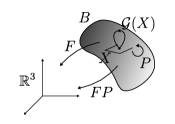
Figure 3. Material symmetry.

Different types of elastic materials are given in terms of their symmetry groups. For instance, a point is solid whenever its symmetry group in some reference configuration is a subgroup of the orthogonal group $O(3)$ and, fluid whenever the orthogonal group is a proper subgroup of the symmetry group. In [7, 14] it is possible to find a classification, due to Lie, of the connected Lie subgroups of $\mathrm{Sl}(3)$ and their corresponding Lie algebras.

Definition 4.2.

Given an elastic material $B$, let $X\in B$ and consider its symmetry group $\mathcal{G}(X)$. If there exists a configuration $K$ such that:

1. $\mathcal{G}_{K}(X)$ is a subgroup of the orthogonal group of transformations $O(3)$, then $X$ is said to be an elastic solid point. If furthermore

   1. $\mathcal{G}_{K}(X)=O(3)$, then we call $X$ a fully isotropic elastic solid point;

   2. $\mathcal{G}_{K}(X)$ is a transverse orthogonal group (a group of rotations which fix an axis), then $X$ is said to be a transversely isotropic elastic solid point;

   3. $\mathcal{G}_{K}(X)$ consists only of the identity element, then $X$ will be a triclinic elastic solid point;

2. $\mathcal{G}_{K}(X)$ is a subgroup of the unimodular group of transformations $U(3)$ and has the orthogonal group $O(3)$ as a proper subgroup, then $X$ is said to be an elastic fluid point. If furthermore

   1. $\mathcal{G}_{K}(X)=\mathrm{Sl}(3)$ then we still call $X$ an elastic fluid; and

   2. $\mathcal{G}_{K}(X)$ is a transverse unimodular group (a group of unimodular transformations which fix an axis or a group of unimodular transformations which fix a plane) then we call $X$ an elastic fluid crystal.

The infinitesimal configuration $T_{X}K$ or the induced frame $z=(T_{X}K)^{-1}$ is called an undistorted state of $X$.

This material classification is pointwise. A body is solid if every point is solid.

5. Uniformity and Homogeneity

To define the uniformity of a material, we first have to give a criterion that establishes when two points are made of the same material. To compare their symmetry groups is not sufficient since this is only a qualitative aspect. Indeed, consider two points in a rubber band, one point may be relaxed while another point may be under stress. But we are still able to release the stress on the second point and bring it to the same state as the first one, and then compare their responses.

Definition 5.1.

We say that two points $X,Y\in B$ are materially isomorphic, if there exists a linear isomorphism $P_{XY}:T_{X}B\rightarrow T_{Y}B$ such that

(5.1) $$\sigma(F\cdot P_{XY},X)=\sigma(F,Y),$$

for any deformation $F$ at $Y$. The linear map $P_{XY}$ is called a material isomorphism.

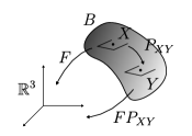
Figure 4. Material isomorphism.

Even if the definition of material isomorphism and material symmetries are mathematically similar, there is an important conceptual difference. While the symmetry group of a point characterizes the material behavior of that point, a material isomorphism establishes a relation between two different points. In fact, as already pointed out, a material symmetry can be viewed as a material automorphism by identifying $X$ with $Y$ in the above definition.

Definition 5.2.

Given a material body $B$, the material groupoid is the set of all the material isomorphisms and symmetries, that is the set

(5.2) $$\mathcal{G}(B)=\left\{P\in\Pi(B)\textrm{ satisfying Definition \ref{def.material.isomorphism}}\right\}.$$

It is easy to check that the material groupoid $\mathcal{G}(B)$ is actually a groupoid. Furthermore, it is a subgroupoid of the frame groupoid $\Pi(B)$, but note that it is not necessarily a Lie groupoid or even transitive as the frame groupoid. In fact, when all the points of a body are pairwise related by a material isomorphism, it means that the body consists only of one type of material. In this case, it is materially uniform.

Definition 5.3.

Given a material body $B$, we say that it is uniform if the material groupoid $\mathcal{G}(B)$ is transitive, and smoothly uniform when the material groupoid is a transitive differential groupoid (and hence a Lie subgroupoid of $\Pi(B)$).

A simple but important property of uniform materials is that the groups of material symmetries are mutually conjugate by any material isomorphism between the respective base points. To be more precise, equation (2.2) reads in terms of elastic bodies:

(5.3) $$\mathcal{G}(Y)=P\cdot\mathcal{G}(X)\cdot P^{-1},\quad\forall P\in\mathcal{G}(B)_{X,Y},$$

for any pair of materially isomorphic points $X,Y\in B$.

When we look a material through different configurations, there are prefered states of the material we want to distinguish: e.g. transversely isotropic solids have a fixed axis “invariant” under material isomorphisms that we prefer to align with the vertical axis. Such a state may be modelized in an infinitesimal configuration by a linear frame $z$. As we have just said, in the material paradigm, this frame of reference $z$ has some behaviors that will be mainted by material isomorphisms. If we consider the set of all these distinguished references that arise from material transformations of the ‘reference crystal’ (see Figure 5), then we obtain the so called material $G$-structure of $B$. As far as we know, Wang was the first to realize that the uniformity of a material can be modelled by a $G$-structure [14], although this fact was emphasized by Bloom [1]. For definiteness,

Definition 5.4.

A material $G$-structure of a smoothly uniform body $B$ is any of the $G_{z}$-structures induced by the material groupoid $\mathcal{G}(B)$ as shown in Theorem 3.5. The chosen frame of reference $z\in\mathcal{F}B$ is called the reference crystal.

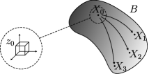
Figure 5. The reference crystal.

Definition 5.5.

Given a smoothly uniform body $B$, a configuration $K$ that induces a cross-section of a material $G$-structure will be called uniform. If there exists an atlas $\left\{(U_{\alpha},K_{\alpha})\right\}_{\alpha\in A}$ of $B$ of local uniform configurations for a fixed material $G$-structure, the body $B$ will be said locally homogeneous, and (globally) homogeneous if the body $B$ may be covered by just one uniform configuration.

The material concept of homogeneity corresponds to the mathematical concept of integrability. By Theorem 3.10, a smoothly uniform body $B$ will be locally homogenous if and only if one (and therefore any) of the associated material $G$-structures is integrable. Let $K$ a uniform configuration for a particular integrable $G$-structure $G(B)$ of a homogeneous elastic material $B$. If $(X,v_{1},v_{2},v_{3})$ denotes the cross section induced by $K$, thus the constitutive equation (4.1) may be written in the form

(5.4) $$\sigma=\sigma(F_{K},K(X))=\sigma(F^{i}_{j},x^{i}),$$

with obvious notation. Now note that, since through $K$ any material isomorphism $P$ may be considered as an element of the structure group $G$, which is clear for material symmetries, and since the body $B$ is uniform, we have that

(5.5) $$\sigma(F^{i}_{j},y^{i})=\sigma(F_{K},K(Y))=\sigma(F_{K}\cdot P_{K},K(X))=\sigma(F^{i}_{k}\cdot P^{k}_{j},x^{i})=\sigma(F^{i}_{j},x^{i}).$$

Thus, we have just proved the following result:

Theorem 5.6.

If $K$ is a uniform configuration of a homogeneous elastic body $B$, the constitutive equation (4.1) is independent of the material point and invariant under the right action of the structure group $G$ of the $G$-structure $G(B)$ related to $K$. Thus,

(5.6) $$\sigma=\sigma(F^{i}_{j})\quad\textrm{and}\quad\sigma(F^{i}_{k}\cdot P^{k}_{j})=\sigma(F^{i}_{j})\ \textrm{for any}\ P\in G.$$

The physical interpretation of this theorem is that points of a homogenous elastic body $B$ can be put by means of a configuration $K$ in such a manner they are all at the same state, at least locally. This configuration $K$ is uniform.

Even if the material $G$-structures of a smoothly uniform body $B$ are different (but equal via conjugation), there must be at least one of them in which the structure group $G$ satisfies a condition of the material classification 4.2.

Definition 5.7.

Accordingly to Definition 4.2, a smoothly uniform elastic body $B$ is solid or fluid, if all the points are solid or fluid, respectively. Any of the material $G$-structures for which the structure group fulfills the classification is called undistorted.

5.1. Uniform Elastic Solids

The following result is due to Wang (cf. [14]). In his paper, Wang defines the material $G$-structures from the point of view of atlases, families of cross-sections of the frame bundle, instead of our approach through groupoids. These families are the cross-sections of the resulting $G$-structures. When a material is solid, it is possible to endow the body with a metric wich is compatible with the material structure. Wang calls such a metric an intrinsic metric.

Theorem 5.8.

Let $B$ be a uniform elastic solid material; each undistorted material $G$-structure $G(M)$ defines a Riemannian metric $g$, invariant under material symmetries and isomorphisms.

Proof.

Given a cross-section $(U,\sigma)$ of a fixed undistorted material $G$-structure $G(B)$, let $X\in U$ and define

(5.7) $$g_{X}^{\sigma}(v,w):=\left\langle\sigma(X)^{-1}\cdot v,\sigma(X)^{-1}\cdot w\right\rangle,\quad\forall X\in U,\forall v,w\in T_{X}B,$$

where $\left\langle\,,\right\rangle$ is the Euclidean scalar product. Thus, $g^{\sigma}$ is clearly a smoooth positive definite symmetric bilinear tensor field on $U$, since it is nothing more than the pullback of the Euclidean metric. Let us check that, in this manner, the metric $g^{\sigma}$ does not depend on the chosen cross-section $(U,\sigma)$. Given any other cross-section $(V,\tau)$, let $X\in B$ be in the intersection of their domains (if not empty, of course), then

(5.8) $$\begin{array}[]{rcl}g_{X}^{\sigma}(v,w)&=&\left\langle\sigma(X)^{-1}\cdot v,\sigma(X)^{-1}\cdot w\right\rangle\\ &=&\left\langle Q\cdot\tau(X)^{-1}\cdot v,Q\cdot\tau(X)^{-1}\cdot w\right\rangle\\ &=&\left\langle\tau(X)^{-1}\cdot v,\tau(X)^{-1}\cdot w\right\rangle\\ &=&g_{X}^{\tau}(v,w),\end{array}$$

where we used the fact that, by hypothesis, $Q=\sigma(X)^{-1}\cdot\tau(X)\in G$ is orthogonal.

Now, let $P\in\mathcal{G}_{X,Y}(B)$ be a material isomorphism; there will exist cross-sections $(U,\sigma),(V,\tau)$ such that $P=\tau(Y)\cdot\sigma(X)^{-1}$. Then, we have

(5.9) $$\begin{array}[]{rcl}g_{Y}(P\cdot v,P\cdot w)&=&\left\langle\tau(Y)^{-1}\cdot P\cdot v,\tau(Y)^{-1}\cdot P\cdot w\right\rangle\\ &=&\left\langle\sigma(X)^{-1}\cdot v,\sigma(X)^{-1}\cdot w\right\rangle\\ &=&g_{Y}(v,w).\end{array}$$

The metric we where looking for is just the metric $g$ defined in (5.7). ∎

If we consider the orthogonal groupoid $\mathcal{O}(B)$ related to this metric, we have that the material groupoid is included in it, $\mathcal{G}(B)\subset\mathcal{O}(B)$. Reciprocally, if $B$ is a smoothly uniform material such that it can be endowed with a Riemannian metric for which the material symmetries and isomorphisms are orthogonal transformations, $\mathcal{G}(B)\subset\mathcal{O}(B)$, then $B$ must be an elastic solid. Thus, elastic solids are completely characterized by Riemannian metrics with the property of being invariant under material symmetries and isomorphisms.

Remark 5.9.

Given two material $G$-structures, $G_{1}(B)$ and $G_{2}(B)$, of a uniform elastic solid $B$, we know that they must be related by the right action of a linear isomorphism $F\in\mathrm{Gl}(3)$, that is $G_{2}(B)=G_{1}(B)\cdot F$. Thus, if $G_{1}(B)$ is undistorted, the $G$-structure $G_{2}(B)$ will be undistorted if and only if the symmetric part $V$ of the left polar decomposition of $F$, $F=V\cdot R$, lies in the centralizer of $G_{1}$, that is $V\in C(G_{1})$ (cf. [14], proposition 11.3). But this does not imply that $G_{1}(B)$ and $G_{2}(B)$ define the same metric, which is true only if $V=I$.

5.2. Uniform Elastic Fluids

There are similar results for fluids as for solids. In this case, the fluid structure induces volume forms.

Proposition 5.10.

Let $B$ be a uniform fluid material, then each undistorted material $G$-structure $G(B)$ defines a volume form $\rho$ invariant under material symmetries and isomorphisms.

Proof.

Given a cross-section $(U,\sigma)$ of a fixed undistorted material $G$-structure $G(B)$, let us define on $U$ the volume form

(5.10) $$\rho_{\sigma}=\sigma^{*1}\wedge\sigma^{*2}\wedge\sigma^{*3},$$

where $\sigma^{*}$ denotes the co-frame cross-section of $\sigma$, that is $\sigma^{*}:U\longrightarrow\mathcal{F}^{*}B$ such that $\sigma^{*i}(\sigma_{j})\equiv\delta^{i}_{j}$ on $U$. Let us show that the volume form $\rho_{\sigma}$ does not depend on the chosen cross-section $(U,\sigma)$. In fact, let $(U,\sigma),(V,\tau)$ be two cross-sections with non-empty domain intersection, then for any $n$ vectors $v_{1},\dots,v_{n}\in T_{X}B$, with $X\in U\cap V$, we have

$$\rho_{\sigma}(v_{1},\dots,v_{n}) = \det(v_{i}^{j})$$

$$= \det((\sigma^{-1}\tau)_{i}^{k})\cdot\det(\tilde{v}_{k}^{j})$$

$$= \rho_{\tau}(v_{1},\dots,v_{n}),$$

where we have used $v_{i}=v_{i}^{j}\sigma_{i}=\tilde{v}_{i}^{j}\tau_{i}$, $v_{i}^{j}=(\sigma^{-1}\tau)_{i}^{k}\cdot\tilde{v}_{k}^{j}$ and $\sigma^{-1}\tau\in U(n)$. Since the tangent vectors $v_{1},\dots,v_{n}$ are arbitrary, $\rho_{\sigma}$ and $\rho_{\tau}$ coincide on the intersection of their domains, $U\cap V$. Thus, the volume form given in (5.10) defines locally a volume form $\rho$ on the whole material body $B$.

Let us see how $\rho$ is invariant under material symmetries and isomorphisms. Given $P\in\mathcal{G}_{X,Y}(B)$, there must exist cross-sections $(U,\sigma),(V,\tau)$ such that $P=\tau(Y)\cdot\sigma(X)^{-1}$. Then, we have

(5.11) $$\rho\circ P=(P^{-1}\tau)^{*1}\wedge(P^{-1}\tau)^{*2}\wedge(P^{-1}\tau)^{*3}=\sigma^{*1}\wedge\sigma^{*2}\wedge\sigma^{*3}=\rho,$$

which finishes the proof. ∎

Considering now the induced unimodular groupoid $\mathcal{U}(B)$, by the invariance we have the inclusion $\mathcal{G}(B)\subset\mathcal{U}(B)$ which also characterizes elastic fluids.

6. Unisymmetry and Homosymmetry

As we have seen, the concept of homogeneity must be understood within the framework of uniformity. But, there are materials that are not uniform by their very definition, the so called functionally graded materials, or FGM for short. This type of material can be made by techniques that accomplish a gradual variation of material properties from point to point: for instance, ceramic-metal composites, used in aeronautics, consist of a plate made of ceramic on one side that continuously change to some metal at the opposite face. The material properties are also given through a constitutive equation like (4.3). Therefore, we will have a notion of material symmetry and the symmetry groups will be non-empty as in the case of uniform materials. For a FGM material, the symmetry groups at two different points are still conjugate, accordingly to the following definition.

Definition 6.1.

Given a functionally graded material $B$, let be $X,Y\in B$; we say that a linear map $A:T_{X}B\longrightarrow T_{Y}B$ is a unisymmetric (material) isomorphism if it conjugates the symmetry groups of $X$ and $Y$, namely,

(6.1) $$\mathcal{G}(Y)=A\cdot\mathcal{G}(X)\cdot A^{-1}.$$

As for uniform bodies, the material properties of a FGM are now characterized by the collection of all the possible unisymmetric isomorphisms.

Definition 6.2.

Given a functionally graded material $B$, the set of unisymmetric isomorphisms, that is the set

(6.2) $$\mathcal{N}(B)=\left\{A\in\Pi(B)\ :\ \mathcal{G}(Y)=A\cdot\mathcal{G}(X)\cdot A^{-1}\right\},$$

will be called the FGM material groupoid of $B$.

Figure 6. The FGM material groupoid.

We may now extend the ideas of section §5 using this new object. Then we obtain:

Definition 6.3.

A functionally graded material $B$ will be said unisymmetric if the FGM material groupoid $\mathcal{N}(B)$ is transitive and, smoothly unisymmetric if it is a Lie groupoid.

Note that the notion of unisymmetry covers a qualitative aspect in the sense that a unisymmetric FGM is made of only one “type” of material. For instance, it will be a fully isotropic solid everywhere or a fluid everywhere, but it cannot be a fully iscotropic solid at some point and a fluid at another point.

For this groupoid, we also have the associated $G$-structures.

Definition 6.4.

Let $B$ be a smoothly unisymmetric body. Any of the asociated $G$-strutures $\mathcal{N}_{z}(B)$, with $z\in\mathcal{F}B$, will be called a material $N$-structure. A cross-section of a material $N$-structure will be a unisymmetric cross-section and a configuration inducing such a cross-section will be a unisymmetric configuration. If for any of the material $N$-structures there exists a covering by unisymmetric configurations, the body $B$ will be said locally homosymmetric, and (globally) homosymmetric if the covering consists of only one unisymmetric configuration.

As we may see, the homosymmetry property is equivalent to the integrability of any of the material $N$-structures. However, there is not an analogue result to Theorem 5.6 for homosymmetric bodies. Since, even if we have an $N$-structure and the group structure is the same for any point through any unisymmetric configuration, the symmetry groups may be represented by different subgroups of $N$ at each point.

6.1. Functionally Graded Elastic Solids

Definition 6.5.

We will say that a functionally graded elastic material $B$ is a functionally graded solid if there is a Riemmanian metric on $B$ invariant under material symmetries, that is every point is solid. Furthermore, $B$ will be said

1. fully isotropic if every point is fully isotropic;

2. transversely isotropic if every point is transversely isotropic; and

3. triclinic if every point is triclinic.

The compatible metric is called a material metric.

We have not used the term “intrinsic” for the material metric, since it does not arise from the material structure as for uniform elastic solids (cf. Theorem 5.8). The material metric is an extra structures that ensures that the solid points are glued in a solid way.

If $B$ is a FGM solid and we consider the orthonormal cross-sections $(U,\sigma)$ of the $O(3)$-structure given by a solid metric, then they must verify:

(6.3) $$\sigma(X)^{-1}\cdot\mathcal{G}(X)\cdot\sigma(X)\subseteq O(3)\quad\forall X\in U\quad\forall(U,\sigma),$$

(6.4) $$\sigma(X)^{-1}\cdot\tau(X)\in O(3)\quad\forall X\in U\cap V\quad\forall(U,\sigma),(V,\tau);$$

where $\mathcal{G}(X)$ is the material symmetry group of $B$ at $X$. In fact, these two conditions are necessary and sufficient to define a solid metric compatible with the material structure by means of a family of cross-sections of $\mathcal{F}B$.

On the other hand, if we consider another $O(3)$-structure, giving a second solid metric, the two structures are not a priori related by the right action of a linear isomorphism $F\in\mathrm{Gl}(3)$. But if they are, then the symmetric part of the polar decomposition of $F$ must be spherical, a homothety. This can be interpreted as the material being in both cases in the same state but the measures of stress, or strain, are performed with different scales.

Definition 6.6.

A solid FGM $B$ will be said to be relaxable if the $O(3)$-structure given by some solid metric is integrable or, equivalently, if the Riemannian curvature (with respect to this metric) vanishes identically. We then say that the $O(3)$-structure is relaxed.

Definition 6.7.

We say that a body $B$ is homosymmetrically relaxable if $B$ is an unisymmetric solid material for which there exists a covering $\Sigma$ of local configuration that are both, unisymmetric and relaxed configurations.

Let $B$ be a homosymmetrically relaxable elastic solid, then we have these two structures, the unisymmetric and the orthogonal, which are in certain manner interconnected. As $B$ is a solid, intuitively we may perceive that only the orthogonal part of a unisymmetric isomorphism must be important. In what follows, we will explain this fact in more detail.

A direct consequence of the previous Lemma 2.11 and Proposition 3.11 is the following theorem, which implies a result proved by Epstein and de León [3].

Theorem 6.8.

If $B$ is relaxable elastic solid that is also homosymmetric, we have

(6.5) $$\bar{\mathcal{N}}(B)=\mathcal{N}(B)\cap\mathcal{O}(B),$$

where $\bar{\mathcal{N}}(B)$ consits in the orthogonal part of the isomorphisms of $\mathcal{N}(B)$. Therefore, if $\bar{\mathcal{N}}_{z}(B)$ is a smooth $\bar{N}_{z}$-structure, $B$ will be homosymmetrically relaxable if and only if the reduced material groupoid $\bar{\mathcal{N}}_{z}(B)$ is integrable (where $z\in\mathcal{F}B$ is fixed).

Let $B$ a relaxable and homosymmetric elastic solid and let $g$ denote the compatible material metric

• If $B$ is fully isotropic, which means the symmetry group $\mathcal{G}(X)$ of each point $X\in B$ is equal to the orthogonal group $O(T_{X}B,g)$ itself, then the reduced FGM material groupoid $\bar{\mathcal{N}}(B)$ coincides with the orthogonal grupoid $\mathcal{O}(B)$.

• If $B$ is triclinic (the only element of the symmetry group is the identity map), the FGM material groupoid $\mathcal{N}(B)$ is the full frame groupoid $\Pi(B)$, and thus $\bar{\mathcal{N}}(B)=\mathcal{O}(B)$ as before.

• If $B$ is transversally isotropic, at each point $X\in B$ there exists a basis of $T_{X}B$ in which the material symmetries $g\in\mathcal{G}(X)$ may be represented by matrices of the form:

  $$\left(\begin{matrix}1&0&0\\ 0&\cos\theta&-\sin\theta\\ 0&\sin\theta&\cos\theta\end{matrix}\right)$$

  Thus, for this basis, the normalizer of $\mathcal{G}(X)$ is

  $$\mathcal{N}(X)=\left\langle\left(\begin{matrix}1&0&0\\ 0&\cos\theta&-\sin\theta\\ 0&\sin\theta&\cos\theta\end{matrix}\right),\left(\begin{matrix}\alpha&0&0\\ 0&\beta&0\\ 0&0&\beta\end{matrix}\right)\right\rangle$$

  where the brackets denote the group generated by the elements enclosed, and where $\theta,\alpha,\beta$ are real numbers, $\alpha,\beta$ being in addition positive. Therefore, the group at any base point of the reduced FGM material groupoid coincides with the respective symmetry group, that is

  $$\bar{\mathcal{N}}(X)=\mathcal{G}(X)\quad\forall x\in B.$$

  This means that, even if the material groupoid $\mathcal{G}(B)$ (the set consisting of material isomorphisms and symmetries) is not transitive (i.e. $B$ is not uniform), the reduced FGM material groupoid $\bar{\mathcal{N}}(B)$ is, and it coincides with $\mathcal{G}(B)$ on the symmetry groups. Thus, there is some kind of uniformity that generalizes the classical one. Finally, note that any $G$-structure related to $\bar{\mathcal{N}}(B)$ will have a transversely isotropic structural group as mentioned before.

  Finally, note that we recover an analogue result to Theorem 5.6, which is also true for fully isotropic FGM solids. If $B$ is homosymmetrically relaxable, then for a unisymmetric and relaxable configuration $K$, the constitutive equation will be invariant under the action of the structure group of the reduced $N$-stucture, related to the configuration $K$. In this case, the structure group will coincide through $K$ with the symmetry group $\mathcal{G}_{K}(X)$ at any point $X$ in the domain of $K$. However, the constitutive equation will not be independent of the point.

6.2. Functionally Graded Elastic Fluids

In the same way we have generalized the definition of elastic solids in section §6.1, we are going to give a new definition of elastic fluids. Classically, an elastic fluid is a uniform elastic material which posses a unimodular material structure, that is a $U(3)$-structure (see [12] for instance), even though there are smaller fluid structures as the ones of fluid crystals (cf. [7]).

Definition 6.9.

We will say that a functionally graded elastic material $B$ is a functionally graded fluid (or a functionally graded fluid crystal) if there is a volume form $\rho$ on $B$ invariant under material symmetries such that every point is fluid (or, respectivelly, if every point is a fluid crystal). The volume form is called a material form.

As in the case of functionally graded elastic solids, the following two conditions on cross-sections $(U,\sigma)$ of the frame bundle $\mathcal{F}B$,

(6.6) $$\sigma(X)^{-1}\cdot\mathcal{G}_{x}\cdot\sigma(X)\subseteq U(3)\quad\forall X\in U\quad\forall(U,\sigma)$$

(6.7) $$\sigma(X)^{-1}\cdot\tau(X)\in U(3)\quad\forall X\in U\cap V\quad\forall(U,\sigma),(V,\tau)$$

characterize the fluid material structure.

Given a functionally graded elastic fluid $B$, consider the unimodular groupoid $\mathcal{U}(B)$ related to the volume form $\rho$ (Example 2.7). When two fluid points have conjugate symmetry groups, only the unimodular part of the conjugate transformation plays a role in the conjugation. That is, if $P$ is the transformation that conjugates these two groups, then the unimodular transformation $P/{\det}_{\rho}(P)$ still realizes the conjugation.

Proposition 6.10.

If $B$ is a unisymmetric elastic fluid, then

(6.8) $$\mathcal{N}^{1}(B)=\mathcal{N}(B)\cap\mathcal{U}(B),$$

where $\mathcal{N}^{1}(B)$ is the unimodular reduction of the FGM material groupoid.

Let $B$ a fluid crystal of first kind (see [7, 14]), that is, an elastic fluid as in 6.9 such that, for each material point $X\in B$, the symmetry group $\mathcal{G}(X)$ may be represented for some reference $z$ at $X$ by matrices of the form

$$A=\left(\begin{matrix}a&b&0\\ c&d&0\\ e&f&g\end{matrix}\right)$$

with $\det(A)=\pm 1$. The normalizer in $\mathrm{Gl}(3)$ of this group of matrices is the set of matrices of the same form but with the restriction $\det(A)\neq 0$. Therefore, when we intersect the normalizer with $U(3)$ we obtain the original group of matrices. This means that $\mathcal{N}^{1}(X)=\mathcal{G}(X)$ for every material point $x\in B$.

The latter example shows us how a fluid material, which is not necessarilly uniform, preserves uniformly the symmetry group structure across the body.

References

- [1] F. Bloom, Modern differential geometric techniques in the theory of continuous distributions of dislocations, Lecture Notes in Math. 733, Springer, Berlin, 1979.
- [2] M. Elżanowski, M. Epstein, J. Śniatycki, -structures and material homogeneity, J. Elasticity 23 (no. 2-3) (1990), 167–180.
- [3] M. Epstein, M. de León, Homogeneity without uniformity: towards a mathematical theory of functionally graded materials, Internat. J. Solids Structures 37 (no. 51) (2000), 7577–7591.
- [4] A. Fujimoto, Theory of -structures, Study Group of Geometry, Department of Applied Mathematics, College of Liberal Arts and Science, Okayama University, Okayama, 1972.
- [5] S. Kobayashi, K. Nomizu, Foundations of differential geometry. Vol. I, John Wiley & Sons Inc., New York, 1996.
- [6] by same author, Foundations of differential geometry. Vol. II, John Wiley & Sons Inc., New York, 1996.
- [7] M. de León, D. Marín, Classification of material -structures, Mediterr. J. Math. 1 (no. 4) (2004), 375–416.
- [8] K. Mackenzie, Lie groupoids and Lie algebroids in differential geometry, London Mathematical Society Lecture Note Series, vol. 124, Cambridge University Press, Cambridge, 1987.
- [9] J. Marsden and T. Hughes, Mathematical foundations of elasticity, Dover Publications Inc., New York, 1994.
- [10] W. Noll, Materially uniform simple bodies with inhomogeneities, Arch. Rational Mech. Anal. 27 (1967/1968), 1–32.
- [11] C. Truesdell, A first course in rational continuum mechanics. Vol. 1, Academic Press, New York, 1977.
- [12] C. Truesdell and W. Noll, The nonlinear field theories of mechanics (second ed.), Springer-Verlag, Berlin, 1992.
- [13] C. Truesdell and C. C. Wang, Introduction to rational elasticity, Noordhoff International Publishing, Leyden, 1973.
- [14] C.-C. Wang, On the geometric structures of simple bodies. A mathematical foundation for the theory of continuous distributions of dislocations, Arch. Rational Mech. Anal. 27 (1967/1968), 33–94.