Spectra of graphs and semi-conducting polymers

Abstract.

We study the band gap in some semi-conducting polymers with two models: Hückel molecular orbital theory and the so-called free electron model. The two models are directly related to spectral theory on combinatorial and metric graphs. Our numerical results reproduce qualitatively experimental results and results from much more complex density-functional calculations. We show that several trends can be predicted from simple graph models as the size of the object tends to infinity.

1. Introduction

An important pattern in organic chemistry are delocalized electron systems, also called conjugated $\pi$-electron systems. Most dyes owe their color to such structures. When the length of a conjugated electron system becomes large, electric conductivity and luminescence are possible.
This is achieved in practice by chemically connecting a fragment with delocalized electrons to its copy, and repeating this procedure many times. The original fragment is called monomer; if the number of copies is definite and rather small (up to few tenths), the resulting product is called oligomer; if the number of segments is large and indefinite, the resulting product is called polymer. Semi-conducting polymers are the basis for organic light-emitting diodes (LED’s) and transistors [5]; oligomers can be used in photovoltaic devices [33].

An important open question about these chemical structures is whether and how it is possible to extrapolate the electronic structure of oligomers with increasing number $m$ of segments to that of the polymer. The asymptotics of the band gap $\triangle E(m)$ of oligomers with length $m$ increasing to infinity is subject to ongoing debate [4, 7, 17, 27, 28, 32, 43]. It is known both from experiments and quantum chemical calculations that the convergence behavior of the band gap of oligomers with increasing length to the band gap of the polymer often deviates from $\triangle E(m)-\triangle E(\infty)\propto 1/m$. One might expect the latter relation based on the behavior of a linear chain of length $m$ in the limit $m\rightarrow\infty$. The latter can be calculated straightforwardly and has been observed experimentally [2] (the finite chain corresponds to a C_2mH_2m+2 poly-acetylene oligomer, PA$m$).

(a) Benzene

(b) Naphthalene

      

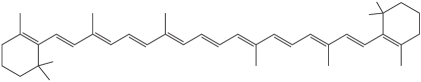
(c) $\beta$-carotene

Figure 1. Molecules with conjugated $\pi$-systems. Carbon atoms are conventionally points connected by bonds. Hydrogen atoms are not displayed.

We will use the following notation for oligomer/polymer molecules: the polymer is abbreviated by 2-5 letters related to its full name, e.g. PA (poly-acetylene), PPP (poly-para-phenylene). A number $m$ following this abbreviation refers to an oligomer with $m$ copies of the corresponding monomer, e.g. PPP$5$ is the para-phenylene oligomer C₃₀H₃₀. It consists of 5 connected copies of the C₆H₆ monomer benzene.

In this paper we discuss the gap $\triangle E(m)$ and its convergence in the polymer limit ($m\to\infty$)for quantum chemical models that reduce to solving an eigenvalue problem on either combinatorial or metric graphs. Some background on these models will be given in Section 2. In Section 3 we will define the spectral problems on graphs and describe how they are related to oligomers. We will also explicitly solve the simplest polymer (poly-acetylene in either ring or chain formation) as an example in Section 3.1 and summarize the (well-known) Floquet-Bloch theory for the infinite polymer in Section 3.2. Eventually we will present and discuss numerical results for a number of relevant polymers in Section 4 and compare those to experimental data.

(a) PA

(b) PPP

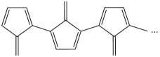
(c) PPf

Figure 2. Conjugated polymers poly-acetylene, poly-para-phenylene, poly-pentafulvene.

2. Conjugated double bonds: beyond valence bond theory

Conventionally, organic molecules are described by covalent bonds. According to the valence-bond (VB) theory the outer shell (valence) electrons spatially rearrange themselves such that a pair of electrons is shared by two atoms while inner shell electrons remain assigned to individual atoms of the molecule. A single covalent bond consists of one pair of electrons. Double and triple bonds between two atoms consist correspondingly of two or three pairs of electrons shared between the atoms. Recall that one single carbon atom has four valence electrons and it forms hence four bonds. Some of these may constitute a double or triple bond. A sequence of alternating single- and double C–C bonds is called conjugated, see Fig. 1 for examples.

The VB assumption fails to explain the properties of compounds with conjugated sequences already on a qualitative level. Absorption spectra, luminescence and conductivity indicate that the spacing between energy levels in such molecules is much lower than in similar non-conjugated counterparts. This strongly indicates that some electrons in these molecules are delocalized over a much larger region than one single or double bond, in contrast to the VB theory.

The more general Molecular Orbital (MO) Theory overcomes the shortcomings of the VB theory [40]. It postulates that valence electrons recombine and form molecular orbitals to minimize the total energy of the entire molecule. The following two models have been put forward to describe conjugated systems in the framework of MO Theory. Both neglect the repulsion and correlation of electrons. Erich Hückel suggested the following scheme for molecules with alternating double bonds [13, 14, 15, 16]:

• Single covalent bonds between adjacent atoms are formed and they determine the geometry of the molecule.

• The remaining electrons (also called $\pi$-electrons, in a conjugated system there is one $\pi$-electron per carbon atom) and their wave functions are subject to energy minimization. This reduces to an eigenvalue problem on a combinatorial graph after some further simplifying assumptions. This spectral problem is referred to as the Hückel Molecular Orbital (HMO) Theory.

The alternative to the HMO approach is based on the assumption that the electrons of a conjugated system are strongly bound to the positively charged carbon-backbone [38], which is modeled as a graph [26, 37]. Interestingly, in the original formulation Hans Kuhn already considered atoms as scattering centers for the electron wave functions. This is the Free Electron Model (FE). This model can be reduced (after separation of variables) to an eigenvalue problem on a metric graph for the Schrödinger operator without a potential (hence the ‘free electron’ in the name). The assumptions of this model are only plausible for large systems.

For finite molecules both, the MO and the FE model, yield discrete energy levels $E_{n}$ with corresponding eigenfunctions (molecular orbitals). Owing to spin, each of these levels can be occupied by two electrons (applying Hund’s rule and the Pauli exclusion principle). In a system with $M$ alternating double bonds there are $2M$ $\pi$-electrons. In the ground state of the system, the $M$ lowest molecular orbitals are occupied. The energy of the highest occupied molecular orbital (HOMO) is thus $E_{HOMO}=E_{M}$. The energy of the lowest unoccupied molecular orbital (LUMO) is $E_{LUMO}=E_{M+1}$.
The difference $\triangle E=E_{LUMO}-E_{HOMO}$ is the smallest energy package a molecule can absorb. It is directly related to the color of a material (i.e. to the highest absorbed wave length) and to the breakdown voltage of semi-conducting materials (since this is proportional to the band-gap). In Ref. [42] band gaps of several semi-conductive polymers have been studied qualitatively using HMO theory.

The degeneracy of $E_{M}$ can determine chemical properties of a compound. If $E_{M}$ is a multiple, completely occupied energy level, then the compound is chemically stable and inert. The classical example is nitrogen. Conversely, if $E_{M}$ is multiple and not completely occupied (SOMO, where “S” stands for “singly”), then the compound is chemically reactive. The classical example is oxygen. The existence of such orbitals in conjugated hydrocarbons is related to the question whether 0 is an eigenvalue of the adjacency matrix of the underlying graph, see [3, Chapter 8] which is dedicated to this topic.

One advantage of the HMO theory is that absolute energy levels can be calculated. As a consequence it is possible to investigate the stability of compounds. Moreover, the underlying MO theory is not restricted to conjugated systems.
On the other side, the FE model has the advantage that no parameter fitting is involved. Moreover, wave functions and electron densities can easier be calculated in the FE model. The latter information can then be used to infer statements about bond lengths and effect of heteroatoms [25].

3. Mathematical description of polymers by combinatorial and metric graph models

For a given molecule with a conjugated fragment and $N_{C}$ carbon atoms, it is straightforward to define the underlying graph $G$. The vertices $v_{i}$ (where $i=1,2,\dots,N_{C}$) of the graph are the carbon atoms and the undirected bonds $b$ of the graph are the chemical bonds between them. For the undirected bond connecting the vertices $v_{i}$ and $v_{j}$ we write $b_{ij}\equiv b_{ji}$. Note that on the graph $G$ all bonds are simple, disregarding their chemical multiplicity. We write $i\sim j$ if the vertices (atoms) $v_{i}$ and $v_{j}$ are connected. The undirected (metric) graph is fully characterized by its $N_{C}\times N_{C}$ symmetrical bond matrix $B$, where $B_{i,j}=B_{j,i}$ is the bond length between the two carbon atoms (vertices) $v_{i}$ and $v_{j}$ if they are connected, and $0$ otherwise. In the following all bonds in a purely hydrocarbon system are assumed identical, unless the opposite is stated. By replacing all bond lengths in $B$ with unity one obtains the $N_{C}\times N_{C}$ connectivity matrix $C$.

HMO theory in its original formulation solves the eigenvalue problem

(3.1) $$Cu=\lambda u.$$

Since $C$ is a real symmetric matrix, it has $N_{C}$ real eigenvalues $\lambda_{1},\dots,\lambda_{N_{C}}$. The electronic energy levels $E_{n}$ in a molecule are related to the eigenvalues $\lambda_{n}$ of the connectivity matrix by

(3.2) $$E_{n}=\lambda_{n}\beta-\alpha,\quad n=1,\dots,N_{C}$$

where $\beta$ and $\alpha$ are constant parameters with units of energy. The value of $\alpha$ is not relevant for pure hydrocarbon compounds since it is just a constant shift. The parameter $\beta$ is defined as a resonance integral, but is usually fitted to experimental data. In order to keep results consistent with the FE model, we choose $\beta=3.05$eV as in Ref. [41]. It is important to note that the parameters $\alpha$ and $\beta$ are not potentials in the physical sense, and that the eigenvectors $u_{n}$ are not the values of the wave function at the vertices.

To formulate the FE model, we need to define a real coordinate $0\leq x_{ij}\leq B_{ij}$ along each undirected bond $b_{ij}$. For $i<j$ we set $x_{ij}=0$ at one end of the bond where it is connected to the vertex $v_{i}$ and $x_{ij}=B_{ij}$ at the other end connected to $v_{j}$. We will also use the notation $x_{ij}=v_{i}$ for the value of $x_{ij}$ at vertex $v_{i}$. The metric graph is quantized by defining a self-adjoint Schrödinger operator for a wave function $\Phi(x)$ on the metric graph.
This implies that the wave function $\Phi(x)$ must satisfy the one-electron free Schrödinger equation on each bond $b_{ij}$

(3.3) $$-\frac{\hbar^{2}}{2m_{e}}\frac{d}{dx^{2}_{ij}}\Phi(x_{ij})=E\Phi(x_{ij})$$

with Plank’s constant $\hbar$, electron mass $m_{e}$ and energy $E$.
To obtain a self-adjoint Schrödinger operator one has to add certain conditions on the wave functions at the vertices [9, 18, 19]. We will impose the Neumann conditions (also known as Kirchhoff conditions) that the wave function is continuous at each vertex

(3.4) $$\text{for all $j\sim i$}\;\lim_{x_{ij}\rightarrow v_{i}}\Phi(x_{ij})= \Phi(v_{i})$$

and, additionally that the sum over all outgoing derivatives of the wavefunctions on all bonds connected to a vertex vanishes

(3.5) $$\left.\sum_{j:j\sim i}w_{j}^{i}\frac{d}{dx_{ij}}\Phi(x_{ij})\right|_{x_{ij}=v_{i}}= 0$$

where $w_{j}^{i}=1$ if $i<j$ and $w_{j}^{i}=-1$ otherwise.

Solving the Schrödinger Equation (3.3) with vertex conditions (3.4-3.5) we obtain discrete energy levels $E_{n}$ and wave functions (MOs) $\Phi_{n}$.

Additional potentials on the bonds have been introduced in Eq. (3.3) to improve the agreement with experimental values [26, 37]. One may also add vertex potentials to get a more realistic description (see [9, 19]). Any such generalization adds some fitting parameters. In this work we are mainly interested in more fundamental questions concerning the convergence behavior for general polymers and we thus stick to the simplest model and no fitting parameters.

We scale the bond lengths of the graph to the average C–C bond length of $L_{C-C}=1.4$Å and $\frac{\hbar^{2}}{2m_{e}}$ to $1$. The eigenvalues $\mu_{n}$ of the scaled problem correspond to electronic energy levels as $E_{n}=\mu_{n}\epsilon$ with $\epsilon=\frac{\hbar^{2}}{2m_{e}L_{C-C}^{2}}=1.95$eV.

In order to find the eigenvalues numerically, one has to solve the secular equation (see [9, 19] for details). However, throughout this work we assume equal bond lengths. Then the following identity is valid [34]. Define the diagonal valency matrix $V$ (i.e. $V_{i,i}$ is the number of bonds at the vertex $v_{i}$). If $\mu$ is an eigenvalue of the (scaled) FE problem, then $\tilde{\mu}=\cos\sqrt{\mu}$ is an eigenvalue with the same multiplicity of the generalized eigenvalue problem

(3.6) $$Cu=\tilde{\mu}Vu.$$

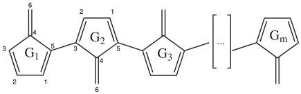
Figure 3. Construction of the oligomer PPf$m$, chemical notation is used to represent the graph. The fifth carbon atom of the first monomer in the chain is connected to the third atom of the second one etc. In the graph notation this means $v_{5}^{1}\sim v_{3}^{2}$; the index $b$ is $5$ and the index $e$ is $3$.

We adopt the following notation for oligomers and polymers, see also Fig. 3. A monomer $X\equiv X1$ is described by a graph that we will call $G_{1}$. The number of carbon atoms in the monomer will be denoted by $N_{C}$ and is equal to the number of vertices in $G_{1}$, and $N$ will be used for the number of double bonds in the monomer. Usually, $N_{C}=2N$. The monomer has two atoms at which bonds to other monomers of the same type are created. Let these atoms be represented by the vertices $v_{b},v_{e}$, so that two consecutive monomers are connected by a bond between the atom $b$ of the first and $e$ of the second monomer. Let us now consider $m$ copies $G_{1},G_{2},G_{3},\dots,G_{m}$ of the monomer $G_{1}$. Denote the vertex $v_{i}$ on $G_{a}$ by $v_{i}^{a}$. We can now construct the graph $G^{m}$ that represents the oligomer $Xm$ as a union $G^{m}=\bigcup_{a=1}^{m}G_{a}$ with extra bonds between $v^{a}_{b}$ and $v^{a+1}_{e},\ a=1,\dots,m-1$. Obviously one has $G_{1}=G^{1}$. The band gap of $G^{m}$ is

(3.7) $$\triangle E(m)=E_{M+1}-E_{M}$$

where $M=Nm$ is the number of double bonds on the oligomer.

The above construction assumes that adjacent monomers are connected via a single bond between two atoms. We only consider polymers of this type here. Note that the construction can easily be generalized to incorporate many bonds between adjacent monomers.

3.1. Examples: rings and chains

Consider a ring C_2mH_2m consisting of $M=m$ alternating double bonds. It has $N_{C}=2$ carbon atoms per ”monomer”, each with $N=1$ (trivially) alternating double bond. The HMO-eigenvalues are

(3.8) $$\lambda_{n}=2\cos(\frac{n\pi}{m}),\quad n=1,2,\dots,2N$$

while the FE eigenvalues are

(3.9) $$\mu_{n}=\frac{n^{2}\pi^{2}}{m^{2}},\quad n=0,\pm 1,\pm 2,\dots$$

We see that both models predict qualitatively the same energy scheme. The ground state is simple, higher states are double (except for $\lambda_{2m}$, which is not important). Thus, $E_{m}$ and $E_{m+1}$ are both double. For odd $m$, $E_{HOMO}$ is completely filled, yielding an increased chemical stability, while for even $m$ it is not complete leading to an increased reactivity. This is the famous Hückel rule.

Consider now a chain C_2mH_2m+2 with $M=m$ alternating double bonds (polyenes). The limit $m\to\infty$ is the most trivial example for a conjugated polymer and is called poly-acetylene (PA). It was the first polymer for which electric conductivity was shown and studied.

The HMO and FE eigenvalues are

(3.10) $$\lambda_{n} =2\cos\left(\frac{n\pi}{2m+1}\right),\quad n=1,2,\dots,2m$$

(3.11) $$\mu_{n} =\frac{n^{2}\pi^{2}}{(2m-1)^{2}},\quad n=0,1,2,\dots$$

respectively . Now all energy levels a single. The HOMO-LUMO difference in HMO is

(3.12) $$\triangle E_{HMO}(m)=E_{m+1}-E_{m}=-4\beta\sin\left(\frac{\pi}{4m+2}\right)$$

and in FE

(3.13) $$\triangle E_{FE}(m)=E_{m+1}-E_{m}=\epsilon\pi^{2}\left(\frac{2m+1}{(2m-1)^{2}}\right).$$

We see that both models predict $\triangle E(\infty)=0$ and $\triangle E(m)-\triangle E(\infty)\propto\frac{1}{m}$ for large $m$. In both models, the discrete electronic levels become one single band in the $m\to\infty$ limit. In practice, the band gap of PA is significant ($1.8$eV), but the convergence behavior $\triangle E(m)-\triangle E(\infty)$ is almost linear in $1/m$ with the slope close to the FE and HMO case, see Section 4.

3.2. Polymer limit

In the limit $m\to\infty$ the underlying graph $G^{\infty}$ is periodic and Floquet-Bloch Theory can be applied [1, 11, 20, 22, 23, 24, 36]. Consider the HMO eigenvalue problem (the FE case is analogous and will not be discussed in detail)

(3.14) $$C_{G^{\infty}}\Psi=\lambda\Psi.$$

All physically relevant eigenvector candidates (bound states) can be found as a product of a periodic function and a phase shift:

(3.15) $$\Psi(v_{i}^{j+1})=e^{ik}\Psi(v_{i}^{j}),$$

where we introduced the quasi-momentum $k\in\left[-\pi,\pi\right]$. For a multiple eigenvalue $\lambda$, Floquet-Bloch eigenfunctions span the eigenspace. The eigenvalue problem on $G^{\infty}$ reduces to the problem on a single monomer

(3.16) $$(C+F(k))\Psi=\lambda(k)\Psi$$

where $F(k)$ is a $N_{C}\times N_{C}$ matrix with only two non-zero entries at the connection between monomers $F_{eb}(k)=e^{ik}$ and $F_{be}(k)=e^{-ik}$. Since $C+F(k)$ is a Hermitian matrix, it has $N_{C}$ real eigenvalues $\lambda_{1}(k),\dots,\lambda_{N_{C}}(k)$. Each of the branches $\lambda_{r}(k)$ is a continuous function of $k$. The set $\bigcup_{0\leq k\leq\pi}\lambda_{r}(k)$ is the $r$th band. The $N$th band is called the valence band while the $(N+1)$th band is the conduction band.

The spectrum of $C_{G^{\infty}}$ is the union of all bands

(3.17) $$\sigma(C_{G^{\infty}})=\bigcup_{0\leq k\leq\pi}\bigcup_{r=1,\dots,2N}\lambda_{r}(k).$$

Due to the one-dimensional periodicity and the fact that the monomers are connected by one single bond, the extrema of $\lambda_{r}(k)$ are always at $k=0$ or $k=\pi$. Consider the characteristic polynomial $\xi$ of $C+F(k)$ as a function of $k$ and $\lambda$

(3.18) $$\xi(k,\lambda)=\det(C+F(k)-\lambda I_{N_{C}})$$

where $I_{N_{C}}$ is the unit matrix. Eigenvalues are given by $\xi(k,\lambda)=0$, and hence the Implicit Function Theorem can be applied: if $\frac{\partial\xi}{\partial\lambda}\neq 0$ in a neighborhood of $\tilde{k},\tilde{\lambda}$ with $\xi(\tilde{k},\tilde{\lambda})=0$, then $\lambda(k)$ is a well-defined, differentiable function in this neighborhood with

(3.19) $$\frac{d\lambda}{dk}=-\left(\frac{\partial\xi}{\partial\lambda}\right)\times\left(\frac{\partial\xi}{\partial k}\right).$$

One easily finds that

(3.20) $$\frac{\partial\xi}{\partial k}=ie^{ik}(-1)^{e+b}M_{e,b}-ie^{-ik}(-1)^{e+b}M_{b,e}=\\ -2\,(-1)^{e+b}{\rm Im}(e^{ik}M_{e,b})={\rm Im}\left[e^{ik}\left(m_{0}(\lambda)+m_{1}(\lambda)e^{-ik}\right)\right]=m_{0}(\lambda)\sin k$$

where $M_{e,b}$ is the $e,b$-minor of $C+F(k)-\lambda I_{N_{C}}$, i.e. the determinant of the matrix after deleting the $e$th row and $b$th column; $m_{0},m_{1}$ are some polynomials in $\lambda$. The first equation follows from the rule for determinant derivatives; the second one from the fact that $M_{e,b}=\overline{M}_{b,e}$; the third one because $M_{e,b}$ has only one entry which depends on $k$; and the last one because $m_{1}(\lambda)$ is real. We obtain therefore

(3.21) $$\xi(k,\lambda) =p_{0}(\lambda)\cos(k)+p_{1}(\lambda), \frac{\partial\xi}{\partial\lambda} =p^{\prime}_{0}(\lambda)\cos(k)+p^{\prime}_{1}(\lambda)$$

with some polynomials $p_{0}$ ($=-m_{0}$) and $p_{1}$. Obviously, $\lambda(k)=\lambda(-k)$ and $\lambda$ determines $k\in[0,\pi]$ uniquely iff $p_{0}$ does not vanish. Now three cases are possible for an eigenvalue $\tilde{\lambda}$:

1. $p_{0}(\tilde{\lambda})=p_{1}(\tilde{\lambda})=0$. Then $\xi(k,\tilde{\lambda})$ does not depend on $k$, and $\tilde{\lambda}$ is a degenerate band $\lambda(k)=\tilde{\lambda}$. And, conversely, if $\tilde{\lambda}$ belongs to a non-degenerate band, then $p_{0}(\tilde{\lambda})\neq 0$.

2. $\frac{\partial\xi}{\partial\lambda}(\tilde{\lambda})=0$. This means that $\tilde{\lambda}$ is a multiple eigenvalue, i.e. belongs to two (or more) bands. In this case, the two bands join. Assume namely, that two non-degenerate bands overlap, i.e. there exists an interval $(\lambda_{-},\lambda_{+})$ of “double” eigenvalues. Then, according to Eq.(3.21), almost everywhere on this interval would hold $\cos(k)=p_{1}(\lambda)/p_{0}(\lambda)$ and $p^{\prime}_{0}(\lambda)p_{1}(\lambda)+p^{\prime}_{1}(\lambda)p_{0}(\lambda)=0$. Therefore, both $p_{0}$ and $p_{1}$ must be constant, which is only possible for empty graphs.

3. Otherwise, $p_{0}(\tilde{\lambda})\neq 0$ on the entire band, and the extrema of $\lambda(k)$ within this band are given by the zeros of Eq.(3.20), i.e. integer multiples of $\pi$.

Thus, in all cases the band edges are contained in the eigenvalues of $C+F(0)$ and $C+F(\pi)$ ($e^{ik}=\pm 1$). Note that in the second case no statement is made for degenerate bands. Remarkably, if $F(k)$ has more than two non-zero entries, i.e. the monomers are connected by more than one bond, then the arguments of Eq.(3.20) become incorrect, and a counterexample to the statement about band edges can be found in [11].

To study and compare spectral bands of oligomers and polymers, it is useful to define for a real number $x$ the spectral counting function as the number of eigenvalues per monomer, which are smaller than $x$. For an oligomer this is given by

(3.22) $$\sigma^{m}(x)=\frac{\{n|\lambda_{n-1}<x\leq\lambda_{n}\}}{m}.$$

where the eigenvalues $\lambda_{0},\lambda_{1},\dots$ are put in increasing order and $\lambda_{-1}\equiv-\infty$. The spectral counting function of the polymer is obtained by taking the limit $m\to\infty$.
Intervals where $\sigma$ increases continuously correspond to bands; intervals where it is constant correspond to band gaps. Jumps are degenerated bands: e.g. if $G_{1}$ has an eigenvalue $\Lambda$ with an eigenstate which vanishes at the vertices $v_{b}$ and $v_{e}$ then the oligomer will have an $m$-fold degenerate eigenvalue with quasi-momentum $k=0$ and $\lambda_{1}(0)=\lambda_{2}(0)=\dots=\lambda_{m}(0)=\Lambda$ with eigenstates which are localized on one monomer. Such eigenstates do not satisfy Eq. (3.15), but lie in the space spanned by Floquet-Bloch eigenfunctions.

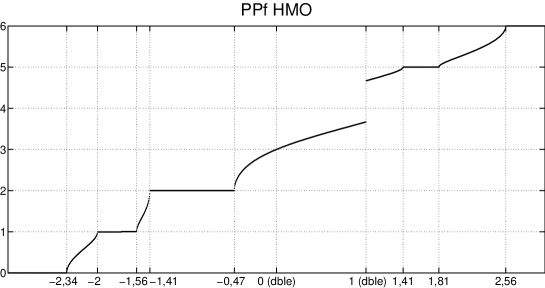
Figure 4. $\sigma^{200}_{\rm HMO}$ and Floquet-Bloch Theory of PPf. The twelve band edges arranged in increasing order $-2.34$, $-2$, $-1.56$, $-1.41$, $-0.47$, $0$, $0$, $1$, $1$, $1.41$, $1.81$, $2.56$ are displayed on the horizontal axis.

Consider PPf, see Fig. 3. The matrices $C$ and $F(k)$ are

(3.35) $$C =\left(\begin{array}[]{cccccc}0&1&0&0&1&0\\ 1&0&1&0&0&0\\ 0&1&0&1&0&0\\ 0&0&1&0&1&1\\ 1&0&0&1&0&0\\ 0&0&0&1&0&0\\ \end{array}\right); F(k) =\left(\begin{array}[]{cccccc}0&0&0&0&0&0\\ 0&0&0&0&0&0\\ 0&0&0&0&e^{ik}&0\\ 0&0&0&0&0&0\\ 0&0&e^{-ik}&0&0&0\\ 0&0&0&0&0&0\\ \end{array}\right).$$

The calculated $\sigma^{200}_{\rm HMO}$ is shown in Fig. 4 together with the band edges from Floquet-Bloch Theory. The first two bands are $[-2.34,-2]$ and $[-1.56,-1.41]$. Since $0$ and $1$ appear twice, there are no gaps between the third, fourth and fifth bands. The last band is then $[1.81,2.56]$. Knowing that $0$ is a double eigenvalue of $C+F(0)$ while $1$ is a simple eigenvalue of $C+F(0)$ and $C+F(\pi)$, we conclude that there is a jump at $1$ and no jump at $0$.

4. Examples and comparison with experiment

It is important to note that experimentally determined band gaps systematically differ from the ones predicted by simple theories. The differences are due to (i) intermolecular phenomena such as electronic repulsion, electron correlation, spatial geometry, non-conjugated side chains and (ii) intermolecular effects such as solvent or solid-state shifts and impurities. These effects are approximately constant ($\approx 1$eV) for a given sequence of oligomers at the same experimental conditions [7]. The band gap of a (real) material is influenced by the environment, therefore different measurements on the same compound may give slightly different values depending on experimental conditions.

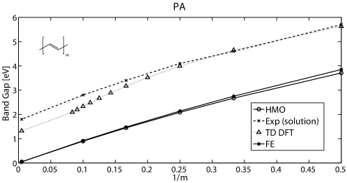
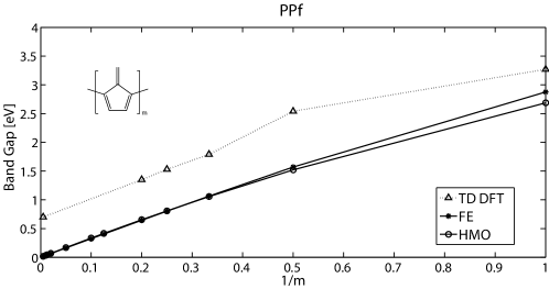
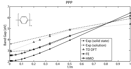
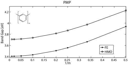
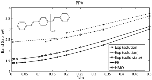
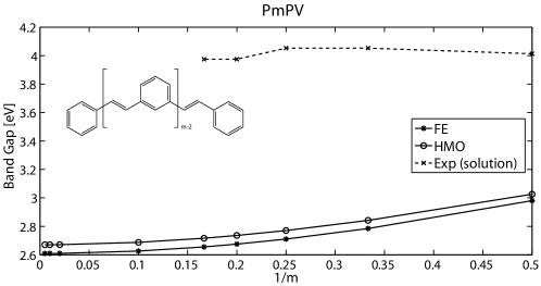
Figure 5. Band gaps of oligomers estimated by HMO and FE models compared with experimental values. On the horizontal axis is the inverse number of monomers. HMO-values are represented by circles; FE-values by stars. Sources: all TD DFT calculations [29]; PA [2]; PPP [30],[31]; PPV [6],[8],[7]; PmPV [10].

We consider the following polymers: PA ($N_{C}=2$, $N=1$), PPf (poly-pentafulvene, $N_{C}=6$, $N=3$), PPP ($N_{C}=6$, $N=3$), PMP (poly-meta-phenylene, $N_{C}=6$, $N=3$), PPV (poly-phenylene-vinylene, $N_{C}=8$, $N=4$) and PmPV (poly-meta-phenylene-vinylene, $N_{C}=8$, $N=4$), see also Fig. 2. The first one is the alternating chain and has already been discussed in Section 3.1. The second one, PPf represents the large number of $5$-ring based polymers. To the best of our knowledge, it is subject to theoretical studies [12, 35] as a possible low-band-gap polymer, but has not been synthesized yet. The other four are based on benzene (6-ring) as monomer but connected differently. PMP has a $1-3$ connection (meta) whereas PPP has a $1-4$ connection (para). PPV and PmPV have additionally two carbon atoms between the rings, i.e. the connection length is $3$ and $N=4$. Note that PPP$2$=PMP$2$ and PPV$2$=PmPV$2$.

As we can see from Fig. 5, both models predict similar trends and values. The estimated band gaps are mostly within 1eV below the experimental values. PPf is the only polymer showing a PA-like behavior: the band gap converging to $0$ as $1/m$. This can be explained by symmetry arguments [42]. The non-linear (in $1/m$) convergence of other oligomer series is in line with experimental observations. The band gap decreases by $1.5-2$eV between $m=2$ and $m=\infty$ in series of para-connected oligomers PPP$m$ and PPV$m$, whereas for the meta-connected PMP$m$ and PmPV$m$ this decrease is only $\approx 0.5$eV, in a good agreement with available experimental data. We have also compared our results with Time Dependent Density Functional Theory (TD DFT) calculation [29], data represented by triangles. These data compare better with measurements than the FE or HMO predictions, but provide less information about trends.

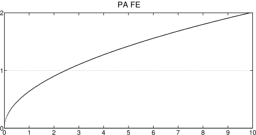
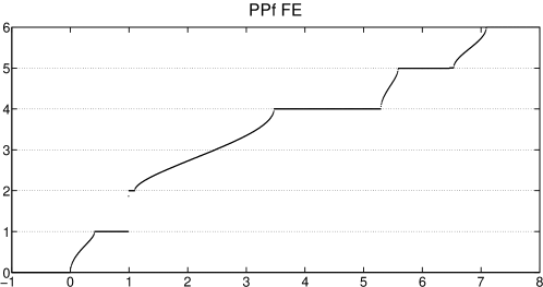
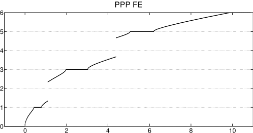
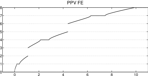
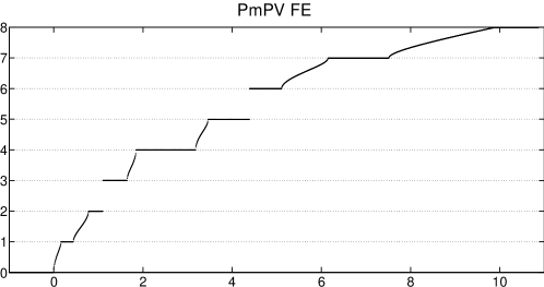
Figure 6. Spectral counting function $\sigma^{200}_{\rm FE}$ of PA, PPf, PPP, PMP, PPV and PmPV in the FE model

Another crucial property for conductivity is the width of the valence and conduction bands. We have calculated $\sigma^{m}_{\rm HMO}$ and $\sigma^{m}_{\rm FE}$ for the six above polymers ($m=200$) in Figs. 6 and 7.

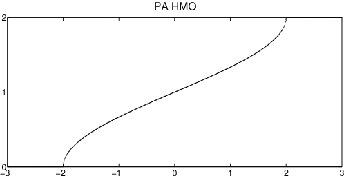
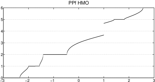
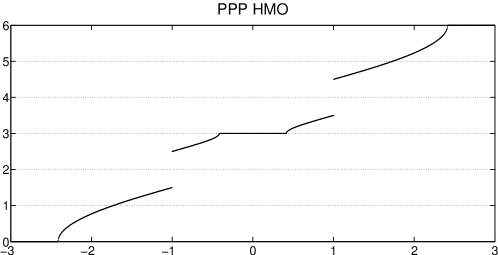
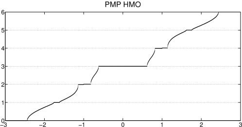
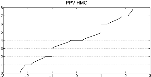
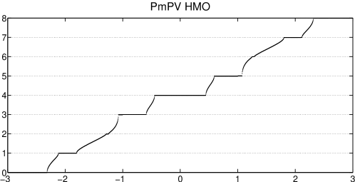
Figure 7. Spectral counting function $\sigma^{200}_{\rm HMO}$ of PA, PPf, PPP, PMP, PPV and PmPV in the HMO model

As discussed above, the band gaps of PA and PPf vanish. We can see that the para-connected polymers have much wider valence and conduction bands than their meta-connected counterparts. Together with the smaller band gaps this explains why PPP and PPV are good conductors while PMP and PmPV are not [39].

5. Conclusions

We have studied conducting polymers from the point of view of Hückel Molecular Orbital Theory and Free Electron Model, the two models directly related to the spectral graph theory. Qualitative predictions match the experimental reality. Floquet-Bloch theory for periodic graphs provides means for an easy study of band properties of polymers.

Quantitative comparison shows that actual band gaps can be reasonably estimated by either of the models when correcting for intramolecular and intermolecular shifts. The absence of any parameter fitting makes this result particularly exciting. The convergence behavior $\triangle E(m)-\triangle E(\infty)$ of band gaps of oligomer series is well reproduced. Therefore, it is possible to extract the band gap of the polymer from the data for finite values of $m$ with sufficient accuracy using simple graph models. It would be promising for practical applications to derive an analytic expression for $\triangle E(m)$.

References

- [1] J. E. Avron, P. Exner, and Y. Last. Periodic Schrödinger operators with large gaps and Wannier-Stark ladders. Physical Review Letters, 72(6):896–899, 1994.
- [2] J. L. Brédas, R. Silbey, D. S. Boudreaux, and R. R. Chance. Chain-length dependence of electronic and electrochemical properties of conjugated systems: Polyacetylene, polyphenylene, polythiophene, and polypyrrole. Journal of the American Chemical Society, 105(22):6555–6559, 1983.
- [3] Dragoš M. Cvetković, Michael Doob, and Horst Sachs. Spectra of graphs. Johann Ambrosius Barth, Heidelberg, third edition, 1995. Theory and applications.
- [4] S. Dähne and R. Radeglia. Tetrahedron, 27:3673–3693, 1971.
- [5] R. H. Friend, R. W. Gymer, A. B. Holmes, J. H. Burroughes, R. N. Marks, C. Taliani, D. D. C. Bradley, D. A. DosSantos, J. L. Brédas, M. Lögdlund, and W. R. Salaneck. Electroluminescence in conjugated polymers. Nature, 397(6715):121–128, 1999.
- [6] V. Gebhardt, A. Bacher, M. Thelakkat, U. Stalmach, H. Meier, H. W. Schmidt, and D. Haarer. Electroluminescent behavior of a homologous series of phenylenevinylene oligomers. Advanced Materials, 11(2):119–123, 1999.
- [7] J. Gierschner, J. Cornil, and H. J. Egelhaaf. Optical bandgaps of -conjugated organic materials at the polymer limit: Experiment and theory. Advanced Materials, 19(2):173–191, 2007.
- [8] J. Gierschner, H. G. Mack, L. Lüer, and D. Oelkrug. Fluorescence and absorption spectra of oligophenylenevinylenes: Vibronic coupling, band shapes, and solvatochromism. J. Chem. Phys., 116(19):8596, 2002.
- [9] S. Gnutzmann and U. Smilansky. Quantum graphs: Applications to quantum chaos and universal spectral statistics. Advances in Physics, 55:527–625, 2006.
- [10] H. Gregorius, M. Baumgarten, R. Reuter, N. Tyutyulkov, and K. Müllen. Meta-phenylene units as conjugation barriers in phenylenevinylene chains. Angewandte Chemie (International Edition in English), 31(12):1653–1655, 1992.
- [11] J. M. Harrison, P. Kuchment, A. Sobolev, and B. Winn. On occurrence of spectral edges for periodic operators inside the Brillouin zone. Journal of Physics A: Mathematical and Theoretical, 40(27):7597–7618, 2007.
- [12] S. Y. Hong. Zero band-gap polymers: Quantum-chemical study of electronic structures of degenerate -conjugated systems. Chemistry of Materials, 12(2):495–500, 2000.
- [13] E. Hückel. Quantentheoretische Beiträge zum Benzolproblem - I. Die Elektronenkonfiguration des Benzols und verwandter Verbindungen. Zeitschrift für Physik, 70(3-4):204–286, 1931.
- [14] E. Hückel. Quantentheoretische Beiträge zum Benzolproblem - II. Quantentheorie der induzierten Polaritäten. Zeitschrift für Physik, 72(5-6):310–337, 1931.
- [15] E. Hückel. Quantentheoretische Beiträge zum Problem der aromatischen und ungesättigten Verbindungen. III. Zeitschrift für Physik, 76(9-10):628–648, 1932.
- [16] E. Hückel. Die freien Radikale der organischen Chemie - Quantentheoretische Beiträge zum Problem der aromatischen und ungesättigten Verbindungen. IV. Zeitschrift für Physik, 83(9-10):632–668, 1933.
- [17] G. R. Hutchison, Y. Zhao, B. Delley, A. J. Freeman, M. A. Ratner, and T. J. Marks. Electronic structure of conducting polymers: Limitations of oligomer extrapolation approximations and effects of heteroatoms. Physical Review B - Condensed Matter and Materials Physics, 68(3):352041–3520413, 2003.
- [18] V. Kostrykin and R. Schrader. Kirchhoff’s rule for quantum wires. J. Phys. A: Math. Gen., 32:595–630, 1999.
- [19] T. Kottos and U. Smilansky. Periodic orbit theory and spectral statistics for quantum graphs. Annals of Physics (N.Y.), 274:76–124, 1999.
- [20] P. Kuchment. On the Floquet theory of periodic difference equations, volume 8 of Sem. Conf. EditEl, Rende, 1991.
- [21] P. Kuchment. Graph models of wave propagation in thin structures. Waves Random Media, 12(4):R1 R24, 2002.
- [22] P. Kuchment. Quantum graphs: II. Some spectral properties of quantum and combinatorial graphs. Journal of Physics A: Mathematical and General, 38(22):4887–4900, 2005.
- [23] P. Kuchment and O. Post. On the spectra of carbon nano-structures. Communications in Mathematical Physics, 275(3):805–826, 2007.
- [24] P. Kuchment and B. Vainberg. On the structure of eigenfunctions corresponding to embedded eigenvalues of locally perturbed periodic graph operators. Communications in Mathematical Physics, 268(3):673–686, 2006.
- [25] C. Kuhn and H. Kuhn. Considerations on correlation effects in -electron systems. Synthetic Metals, 68(2):173–181, 1995.
- [26] H. Kuhn. Helv. Chim. Acta, 31:1780–1799, 1948.
- [27] G. N. Lewis and M. Calvin. The color of organic substances. Chemical Reviews, 25(2):273–328, 1939.
- [28] Y. Luo, P. Norman, K. Ruud, and H. Ägren. Molecular length dependence of optical properties of hydrocarbon oligomers. Chemical Physics Letters, 285(3-4):160–163, 1998.
- [29] J. Ma, S. Li, and Y. Jiang. A time-dependent DFT study on band gaps and effective conjugation lengths of polyacetylene, polyphenylene, polypentafulvene, polycyclopentadiene, polypyrrole, polyfuran, polysilole, polyphosphole, and polythiophene. Macromolecules, 35(3):1109–1115, 2002.
- [30] S. Matsuoka, H. Fujii, T. Yamada, C. Pac, A. Ishida, S. Takamuku, M. Kusaba, N. Nakashima, S. Yanagida, K. Hashimoto, and T. Sakata. Photocatalysis of oligo(p-phenylenes). photoreductive production of hydrogen and ethanol in aqueous triethylamine. Journal of Physical Chemistry, 95(15):5802–5808, 1991.
- [31] N. I. Nijegorodov, W. S. Downey, and M. B. Danailov. Systematic investigation of absorption, fluorescence and laser properties of some p- and m-oligophenylenes. Spectrochimica Acta - Part A: Molecular and Biomolecular Spectroscopy, 56(4):783–795, 2000.
- [32] A. Onipko, Y. Klymenko, and L. Malysheva. Effect of length and geometry on the highest occupied molecular orbital-lowest unoccupied molecular orbital gap of conjugated oligomers: An analytical Hückel model approach. Journal of Chemical Physics, 107(18):7331–7344, 1997.
- [33] L. Ouali, V. V. Krasnikov, U. Stalmach, and G. Hadziioannou. Oligo(phenylenevinylene)/fullerene photovoltaic cells: Influence of morphology. Advanced Materials, 11(18):1515–1518, 1999.
- [34] K. Pankrashkin. Spectra of Schrödinger operators on equilateral quantum graphs. Letters in Mathematical Physics, 77(2):139–154, 2006. see also references therein.
- [35] J. Pranata, R. H. Grubbs, and D. A. Dougherty. Band structures of polyfulvene and related polymers. a model for the effects of benzannelation on the band structures of polythiophene, polypyrrole, and polyfulvene. Journal of the American Chemical Society, 110(11):3430–3435, 1988.
- [36] V. S. Rabinovich and S. Roch. Essential spectra of difference operators on Zn-periodic graphs. Journal of Physics A: Mathematical and Theoretical, 40(33):10109–10128, 2007.
- [37] K. Ruedenberg and C. W. Scherr. Free-electron network model for conjugated systems. I. Theory. J. Chem. Phys., 21(9):1565–1581, 1953.
- [38] O. Schmidt. Z. Elektrochem., 39:969–981, 1933.
- [39] T. A. Skotheim. Hanbook Of Conducting Polymers. Dekker, New York, 1986.
- [40] A. Streitwieser. Molecular Orbital Theory for Organic Chemists. Wiley, New York, 1961.
- [41] G. Taubmann. Calculation of the Hückel parameter from the free-electron model. Journal of Chemical Education, 69(2):96–97, 1992.
- [42] O. Wennerström. Qualitative evaluation of the band gap in polymers with extended systems. Macromolecules, 18:1977–1980, 1985.
- [43] S. S. Zade and M. Bendikov. From oligomers to polymer: Convergence in the HOMO-LUMO gaps of conjugated oligomers. Organic Letters, 8(23):5243–5246, 2006.