Warped String Compactification via
Singular Calabi-Yau Conformal Field Theory

Abstract

We construct spacetime supersymmetric, modular invariant partition functions of strings on the conifold-type singularities which include contributions from the discrete-series representations of SL(2, R). The discrete spectrum is automatically consistent with the GSO projection in the continuous sector, and contains massless matter fields localized on a four-dimensional submanifold at the tip of a cigar. In particular, they are in the $27\oplus 1$ of $E_{6}$ for the $E_{8}\times E_{8}$ heterotic string. We speculate about a possible realization of local $E_{6}$ GUT by using this framework.

I Introduction

Recent superstring theory is confronted with the problem of the landscape Suskind . The problem is twofold. First, one needs to stabilize various moduli of a compact Calabi-Yau manifold. The second part of the problem is that there are many ways to do that, and the number of ways is even astronomically large.

In this Letter, we consider instead superstrings on a Calabi-Yau three-fold with an isolated singularity. There are a number of reasons why such singular Calabi-Yau manifolds are of interest. First, since only the collapsing cycles are focused on, the number of moduli can be small, and the types of singularities are classified in a simple way. The second reason for the interest is that the noncompact Gepner model construction offers a new framework for warped compactification of superstrings. Finally, the third reason is that the set-up, by construction, escapes the no-go theorem against an accelerating universe Gibbons .

We first construct supersymmetric, modular invariant partition functions on the ADE generalizations of the conifold including contributions from the discrete series of $SL(2,{\bf R})$. Using the character decomposition, we then show that there are massless matter fields in the discrete spectrum, which are hyper/vector multiplets in type IIA/IIB strings, and in the $27\oplus 1$ representation of $E_{6}$ in the $E_{8}\times E_{8}$ heterotic case. This provides a picture of spacetime consisting of a warped product of a Minkowski space and a two-dimensional Euclidean black hole Witten , where the massless matter is localized DVV on a four-dimensional submanifold at the cigar tip.

The chiral ring structure of the $SL(2,{\bf R})/U(1)$ Kazama-Suzuki model was already investigated in ESconifoldtype . One of the virtues of the new partition function (eq.(12)) is that it enables us to easily determine the Lorentz quantum numbers of these discrete states, not only for type II but for heterotic strings, which are automatically consistent with the GSO projection in the continuous sector.

To avoid confusion it should be noted that, although our system may appear similar to the familiar warped deformed conifold geometry KSKT , there are the following differences: (i) We do not place any D-branes in the background conifold geometry. The localized modes are closed string modes coming from the geometric moduli of the Calabi-Yau, and not the open string modes on D-branes. (ii) Our picture of warped spacetime arises as an effective geometry of the gauged WZW model. While the whole system is a direct product of two (4D spacetime and 2D black hole) CFTs, the effective 6D metric is warped in the Einstein frame because of the nontrivial dilaton profile of the black hole.

This article is a highly compressed version of the report on our results. A detailed account of the material presented here will be given in a separate publication Mizoguchi:Localized .

II Modular invariant partition functions with discrete-series representations

A noncompact Calabi-Yau threefold with an isolated singularity of the ADE type is described OV by a tensor product of the $SL(2,{\bf R})/U(1)$ Kazama-Suzuki model KS at level $\kappa=k+2$ and an $N=2$ minimal model at level $k_{\mbox{\scriptsize min}}$. The central charge of the Kazama-Suzuki model is $c_{\mbox{\scriptsize KS}}=\frac{3(k+2)}{k}$ and that of the minimal model is $c_{\mbox{\scriptsize min}}=\frac{3k_{\mbox{\scriptsize min}}}{k_{\mbox{\scriptsize min}}+2}$. They must add up to nine, and hence $k=\frac{2(k_{\mbox{\scriptsize min}}+2)}{k_{\mbox{\scriptsize min}}+4}$. Modular invariant partition functions for the Kazama-Suzuki model with contributions from both the continuous and discrete series of $SL(2,{\bf R})$ were derived in ES2 by the path-integral approach :

$$Z^{(NS)}(\tau) = \int_{0}^{1}ds_{1}\int_{0}^{1}ds_{2}\frac{|\vartheta_{3}(\tau,s_{1}\tau-s_{2})|^{2}}{|\vartheta_{1}(\tau,s_{1}\tau-s_{2})|^{2}}\sum_{v,w\in{\bf Z}}e^{-\frac{k\pi}{\tau_{2}}|(w+s_{1})\tau-(v+s_{2})|^{2}},$$ (1)

where the expressions for other spin structures can be obtained by an obvious replacement of the theta function. By a Poisson resummation we may write

$$\sum_{v,w\in{\bf Z}}e^{-\frac{k\pi}{\tau_{2}}|(w+s_{1})\tau-(v+s_{2})|^{2}} = \sum_{n,w\in{\bf Z}}e^{-k\pi\tau_{2}s_{1}^{2}}q^{\frac{m^{2}}{k}}e^{-2\pi im(s_{1}\tau-s_{2})}\bar{q}^{\frac{{\tilde{m}}^{2}}{k}}e^{+2\pi i{\tilde{m}}(s_{1}\bar{\tau}-s_{2})},$$ (2)

where $m=\frac{n-kw}{2}$, ${\tilde{m}}=-\frac{n+kw}{2}$. They run over an appropriate direct sum of orthogonal lattices determined by $n,w\in{\bf Z}$.

Let us first consider the case $k=1$ ($k_{\mbox{\scriptsize min}}=0$) which corresponds to the conifold. The summation (2) already looks like a product of theta functions and can be written as

$$(\ref{lattice_decomposition})=\sum_{\nu\in{\bf Z_{2}}}e^{-\pi\tau_{2}s_{1}^{2}}\Theta_{\nu,1}(\tau,s_{2}-s_{1}\tau)\overline{\Theta_{\nu,1}(\tau,s_{2}-s_{1}\tau)},$$ (3)

where $q:=e^{2\pi i\tau}$ and $\Theta_{m,K}(\tau,z):=\sum_{n\in{\bf Z}}q^{K\left(n+\frac{m}{2K}\right)^{2}}e^{2\pi izK\left(n+\frac{m}{2K}\right)}$. Note that if $n,w\in{\bf Z}$, both of $m$ and $\tilde{m}$ must be either in ${\bf Z}$ or in ${\bf Z}+\frac{1}{2}$ because $m\pm\tilde{m}$ must be an integer when $k=1$. But as we see below, in order to obtain a supersymmetric partition function, $m$ and $\tilde{m}$ must be allowed to take independent values, so that $n$ and $w$ must be allowed to take values in ${\bf Z}+\frac{1}{2}$ as well as in ${\bf Z}$. In this paper we assume this to be the case.

The first thing we notice in (3) is that the level-1 theta functions are precisely the ones to construct a modular invariant partition function on the conifold Mizoguchi ; ES1 ; Murthy which contains only the continuous series of $SL(2,{\bf R})$ (Precisely speaking, the even $k_{\mbox{\scriptsize min}}$ case is subtle Mizoguchi:Localized because some lower ends of the continuous spectra reach the boundary of the unitary region. If $k_{\mbox{\scriptsize min}}$ is odd, the lower bound is always above the boundary. See FIG.1.):

$$Z_{\mbox{\scriptsize conifold}}^{(\mbox{\scriptsize old})}=\int\frac{d^{2}\tau}{(\mbox{Im}\tau)^{2}}\frac{1}{(\mbox{Im}\tau)^{\frac{3}{2}}\left|\eta(\tau)\right|^{6}}\frac{\left|\Lambda_{1}(\tau)\right|^{2}+\left|\Lambda_{2}(\tau)\right|^{2}}{|\eta^{3}(\tau)|^{2}},$$ (4)

where

$$\Lambda_{1}(\tau):=\Theta_{1,1}(\tau,0)\left(\vartheta_{3}^{2}+\vartheta_{4}^{2}\right)(\tau,0)-\Theta_{0,1}(\tau,0)\vartheta_{2}^{2}(\tau,0),$$ (5)

$$\Lambda_{2}(\tau):=\Theta_{0,1}(\tau,0)\left(\vartheta_{3}^{2}-\vartheta_{4}^{2}\right)(\tau,0)-\Theta_{1,1}(\tau,0)\vartheta_{2}^{2}(\tau,0).$$ (6)

Motivated by this observation, we define

$$\hat{\Lambda}_{1}(\tau,z) := \Theta_{1,1}(\tau,z)\Big{(}\vartheta_{3}(\tau,z)\vartheta_{3}(\tau,0)+\vartheta_{4}(\tau,z)\vartheta_{4}(\tau,0)\Big{)}$$ (7)

$$-\Theta_{0,1}(\tau,z)\;\vartheta_{2}(\tau,z)\vartheta_{2}(\tau,0),$$

$$\hat{\Lambda}_{2}(\tau,z) := \Theta_{0,1}(\tau,z)\Big{(}\vartheta_{3}(\tau,z)\vartheta_{3}(\tau,0)-\vartheta_{4}(\tau,z)\vartheta_{4}(\tau,0)\Big{)}$$ (8)

$$-\Theta_{1,1}(\tau,z)\;\vartheta_{2}(\tau,z)\vartheta_{2}(\tau,0)$$

and write

$$Z_{\mbox{\scriptsize conifold}}^{(\mbox{\scriptsize new})}(\tau) = \int_{0}^{1}ds_{1}\int_{0}^{1}ds_{2}\sqrt{\tau_{2}}(q\overline{q})^{\frac{s_{1}^{2}}{4}}\frac{\left|\hat{\Lambda}_{1}(\tau,s_{1}\tau-s_{2})\right|^{2}+\left|\hat{\Lambda}_{2}(\tau,s_{1}\tau-s_{2})\right|^{2}}{|\eta(\tau)|^{2}|\vartheta_{1}(\tau,s_{1}\tau-s_{2})|^{2}}.$$ (9)

If we compare (1)(3) with (7)(8), we see that $Z_{\mbox{\scriptsize conifold}}^{(\mbox{\scriptsize new})}(\tau)$ is a partition function of the $SL(2,{\bf R})/U(1)$ Kazama-Suzuki model coupled to a complex fermion, with a GSO projection performed at the stage before the Liouville limit is taken. In fact, we can show that $Z_{\mbox{\scriptsize conifold}}^{(\mbox{\scriptsize new})}(\tau)$ (i) is modular invariant, (ii) reduces to (4) if, after a certain regularization MOS , divided by a divergent volume factor and (iii) also contains contributions from the discrete series representations of $SL(2,R)$.

Let us first prove the modular S-invariance. In general, we can show the following equation:

$$\Theta_{m,K}\left(\tau,\frac{s_{1}\tau-s_{2}}{-a}\right)\stackrel{{\scriptstyle\tau\rightarrow-\frac{1}{\tau}}}{{\rightarrow}}e^{\frac{Ki\pi}{2a^{2}}\left(\frac{s_{1}^{2}}{\tau}+\tau(1-s_{2})^{2}+2(s_{1}s_{2}-s_{1})\right)}$$

$$\cdot\sqrt{\frac{\tau}{2Ki}}\sum_{m^{\prime}\in{\bf Z}_{2K}}e^{-\frac{mm^{\prime}}{k}\pi i}\Theta_{m^{\prime}+\frac{K}{a},K}\left(\tau,\frac{(1-s_{2})\tau-s_{1}}{-a}\right)$$

(10)

for any divisor $a$. In comparison with the case without $\tau$-dependences through $z$, (10) has additional changes from (1) the exponential factor (the 1st line) (2) the replacement $(s_{1},s_{2})\rightarrow(1-s_{2},s_{1})$ and (3) the shift of $m^{\prime}$ of $\Theta$ by an amount of $\frac{K}{a}$.

Let us now modular S-transform $Z_{\mbox{\scriptsize conifold}}^{(\mbox{\scriptsize new})}(\tau)$ (9). First, we can see that the exponential factors from $\hat{\Lambda}$’s and $\vartheta_{1}$ are precisely canceled by the change of $(q\bar{q})^{\frac{s_{1}^{2}}{4}}$. Also, the replacement $(s_{1},s_{2})\rightarrow(1-s_{2},s_{1})$ acts on $Z_{\mbox{\scriptsize conifold}}^{(\mbox{\scriptsize new})}(\tau)$ trivially. So all we have to do is examine the effect of the index shifts in the theta functions. It turns out that they are also simple because they just induce a permutation of the two $\hat{\Lambda}$’s. Thus, by counting the numbers of theta’s and eta’s, we find that $Z_{\mbox{\scriptsize conifold}}^{(\mbox{\scriptsize new})}(\tau)$ (9) is modular S-invariant if $Z_{\mbox{\scriptsize conifold}}^{(\mbox{\scriptsize old})}$ (4) is. The latter statement was proven in Mizoguchi , which completes the proof of the modular S-invariance of $Z_{\mbox{\scriptsize conifold}}^{(\mbox{\scriptsize new})}(\tau)$.

Next we turn to the modular T-invariance. Since the equations $\hat{\Lambda}_{1}(\tau+1,z)=i\hat{\Lambda}_{1}(\tau,z)$, $\hat{\Lambda}_{1}(\tau+1,z)=-\hat{\Lambda}_{2}(\tau,z)$ hold independently of $z$, we have only to worry about the change of $s_{1}\tau-s_{2}$, which amounts to change of variables $(s_{1},s_{2})\rightarrow(s_{1},s_{2}-s_{1})$. Fortunately, the integrand of $Z_{\mbox{\scriptsize conifold}}^{(\mbox{\scriptsize new})}(\tau)$ (9) is periodic (with a period of 1) in $s_{2}$, so the integral is invariant under the change of variables. Thus $Z_{\mbox{\scriptsize conifold}}^{(\mbox{\scriptsize new})}(\tau)$ is also T-invariant.

Taking into account the four-dimensional bosons, the total modular invariant partition function of type II strings on the conifold is now given by

$$Z_{\mbox{\scriptsize conifold}}^{(\mbox{\scriptsize new})} = \int\frac{d\tau d\bar{\tau}}{\tau_{2}}\frac{1}{\tau_{2}^{2}|\eta^{2}(\tau)|^{2}}Z_{\mbox{\scriptsize conifold}}^{(\mbox{\scriptsize new})}(\tau).$$ (11)

We will now consider the ADE generalizations of the conifold, which are described by a coupling to an ADE modular invariant $N=2$ minimal model. We show only the result. For type II strings the modular invariant partition function is given by

$$Z_{\mbox{\scriptsize ADE}}^{(\mbox{\scriptsize new})}(\tau) = \int_{0}^{1}ds_{1}\int_{0}^{1}ds_{2}\sqrt{\frac{\tau_{2}}{k}}(q\overline{q})^{\frac{ks_{1}^{2}}{4}}$$ (12)

$$\cdot\sum_{l,\tilde{l}}N_{l,\tilde{l}}\sum_{r\in{\bf Z}_{k_{\mbox{\tiny min}}+4}+\frac{l}{2}}\frac{\hat{F}_{l,2r}(\tau,s_{1}\tau-s_{2})\overline{\hat{F}_{\tilde{l},2r}(\tau,s_{1}\tau-s_{2})}}{|\eta(\tau)|^{2}|\vartheta_{1}(\tau,s_{1}\tau-s_{2})|^{2}},$$

$$\hat{F}_{l,2r}(\tau,z) = \frac{1}{4}\sum_{m\in{\bf Z}_{4(k_{\mbox{\tiny min}}+2)}}\left[\vartheta_{3}(\tau,0)\vartheta_{3}(\tau,z)\mbox{ch}^{\mbox{\scriptsize NS}}_{l,m}(\tau,0)-(-1)^{r-\frac{m}{2}}\vartheta_{4}(\tau,0)\vartheta_{4}(\tau,z)\mbox{ch}^{\widetilde{\mbox{\scriptsize NS}}}_{l,m}(\tau,0)\right.$$

$$\left.-\vartheta_{2}(\tau,0)\vartheta_{2}(\tau,z)\mbox{ch}^{\mbox{\scriptsize R}}_{l,m}(\tau,0)\right]\cdot\Theta_{(k_{\mbox{\scriptsize min}}+2)2r-(k_{\mbox{\scriptsize min}}+4)m,2(k_{\mbox{\scriptsize min}}+2)(k_{\mbox{\scriptsize min}}+4)}\left({\textstyle\tau,\frac{z}{k_{\mbox{\scriptsize min}}+4}}\right).$$

$N_{l,\tilde{l}}$ is the coefficients of the ADE modular invariant. We have used the same notation for $N=2$ minimal characters as in ES1 . We note the particular $z$-dependence of $\hat{F}_{l,2r}(\tau,z)$ (LABEL:hatF), which is similar to $F_{l,2r}(\tau)$ defined in ES1 . The proof of the modular invariance is parallel to that in the conifold case. The only nontrivial point is the $\tau$-dependence through the $z$-argument. In the present case the modular S-transformation simply permutes $\hat{F}$’s cyclically, and $Z_{\mbox{\scriptsize ADE}}^{(\mbox{\scriptsize new})}(\tau)$ as a whole remains invariant. The proof of the modular T-invariance is also similar.

Conversion to heterotic string theories is also straightforward. Since the transverse fermion theta’s have no $z$-dependence, all we need to do is replace Gepner $\frac{\vartheta_{3}\pm\vartheta_{4}}{\eta}$ by $\frac{\vartheta_{3}^{5}\mp\vartheta_{4}^{5}}{\eta^{5}}\cdot\frac{\vartheta_{3}^{8}+\vartheta_{4}^{8}}{\eta^{8}}$, and $\frac{\vartheta_{2}\pm\tilde{\vartheta}_{1}}{\eta}$ by $-\frac{\vartheta_{2}^{5}\pm\tilde{\vartheta}_{1}^{5}}{\eta^{5}}\cdot\frac{\vartheta_{2}^{8}+\tilde{\vartheta}_{1}^{8}}{\eta^{8}}$ for $E_{8}\times E_{8}$ ($\tilde{\vartheta}_{1}(\tau,z):=(\Theta_{1,2}-\Theta_{-1,2})(\tau,z)$) (for the transverse fermion theta’s only), and in an analogous fashion for $SO(32)$. Then the partition functions remain modular invariant.

III Localized modes

We will now extract the discrete spectrum by using the technique developed in MOS ; HPT ; ES2 . We first express various theta functions in $Z_{\mbox{\scriptsize ADE}}^{(\mbox{\scriptsize new})}(\tau)$ in terms of traces of some operators over appropriate Hilbert spaces. We define ($y:=e^{2\pi iz}$):

• ${\cal H}^{SL(2,{\bf R})}_{\pm,(h,l_{0})}$ as an $SL(2,{\bf R})$ current algebra module generated from a state $|h,l_{0}\rangle$ such that

  $$L^{SL(2,{\bf R})}_{0}|h,l_{0}\rangle=h|h,l_{0}\rangle,~{}~{}~{}J_{0}^{3}|h,l_{0}\rangle=l_{0}|h,l_{0}\rangle,$$

  $$L^{SL(2,{\bf R})}_{n}|h,l_{0}\rangle=J_{n}^{3}|h,l_{0}\rangle=J_{n}^{+}|h,l_{0}\rangle=J_{n}^{-}|h,l_{0}\rangle=0$$

  $$~{}~{}~{}(n>0)~{}~{}~{}\mbox{and}~{}~{}~{}J_{0}^{\mp}|h,l_{0}\rangle=0,$$

  satisfying $\mbox{Tr}_{{\cal H}^{SL(2,{\bf R})}_{\pm,(h,l_{0})}}q^{L_{0}^{SL(2,{\bf R})}}y^{J_{0}^{3}}=\frac{\pm iq^{\frac{1}{8}+h}y^{\mp\frac{1}{2}+l_{0}}}{\vartheta_{1}(\tau,z)}$.

• ${\cal H}_{\nu,2}$ ($\nu\in{\bf Z}_{4}$) as a free fermion module such that $\mbox{Tr}_{{\cal H}_{\nu,2}}q^{L_{0}^{(\nu)}}y^{F^{(\nu)}}=q^{\frac{1}{24}}\frac{\Theta_{\nu,2}(\tau,z)}{\eta(\tau)}$, where if $\nu=0,2$, $L_{0}^{(\nu)}$ and $F^{(\nu)}$ denote the Virasoro $L_{0}$ and fermion number operators in the NS sector, while if $\nu=\pm 1$, they are the ones in the R sector.

• ${\cal H}_{m,K}$ ($m\in{\bf Z}_{2K}$) as a free boson module such that $\mbox{Tr}_{{\cal H}_{m,K}}q^{L_{0}^{U(1)}}y^{J_{0}^{U(1)}}=q^{\frac{1}{24}}\frac{\Theta_{m,K}(\tau,z)}{\eta(\tau)}$, where $J_{0}^{U(1)}$ is the $U(1)$ charge operator.

• ${\cal H}^{l,s}_{m}$ as an irreducible module of $N=2$ minimal superconformal algebra such that $\mbox{Tr}_{{\cal H}^{l,s}_{m}}q^{L_{0}^{N=2}}y^{J_{0}^{N=2}}=\chi^{l,s}_{m}(\tau,z)$.

For convenience we also define

$${\cal H}^{(\nu)}_{F_{l,2r}}:={\oplus}_{\mbox{\tiny$\begin{array}[]{c}\nu_{0},\nu_{1},\nu_{2}\in Z_{2}\\ \nu_{0}+\nu_{1}+\nu_{2}\\ \equiv r-\frac{l}{2}({\rm mod}2)\end{array}$}}\left({\cal H}_{\nu+2\nu_{0},2}\otimes{\cal H}_{\nu+2\nu_{1},2}\otimes{\cal H}_{\nu}^{l,\nu+2\nu_{2}}\right)\otimes{\cal H}_{(k_{\mbox{\scriptsize min}}+2)2r-(k_{\mbox{\scriptsize min}}+4)(l+\nu),2(k_{\mbox{\scriptsize min}}+2)(k_{\mbox{\scriptsize min}}+4)}.$$ (17)

We can then write (for diagonal modular invariants for simplicity)

$$\int_{0}^{1}ds_{1}\int_{0}^{1}ds_{2}\sqrt{\frac{\tau_{2}}{k}}(q\bar{q})^{\frac{ks_{1}^{2}}{4}}\left|\frac{\hat{F}_{l,2r}(\tau,s_{1}\tau-s_{2})}{\eta^{3}(\tau)\vartheta_{1}(\tau,s_{1}\tau-s_{2})}\right|^{2}$$ (19)

$$= \int_{0}^{1}ds_{1}\int_{0}^{1}ds_{2}\sqrt{\frac{\tau_{2}}{k}}(q\bar{q})^{\frac{ks_{1}^{2}}{4}}\frac{1}{4}\sum_{\nu,\tilde{\nu}\in{\bf Z}_{4(k_{\mbox{\tiny min}}+2)}}(-1)^{\nu+\tilde{\nu}}\mbox{Tr}_{\left({\cal H}^{SL(2,{\bf R})}_{+,(0,0)}\otimes{\cal H}_{F_{l,2r}}^{(\nu)}\right)\otimes\left({\cal H}^{SL(2,{\bf R})}_{+,(0,0)}\otimes{\cal H}_{F_{l,2r}}^{(\tilde{\nu})}\right)}$$

$$\cdot q^{L_{0}^{SL(2,{\bf R})}+L_{0}^{(\nu)}+L_{0}^{(\nu)}+L_{0}^{U(1)}\!\!\!-\frac{1}{4}-\frac{c_{\mbox{\tiny min}}}{24}+s_{1}(J_{0}^{3}+F^{(\nu)}+\frac{J_{0}^{U(1)}}{k_{\mbox{\tiny min}}+4}+\frac{1}{2})}$$

$$\cdot\bar{q}^{\tilde{L}_{0}^{SL(2,{\bf R})}+\tilde{L}_{0}^{(\tilde{\nu})}+\tilde{L}_{0}^{(\tilde{\nu})}+\tilde{L}_{0}^{U(1)}\!\!\!-\frac{1}{4}-\frac{c_{\mbox{\tiny min}}}{24}+s_{1}(\tilde{J}_{0}^{3}+\tilde{F}^{(\tilde{\nu})}+\frac{\tilde{J}_{0}^{U(1)}}{k_{\mbox{\tiny min}}+4}+\frac{1}{2})}$$

$$\cdot e^{-2\pi is_{2}(J_{0}^{3}+F^{(\nu)}+\frac{J_{0}^{U(1)}}{k_{\mbox{\tiny min}}+4}-\tilde{J}_{0}^{3}-\tilde{F}^{(\tilde{\nu})}-\frac{\tilde{J}_{0}^{U(1)}}{k_{\mbox{\tiny min}}+4})}.$$

The $s_{2}$ integral yields a constraint $J^{3}_{0}+F^{(\nu)}+\frac{J_{0}^{U(1)}}{k_{\mbox{\scriptsize min}}+4}=\tilde{J}^{3}_{0}+\tilde{F}^{(\tilde{\nu})}+\frac{\tilde{J}_{0}^{U(1)}}{k_{\mbox{\scriptsize min}}+4}(:=J_{0}^{\mbox{\scriptsize tot}})$. Using the Fourier transformation $\sqrt{\frac{\tau_{2}}{k}}(q\bar{q})^{\frac{ks_{1}^{2}}{4}}=\frac{1}{k}\int_{-\infty}^{\infty}dc~{}e^{-\frac{\pi}{k\tau_{2}}c^{2}-2\pi ics_{1}}$, the $s_{1}$ integral can also be done. We further use isomorphisms of various Hilbert spaces (spectral flows with respect to $J_{0}^{\mbox{\scriptsize tot}}$) to find ($c=2\tau_{2}p$, $\kappa=k+2$)

$$(\ref{to_do_s1s2integrals}) = \frac{1}{4k}\sum_{\nu,\tilde{\nu}\in{\bf Z}_{4(k_{\mbox{\tiny min}}+2)}}(-1)^{\nu+\tilde{\nu}}\left[\mbox{Tr}_{\left({\cal H}^{SL(2,{\bf R})}_{-,(-\frac{\kappa}{4},-\frac{\kappa}{2})}\otimes{\cal H}^{(\nu)}_{F_{l,2(r+1)}}\right)\otimes\left({\cal H}^{SL(2,{\bf R})}_{-,(-\frac{\kappa}{4},-\frac{\kappa}{2})}{\cal H}^{(\tilde{\nu})}_{F_{l,2(r+1)}}\right)}\right.$$ (20)

$$\cdot\int_{-\infty}^{\infty}dp\frac{q^{\frac{1}{k}(p+\frac{ik}{2})^{2}-\frac{1}{4}-\frac{c_{\mbox{\tiny min}}}{24}+L_{0}^{SL(2,{\bf R})}+2L_{0}^{(\nu)}+L_{0}^{N=2}+L_{0}^{U(1)}+\frac{\kappa}{4}}\bar{q}^{\frac{1}{k}(p+\frac{ik}{2})^{2}-\frac{1}{4}-\frac{c_{\mbox{\tiny min}}}{24}+\tilde{L}_{0}^{SL(2,{\bf R})}+2\tilde{L}_{0}^{(\tilde{\nu})}+\tilde{L}_{0}^{N=2}+\tilde{L}_{0}^{U(1)}+\frac{\kappa}{4}}}{-2\pi(ip+J_{0}^{\mbox{\scriptsize tot}}+\frac{1}{2})}$$

$$-\mbox{Tr}_{\left({\cal H}^{SL(2,{\bf R})}_{+,(0,0)}\otimes{\cal H}^{(\nu)}_{F_{l,2r}}\right)\otimes\left({\cal H}^{SL(2,{\bf R})}_{+,(0,0)}\otimes{\cal H}^{(\tilde{\nu})}_{F_{l,2r}}\right)}$$

$$\left.\cdot\int_{-\infty}^{\infty}dp\frac{q^{\frac{p^{2}}{k}-\frac{1}{4}-\frac{c_{\mbox{\tiny min}}}{24}+L_{0}^{SL(2,{\bf R})}+2L_{0}^{(\nu)}+L_{0}^{N=2}+L_{0}^{U(1)}}\bar{q}^{\frac{p^{2}}{k}-\frac{1}{4}-\frac{c_{\mbox{\tiny min}}}{24}+\tilde{L}_{0}^{SL(2,{\bf R})}+2\tilde{L}_{0}^{(\tilde{\nu})}+\tilde{L}_{0}^{N=2}+\tilde{L}_{0}^{U(1)}}}{-2\pi(ip+J_{0}^{\mbox{\scriptsize tot}}+\frac{1}{2})}\right].$$

Thanks to the isomorphisms we have used, the Hilbert space of the first trace has been changed from that of $F_{l,2r}$ to $F_{l,2(r+1)}$. As was done in MOS ; HPT ; ES2 , we will now change the integration contour of the first trace from $p^{\prime}:=p+\frac{ik}{2}\in{\bf R}+\frac{ik}{2}$ to ${\bf R}$. Then it picks up a residue of the pole at $p=i(J_{0}^{\mbox{\scriptsize tot}}+\frac{1}{2})$ for the states satisfying $-\frac{k+1}{2}<J_{0}^{\mbox{\scriptsize tot}}<-\frac{1}{2}$. These negative-momentum states reside below the lower bound of the continuous spectrum, and precisely on the boundary of the unitary region BFK ; DLP .

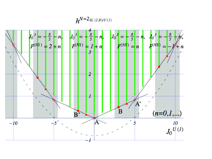
Figure 1: The unitary region of the $c_{KM}=8$ ($k_{\mbox{\scriptsize min}}=1$), $N=2$ superconformal algebra (NS sector). Green and red indicate, respectively, the continuous and discrete series representations contained in the spectrum.

We illustrate this in an example. FIG.1 shows the discrete-series representations of $N=2$ superconformal algebra associated with the noncompact coset for $k=\frac{6}{5}$ ($k_{\mbox{\scriptsize min}}=1$) in the NS-sector. The green lines are the continuous spectrum contained in the partition function, and the red points on the segments are the discrete states coming from the pole contributions. For the type II case, the points A and B only give massless states. They come from poles in the orbits $F_{0,0}$ and $F_{0,2}$ (after the isomorphisms), and with their superpartners they constitute a single vector- of a hyper-multiplet depending on the chirality. For the ($E_{8}\times E_{8}$) heterotic case, there are two additional points, A’ and B’, in the left mover which contribute to massless states. Various conformal weights of states which couple to these discrete states are shown in TABLE.I. It turns out that A (if paired with A in the right mover) gives $10\oplus 1$ and A’ does a singlet of $SO(10)$. With 16 states coming from the left Ramond sector, they constitute real scalars in the $27\oplus 1$ of $E_{6}$. B ,B’ and their corresponding left Ramond states yield another $27\oplus 1$. Ttaking into account their superpartners and the symmetry $\hat{F}_{l,2r}=\hat{F}_{k_{\rm min}-l,2r+k_{\rm min}+4}$, we find two ${\cal N}=1$ massless scalar multiplets in the $27\oplus 1$ of $E_{6}$ localized at the cigar tip.

No massless graviton is localized (nor massless gauge fields in the heterotic case), but if the noncompact Calabi-Yau is not the whole internal manifold itself but a part of some finite-size but large manifold compared to the scale of the collapsing cycles, which are isolated and distant from the rest, then there should be a massless graviton (and gauge fields for heterotic strings) associated with the constant mode, and they will interact with the localized fields. We hope that the singular CFT compactifications we presented here will lead to a new, interesting realization of local $E_{6}$ GUT with less moduli in this simple setting.

Table 1: Breakdowns of conformal weights constituting massless states for the $E_{8}\times E_{8}$ heterotic string ($k_{\mbox{\scriptsize min}}=1$, the left NS-sector).

Rep.	A	A’	B	B’
Lower bound	$0+\frac{5}{24}$	$\frac{5}{6}+\frac{5}{24}$	$\frac{3}{10}+\frac{5}{24}$	$\frac{2}{15}+\frac{5}{24}$
$N=2$ minimal	$0$	$\frac{1}{6}$	$0$	$\frac{1}{6}$
Imaginary momentum factor	$-\frac{5}{24}$	$-\frac{5}{24}$	$-\frac{1}{120}$	$-\frac{1}{120}$
$SO(10)$ fermions	$\frac{1}{2}$ or $0$	$0$	$\frac{1}{2}$ or $0$	$0$
Liouville fermions	$\frac{1}{2}$ or $0$	$0$	$0$ or $\frac{1}{2}$	$\frac{1}{2}$
$L_{0}^{SL(2,{\bf R})}$	$0$ or $1$	$0$	$0$	$0$
Total	$1$	$1$	$1$	$1$
$SO(10)$ representation	${\bf 10}\oplus{\bf 1}$	${\bf 1}$	${\bf 10}\oplus{\bf 1}$	${\bf 1}$

References

• (1) L. Susskind, “The anthropic landscape of string theory,” arXiv:hep-th/0302219. In “Carr, Bernard (ed.): Universe or multiverse?” 247-266.
• (2) G. W. Gibbons, “Aspects Of Supergravity Theories”. In Proceedings of the XVth GIFT International Seminar on Theoretical Physics, 123-146 (1984).
• (3) E. Witten, Phys. Rev. D44, 314-324 (1991).
• (4) R. Dijkgraaf, H. L. Verlinde and E. P. Verlinde, Nucl. Phys.  B 371, 269 (1992).
• (5) T. Eguchi and Y. Sugawara, JHEP 0501, 027 (2005).
• (6) I. R. Klebanov and M. J. Strassler, JHEP 08 (2000) 052; I. R. Klebanov and A. A. Tseytlin, Nucl. Phys. bf 578,123 (2000).
• (7) S. Mizoguchi, arXiv:0808.2857 [hep-th].
• (8) H. Ooguri and C. Vafa, Nucl. Phys.  B 463, 55 (1996) [arXiv:hep-th/9511164].
• (9) Y. Kazama and H. Suzuki, Nucl. Phys.  B 321, 232 (1989).
• (10) T. Eguchi and Y. Sugawara, JHEP 0405, 014 (2004) [arXiv:hep-th/0403193].
• (11) S. Mizoguchi, JHEP 0004, 014 (2000) [arXiv:hep-th/0003053]; arXiv:hep-th/0009240.
• (12) T. Eguchi and Y. Sugawara, Nucl. Phys.  B 577, 3 (2000). [arXiv:hep-th/0002100].
• (13) S. Murthy, JHEP 0610, 037 (2006). [arXiv:hep-th/0603121].
• (14) J. M. Maldacena, H. Ooguri and J. Son, J. Math. Phys.  42, 2961 (2001) [arXiv:hep-th/0005183].
• (15) D. Gepner, Phys. Lett.  B 199, 380 (1987). Nucl. Phys.  B 296, 757 (1988).
• (16) A. Hanany, N. Prezas and J. Troost, JHEP 0204, 014 (2002) [arXiv:hep-th/0202129].
• (17) W. Boucher, D. Friedan and A. Kent, Phys. Lett.  B 172, 316 (1986).
• (18) L. J. Dixon, M. E. Peskin and J. D. Lykken, Nucl. Phys.  B 325, 329 (1989).