Abstract

We compute the chains associated to the left-invariant CR structures on the three-sphere. These structures are characterized by a single real modulus $a$. For the standard structure $a=1$, the chains are well-known and are closed curves. We show that for almost all other values of the modulus $a$ either two or three types of chains are simultaneously present : (I) closed curves, (II) quasi-periodic curves dense on two-torii, or (III) chains homoclinic between closed curves. For $1<a<\sqrt{3}$ no curves of the last type occur. A bifurcation occurs at $a=\sqrt{3}$ and from that point on all three types of chains are guaranteed to exist, and exhaust all chains. The method of proof is to use the Fefferman metric characterization of chains, combined with tools from geometric mechanics. The key to the computation is a reduced Hamiltonian system, similar to Euler’s rigid body system, and depending on $a$, which is integrable.

1 Introduction and Results.

The left-invariant CR structures on the three-sphere $S^{3}=SU(2)$ form a family of CR structures containing the standard structure. After the standard structure, these form the most symmetric CR structures possible in dimension 3. See Cartan [5]. The purpose of this note is to compute the chains for these structures. (Computations of Cartan curvature type invariants for the left-invariant CR structures can be found in [4]. )

The chains on a strictly pseudoconvex CR manifold are a family of curves on the manifold invariantly associated to its CR structure. Chains were defined by Cartan [5]and further elucidated by Chern-Moser [6], and Fefferman [9]. Chains play a role in CR geometry somewhat similar to that of geodesics in Riemannian geometry. The left-invariant CR structures on $S^{3}$ are strictly pseudoconvex. Our computation of the chains for these structures appears here, apparently for the first time.

The space of left-invariant structures on $S^{3}=SU(2)$ modulo conjugation is a half-line parameterized by a single real variable $a$. Any left-invariant CR structure is conjugate to one of those presented in the normal form below (section 2, equations ( 2), (3) ). The standard structure corresponds to $a=1$. Its chains are obtained by intersecting $S^{3}\subset\mathbb{C}^{2}$ with complex affine lines in $\mathbb{C}^{2}$. (See [10] for especially good visual descriptions.) In particular all chains for the standard structure are closed curves. Here is our main result:

Theorem 1.1

Consider the left-invariant CR structures on the three-sphere. They form a one-parameter space, with parameter $a$ and $a=1$ corresponding to the standard structure, as given by the normal form of section 2, equations ( 2), (3). Then, for all but a discrete set of values of $a$ two types of chains are present: closed chains and quasi-periodic chains dense on two-torii. The curves of each type are dense in $S^{3}$. A bifurcation occurs at $a=\sqrt{3}$ so that for $a>\sqrt{3}$ a third type of chain occurs, corresponding to a homoclinic orbit and which accumulates onto a periodic chain ( a geometric circle). For all $a>\sqrt{3}$ all three types of chains: periodic, quasi-periodic, and homoclinic are present and every chain is one of these three types. For $a<\sqrt{3}$ only the closed chains and quasi-periodic chains are present.

Remark. We have left open the possibility that for a finite set of $a\in[1,\sqrt{3}]$ all chains are closed.

The computations leading to the theorem are based on a construction of Fefferman [9], refined and generalized by Lee [12] and Farris [8]. Starting with a strictly pseudoconvex CR manifold $M$ the Fefferman construction yields a circle bundle $S^{1}\to X\to M$ together with a conformal class of Lorentzian metrics on $X$. The chains are then the projections to $M$ of the light-like geodesics on $X$. It follows that we can look for chains by solving Hamiltonian differential equations.

Once we have the Hamiltonian system for Fefferman’s metric, a simple picture from geometric mechanics underlies this theorem. For our left-invariant structures this Hamiltonian system is very similar to that of a free rigid body, but with configuration space being $SU(2)=S^{3}$ instead of the rotation group $SO(3)$. Like the rigid body, this Hamiltonian system is integrable. Its solutions – the chains – lie on torii, the Arnol’d-Liouville torii. As in the case of the rigid body, the non-Abelian symmetry group forces resonances between the a priori three frequencies on the torii: so that the torii are in fact two-dimensional, not the expected three dimensions, of $3=dim(S^{3})$. When the frequencies are rationally related we get closed chains. Otherwise we get the quasi-periodic chains. The phase portrait (figure 2 below) changes with $a$ and the bifurcation at $a=\sqrt{3}$ corresponds to the origin turning from an elliptic to a hyperbolic fixed point in a bifurcation sometimes known as the Hamiltonian figure eight bifurcation.

1.1 Outline

There are five steps to the proof of the theorem. The paper is organized along these steps.
0. Find the normal form for the left-invariant structures on $SU(2)$.
1. Compute the Fefferman metric on $SU(2)\times S^{1}$ for the left-invariant CR structures.
2. Reduce the Hamiltonian system for the Fefferman geodesics by the symmetry group $SU(2)\times S^{1}$.
3. Integrate the reduced system.
4. Compute the geometric phases ( holonomies) relating the full motion to the reduced motion.

We briefly describe the methods and ideas involved in each one of the steps above, and in so doing link that step to the section in which it is completed.

Step 0. Finding a normal form. (Section 2 ) In section 2 we derive the normal form (2), (3) for the left-invariant CR structures with single real parameter $a$. This normal form is well-known and standard. Its derivation is routine. The normal form can be found for example in Hitchin [11] p. 34, and especially the first sentence of the proof of Theorem 10 on p. 99 there. Hitchin provided no derivation of the normal form. For completeness we present the derivation on the normal form in section 2.

Step 1. Finding the Fefferman metric. (Section 3)

In section 3 we compute the Fefferman metric associated to our normal forms. We follow primarily [12]. Inverting this metric yields the Hamiltonian $H=H_{a}$ whose solution curves correspond to chains.

Step 2. Constructing the reduced dynamics. (Sections 5 and 4)The chains for the left-invariant CR structures are the projections to $S^{3}$ of the light-like geodesics for the metrics computed in step 1. These geodesics are solutions to Hamiltonian systems on $T^{*}(S^{3}\times S^{1})$ whose Hamiltonians we write $H=H_{a}:T^{*}(S^{3}\times S^{1})\to\mathbb{R}$. As with all “kinetic energy” Hamiltonians, $H$ is a fiber-quadratic function on the cotangent bundle. To specify that the geodesics are light like, we only look at those solutions with $H=0$. The Fefferman metrics are always invariant under the circle action. In our case of left-invariant CR structures the metrics are also invariant under the left action of $S^{3}=SU(2)$ (extended in the standard way to the cotangent bundle). Consequently we can reduce the Fefferman dynamics by the groups $S^{1}$ and $SU(2)$. This reduction is performed in sections 4 and 5. Section 5 provides generalities concerning reducing left-invariant flows on Lie groups, and as such helps to orient the overall discussion. In section 4 we compute the reduced flow. In order to perform the reduction fix the standard basis $e_{1},e_{2},e_{3}$ for the $su(2)$. Write its dual basis, viewed as left-invariant one-forms, as $\omega^{1},\omega^{2},\omega^{3}$. Write $(g,\gamma)$ for a point of $S^{3}\times S^{1}$ and $d\gamma$ for the one-form associated to the angular coordinate $\gamma$. Any covector $\beta\in T^{*}_{g,\gamma}(S^{3}\times S^{1})$ can be expanded as $\beta=M_{1}\omega^{1}(g)+M_{2}\omega^{2}(g)+M_{3}\omega^{3}(g)+Pd\gamma$ so we can write have $H=H(g,\gamma;M_{1},M_{2},M_{3},P)$. Left-invariance implies that $H$ does not depend on $g$ or $\gamma$ so we can think of the Hamiltonian as a function $H=H(M_{1},M_{2},M_{3},P)$ on $\mathbb{R}^{3}\times\mathbb{R}$. The Euclidean space $\mathbb{R}^{3}\times\mathbb{R}$ represents $su(2)^{*}\times\mathbb{R}^{*}$, the dual of the Lie algebra of our Lie group, $SU(2)\times S^{1}$. Equivalently, $\mathbb{R}^{3}\times\mathbb{R}$ is the quotient space $T^{*}(S^{3}\times S^{1})/(S^{3}\times S^{1})$. The reduced dynamics is a flow on this space. The coordinate function $P$ is the momentum map for the action of the circle factor and as such is constant along solutions for the reduced dynamics. The function $H$ generates the reduced dynamics: $\dot{M}_{i}=\{M_{i},H\}$ and $\dot{P}=\{P,H\}(=0)$ where $\{\cdot,\cdot\}$ is the ‘Lie-Poisson bracket’. See section 5.

Step 3. Solving the reduced dynamics. (Section 6) The phase portrait found in figures 1, and 2 summarizes the reduced dynamics. . The computations proceed as follows. The functions $P$ and $K=M_{1}^{2}+M_{2}^{2}+M_{3}^{2}$ are Casimirs for the Lie-Poisson structure, meaning that $\{K,h\}=\{P,h\}=0$ for any Hamiltonian $h$ used to generate the reduced dynamics. The solutions to the reduced dynamical equations thus lie on the curves formed by the intersections of the three surfaces $P=const.$, $K=const.$ and $H=0$ in $\mathbb{R}^{4}=\mathbb{R}^{3}\times\mathbb{R}$. For typical values of these constants , these curves are closed curves. At special values the curves may be isolated points, or may be singular, like in the case of the homoclinic eight (figure 2).

When $P=0$ we can solve for the dynamics explicitly. The corresponding chains are the left translates of a particular one-parameter subgroup in $G=S^{3}$. The case $P\neq 0$ can be reduced to $P=1$ by the following scaling argument. We have $H(\lambda M_{1},\lambda M_{2},\lambda M_{3},\lambda P)=\lambda^{2}H(M_{1},M_{2},M_{3},P)$. Up on $S^{3}\times S^{1}$ this scaling represents leaving positions alone and scaling momenta, and hence velocities. Thus the reduced solution curves with initial conditions $(\lambda M_{1},\lambda M_{2},\lambda M_{3},\lambda P)$ and those with initial conditions $(M_{1},M_{2},M_{3},P)$ represent the same geodesics, and so the same chains, just parameterized differently. Choosing $\lambda=1/P$ we can always scale the case $P\neq 0$ to the case $P=1$. Now we have a single Hamiltonian $h=H(M_{1},M_{2},M_{3},1)$ on the standard rigid body phase space $\mathbb{R}^{3}$. We represent the surface $h=0$ as a graph $M_{3}=q(M_{1},M_{2};a)$ over the $M_{1}M_{2}$ plane, where $q$ is an even quartic function of $M_{1},M_{2}$. We form the solution curves by intersecting this graph with the level sets of $K$. To simplify the analysis we project the resulting curves onto the $M_{1}M_{2}$ plane. A critical point analysis of $K$ restricted to the graph locates the bifurcation value $a=\sqrt{3}$ for the reduced phase portrait as described in theorem 1.

Step 4. Geometric phases. (Section 7) We follow the idea presented in the paper [14] in order to reconstruct the chains in $S^{3}$ from the reduced solution curves. Some mild modifications are needed to that idea, since our initial group is $SU(2)\times S^{1}$ rather than the group $SO(3)$ of that paper. Fix $P=1$ and a value of $K$ so that the reduced curve $C$ of step 1 is closed. The left action of $SU(2)\times S^{1}$ on $T^{*}(S^{3}\times S^{1})$ has a momentum map with values in $su(2)^{*}\times\mathbb{R}^{*}$ and solutions (chains) must lie on constant level sets of this momentum map. One factor of this momentum map is $P$ from steps 2 and 3 which we have set to $1$. Upon projecting the level set onto $T^{*}S^{3}$ via the projection $T^{*}S^{3}\times T^{*}S^{1}\to T^{*}S^{3}$ we obtain an embedded $S^{3}\subset T^{*}S^{3}$ (the graph of a right-invariant one-form) together with a projection onto the reduced phase space $\mathbb{R}^{3}\times\{1\}$ of step 3. The inverse image of $C$ under this projection is a two-torus, and all the chains whose reduced dynamics is represented by $C$ and whose momentum map has the given fixed value lie on this two-torus. One angle of this torus represents the reduced curve. The relevant question is: as we go once around the reduced curve, how much does the other angle change? Call this amount $\Delta\theta$. If the value of $\Delta\theta$ is an irrational multiple of $2\pi$ then the chain is not closed and forms one of the quasi-periodic chains of theorem 1, dense on its two-torus. If its value of $\Delta\theta$ is a rational multiple $p/q2\pi$ of $2\pi$ then the chain is closed, corresponding to some $p,q$ winding on its torus. With certain modifications, the basic integral formula for $\Delta\theta$ from [14] is valid. One term in this formula corresponds to a holonomy of a connection, and is termed the “geometric phase”, explaining the subtitle we have given to this step 4. The values of $\Delta\theta$ depends only on the values of $a$ and $K$ and its dependence is analytic in these variables. Thus the proof of the theorem will be complete once we have shown there is a value of $a$ for which $K\mapsto\Delta\theta(K,a)$ is not constant.

In order to prove non-constancy of $\Delta\theta(K,a)$ , take $a>\sqrt{3}$ so that the reduced dynamics has a homoclinic eight. Denote the value of $K$ on the eight by $k(a)$. We show that as $K\to k(a)$ we have that $\Delta\theta(a,K)\to\infty$.

Steps 0–4 now completed, theorem 1 is proved.

Appendices. We finish the paper with two appendices. In appendix A we verify that when $a=1$ the Fefferman geodesics for the Hamiltonian computed here (eq. 26) correspond to the well-known chains for the standard three-sphere. In appendix 2 we show that the left-invariant CR structures for $a\neq 1$ correspond to the family of non-embeddable CR structures on $S^{3}$ discovered by Rossi, and frequently found in the CR literature.

An Open problem. We end appendix B with an open problem inspired by the Rossi embedding of $S^{3}/(\hbox{antipodal map})$ and a conversation with Dan Burns.

2 A normal form for the left-invariant CR structures (step 0).

2.1 Preliminaries. Basic Definitions.

A contact structure in dimension 3 is defined by the vanishing of a one-form $\theta$ having the property that $\theta\wedge d\theta\neq 0$. Let $M$ be the underlying 3-manifold and $TM$ its tangent bundle. The contact structure is the field of 2-planes $\xi=\{(m,v)\in TM:\theta(m)(v)=0\}\subset TM$. It is a rank 2 sub-bundle of the tangent bundle. The one-form $\theta$ and $f\theta$, for $f\neq 0$ a function, define the same contact structure.

Definition 2.1

A strictly pseudoconvex CR structure on a 3-manifold $M$ consists of contact structure $\xi$ on $M$ together with an almost complex structure $J$ defined on the contact planes $\xi$.

We will primarily be using the following alternative, equivalent definition

Definition 2.2

A strictly pseudoconvex CR structure on a 3-manifold $M$ consists of an oriented contact structure $\xi$ on $M$ together with a conformal equivalence class of metrics defined on contact planes $\xi$.

To pass from the first definition to the second, we construct the conformal structure from the almost complex structure $J$ in the standard way. Namely, the conformal structure is determined by knowing what an orthogonal frame is, and we declare $e,J(e)$ to be such a frame, for any nonzero vector $e\in\xi$. An alternative to this construction is to choose a contact form $\theta$ for the contact structure and then construct its associated Levi form

$$L_{\theta}(v,w)=d\theta(v,Jw)$$ (1)

which is a quadratic symmetric form on the contact planes. The contact condition implies that the Levi form is either negative definite or positive definite. If it is negative definite, replace $\theta$ with $-\theta$ to make it positive definite. We henceforth insist that $\theta,J$ are taken so the Levi form is positive definite. This assumption on $(\theta,J)$ is equivalent to assuming that the orientation on the contact planes induced by $\theta$ and $J$ agree. (Note that a choice of contact one-form orients the contact planes. ) The conformal structure associated to $(\theta,J)$ from definition 2.1 is generated by the Levi form. If we change $\theta\to f\theta$ with $f>0$ then the Levi form changes by $L_{\theta}\to fL_{\theta}$, showing that this definition of conformal structure is independent of (oriented) contact form $\theta$.

To go from definition 2.2 to definition 2.1, take any oriented orthogonal basis vectors $E_{1},E_{2}$ having the same length relative to some metric in the conformal class. Define $J$ by $J(E_{1})=E_{2},J(E_{2})=-E_{1}$. Thus in dimension 3 we can define a CR structure by a contact form $\theta$, defined up to positive scale factor, together with an inner product on the contact planes $\omega=0$ to represent the conformal structure, also only defined up to a positive scaling. Choosing the scale factor of either the contact form or the quadratic form fixes the scalar factor of the other one through the Levi-form relation, eq. (1).

2.2 The left-invariant case.

We take $M=S^{3}$ which we identify with the Lie group $SU(2)$ in the standard way, via the action of $SU(2)$ on $S^{3}\subset\mathbb{C}^{2}$. A left-invariant CR structure on $S^{3}$ is then given by Lie algebraic data on $su(2)$. This data consists of a ray in $su(2)^{*}$ representing the left-invariant contact form $\theta$ up to positive scale and a quadratic form on $su(2)$ defined modulo $\theta$, and positive definite when restricted to $ker(\theta)$. Conjugation on $SU(2)$ maps left invariant CR structures to left-invariant CR structures, and induces the co-adjoint action on $su(2)^{*}$. This action is equivalent, as a representation, to the standard action of the rotation group $SO(3)$ on $\mathbb{R}^{3}$ via the 2:1 homomorphism $SU(2)\to SO(3)$. Consequently, we can rotate the contact form $\theta$ to anti-align with the basis element $\omega_{3}$. Thus we take $\theta=-\omega^{3}$. The contact planes are then framed by the left-invariant vector fields $e_{1},e_{2}\in su(2)$. The choice of $-\omega^{3}$ is made so that $e_{1},e_{2}$ is the correct orientation of the plane, as follows from the structure equation

$$d\omega^{3}=-\omega^{1}\wedge\omega^{2}.$$

This structure equation also proves that the plane field $-\omega^{3}=0$ is indeed contact, so that the corresponding CR structure (no matter the choice of $J$) will be strictly pseudoconvex. A quadratic form on the contact plane is given by a positive definite quadratic expression in $\omega^{1},\omega^{2}$ , that is: $A(\omega^{1})^{2}+2B\omega^{1}\omega^{2}+C(\omega^{2})^{2}$, viewed mod $\omega^{3}$. The isotropy group of $\omega^{3}$ acts by rotations of the contact plane (the $e_{1},e_{2}$ plane). A quadratic form can be diagonalized by rotations, so upon conjugation by some element of the isotropy subgroup of $\omega^{3}$ we can put the quadratic form in the diagonal form $A(\omega^{1})^{2}+B(\omega^{2})^{2}$ with $A,B>0$. The form is only well-defined up to scale, and we can scale it so that $A=1/B$, i.e the conformal structure is that of $(1/a)(\omega^{1})^{2}+a(\omega^{2})^{2}$, $a>0$. We have proved the bulk of :

Proposition 2.1 (Normal form)

Every left-invariant CR structure on $S^{3}$ is conjugate to one whose contact form is given by

$$\theta=-\omega^{3}$$ (2)

and whose associated conformal structure is

$$L_{\theta}=\frac{1}{a}(\omega^{1})^{2}+a(\omega^{2})^{2}$$ (3)

The associated almost complex structure $J=J_{a}$ is defined by $J(e_{1})={1\over a}e_{2}$, $J(e_{2})=-ae_{2}$. The structure defined by $a$ is isomorphic to the structure defined by $1/a$. As the notation indicates, the quadratic form $L_{\theta}$ is indeed the Levi-form associated to $\theta,J$ as per eq. (1).

To see that $J$ in the proposition is correct, note that the choice $\theta=-\omega^{3}$ as contact form induces the orientation $\{e_{1},e_{2}\}$ to the contact planes, and that $\left\{e_{1},{1\over a}e_{2}\right\}$ are orthogonal vectors having the same squared length ($1/a$)relative to the given metric $L_{\theta}$. To see that the structure defined by $a$ is isomorphic to the structure defined by ${1\over a}$ observe that rotation by 90 degrees converts $(1/a)(\omega^{1})^{2}+a(\omega^{2})^{2}$ to $a(\omega^{1})^{2}+(1/a)(\omega^{2})^{2}$. Finally, compute from $d\theta=\omega^{1}\wedge\omega^{2}$ and the form of $J$ that indeed, the Levi form is the given quadratic form $L_{\theta}$.

3 Fefferman’s metric (step 1).

When the strictly convex CR structure on $M$ is induced by an embedding $M\subset\mathbb{C}^{2}$, Fefferman [9] constructed a circle bundle $Z\to M$ together with a conformal Lorentzian metric on $Z$ invariantly associated to the CR structure. Farris [8] and then Lee [12] generalized Fefferman’s construction to the case of an abstract strictly pseudoconvex CR structure, i.e. one not necessarily induced by an embedding into $\mathbb{C}^{2}$. In this section we construct the Fefferman metric for the family of left-invariant CR structures from step 1 (proposition 2.1 there). We most closely follow Lee’s presentation.

We begin with a general construction. Let $\pi:Z\to M$ be any circle bundle over $M$. Fix a contact form $\theta$. Recall that the Reeb vector field associated to $\theta$ is the vector field on $M$ uniquely defined by the two conditions

$$\theta(R)=1$$

$$i_{R}d\theta=0.$$

Changing $\theta$ to $g\theta$, $g$ a function, changes $R$ to ${1\over g}R+X_{g}$ where $X_{g}$ lies in the contact plane field and is determined pointwise by a linear equation involving $dg$ and $d\theta$ which is reminiscent of the equation relating a Hamiltonian to its Hamiltonian vector field. We extend the Levi form (1) to all of $TM$ by insisting that $L_{\theta}(R,v)=0$ for all $v\in TM$ and continue to write $L_{\theta}$ for this extended form. Let $\sigma$ be any one-form on $Z$ with the property that $\sigma$ is nonzero on the vertical vectors (the kernel of $d\pi$). Then

$$g_{\theta}=\pi^{*}L_{\theta}+4(\pi^{*}\theta)\odot\sigma$$ (4)

is a Lorentzian metric on $Z$. Here $\odot$ denotes the symmetric product of one-forms: $\theta\odot\sigma=\frac{1}{2}(\theta\otimes\sigma+\sigma\otimes\theta)$.

The trick needed is a way of defining $\sigma$ in terms of the contact form, and $J$, in such a way that a “conformal change” $\theta\mapsto g\theta$ of the contact structure induces a conformal change of the metric $g_{\theta}$.

Warning. Farris and Lee, use a different definition of the symmetric product $\odot$: their $\theta\odot\sigma$ is twice ours, so that in their formula for the metric our $4$ is replaced by a $2$. We have chosen our definition so that, using it, $(dx+dy)^{2}=dx^{2}+2(dx\odot dy)+dy^{2}$, where $\theta^{2}=\theta\otimes\theta$.

3.1 Forming the circle bundle from the canonical bundle. (2,0) forms.

The circle bundle $Z\to M$ will be a bundle of complex-valued 2-forms, defined up to real scale factor. A choice of contact form $\theta$ on $M$ induces various one-forms on $Z$ in a canonical way. One of these one-forms will be the form $\sigma$ needed for the Fefferman metric, eq. (4). Here are the main steps leading to the construction of $Z$ and its one-form $\sigma$.

The complexified contact plane $\xi_{\mathbb{C}}=\xi\otimes\mathbb{C}$ splits under $J$ into the holomorphic and anti-holomorphic directions, these being the $+i$ and $-i$ eigenspaces of $J$, where $J$ is extended from $\xi$ to $\xi_{\mathbb{C}}$ by complex linearity. In the case of 3-dimensional CR manifold, if we start with any non-zero vector field $E$ tangent to $\xi$, then $Z=E-iJE$ spans the holomorphic direction, while $\bar{Z}=E+iJE$ spans the anti-holomorphic direction. In our case

$$Z_{a}=e_{1}-{i\over a}e_{2}$$ (5)

is holomorphic, while

$$\bar{Z}_{a}=e_{1}+{i\over a}e_{2}$$ (6)

is the anti-holomorphic vector field.

Remark. Third definition of a 3-dimensional CR manifold. Eq. (5) corresponds to yet a third definition of a CR manifold.

Definition 3.1

(CR structure, 3rd time ’round). A CR structure on $M^{3}$ is a complex line field, i.e. a rank 1 subbundle of the complexified tangent bundle $TM\otimes{\mathbb{C}}$ which is nowhere real.

Such a complex line field is locally spanned by a “holomorphic” vector field $Z$ as in eq. (5). Writing $Z=E_{1}-iE_{2}$ with $E_{1},E_{2}$ real vector fields, we define the 2-plane field $\xi$ to be the real span of $E_{1},E_{2}$, and we set $J(E_{1})=E_{2}$, $J(E_{2})=-E_{1}$. The “strictly pseudoconvex” condition, which is the condition that $\xi$ be contact, is that $E_{1},E_{2}$ together with the Lie bracket $[E_{1},E_{2}]$ span the real tangent bundle $TM$.

The almost complex structure $J$ on the contact planes of a CR manifold induces a splitting of the space of complex-valued differential forms into types $\Omega^{p,q}$ similar to the splitting of forms on a complex manifolds. We declare that a complex valued k-form $\beta$ is of type $(k,0)$ (that is to say “holomorphic”) if $i_{\bar{Z}}\beta=0$ for all anti-holomorphic vector fields $\bar{Z}$. In dimension $3$, one only needs to check this equality for a single nonzero such vector field, such as $\bar{Z}$ of eq. ( 6).

Our case. The space of (1,0) forms for the left-invariant structure for the parameter value $a$ is spanned by,

$$\theta=-\omega^{3}\;;\omega_{a}=\omega^{1}+ia\omega^{2}\,\,\hskip 42.67912pt:(1,0)\hbox{ forms }.$$ (7)

The (2,0) forms are spanned (over $\mathbb{C}$) by

$$\theta\wedge\omega_{a}\,\,\,\hskip 42.67912pt:(2,0)\hbox{ forms }.$$ (8)

In dimension 3 the space of all $(2,0)$ forms, considered pointwise, forms a complex line bundle, denoted by $K$ and called the canonical bundle as in complex differential geometry. $Z$ is defined to be the “ray projectivization” of $K$:

$$Z=K\setminus\{\hbox{ zero section }\}/\mathbb{R}^{+}.$$

We next recall from Lee [12] how a choice of contact form $\theta$ determines the one-form $\sigma$ on $Z$.

1. Volume normalization equation. Fix the contact form $\theta$ on $M$. The volume normalization equation is

$$\sqrt{-1}\textrm{ }\theta\wedge i_{R}\zeta\wedge i_{R}\bar{\zeta}=\theta\wedge d\theta.$$ (9)

The right hand side is the standard volume form defined by a choice of contact structure. On the left-hand side, $R=R_{\theta}$ is the Reeb vector field for $\theta$. The 2-form $\zeta\in\Gamma(K)$, a section of the canonical bundle is to viewed as the unknown. The equation is quadratic in the unknown since multiplying $\zeta$ by the complex function $f$ multiplies the left hand side of the volume normalization equation by $|f|^{2}$. It follows by this scaling that there is a solution, $\zeta_{0}$ to the volume normalization which is unique up to unit complex multiple $\zeta\mapsto e^{i\gamma}\zeta$.

Said slightly differently, eq. (9) defines a section

$$s=s_{\theta}:Z\to K$$

of the ray bundle $K\to Z$, since once we fix the complex phase of $\zeta$, the equation uniquely determines the real scaling factor. Fix a solution, which is to say, a smoothly varying pointwise choice of solutions

$$\zeta_{0}:M\to K$$

to eq. (9). Such a solution choice defines a global trivialization of $Z$, since we can express any point $z$ of $Z$ (uniquely) as

$$s_{\theta}(z)=e^{i\gamma}\zeta_{0}(\pi(z))$$

where $m=\pi(z)\in M$. Thus the choice $\zeta_{0}$ induces a global trivialization:

$$Z\cong M\times S^{1}.$$

(A more pictorial, equivalent description of this trivialization of $Z$ is as follows. Form the ray generated by $\zeta_{0}(m)$, which is a point in the circle fiber $Z_{m}$, over $m$. Rotate this ray by the angle $\gamma$ until you hit the ray $z\in Z_{m}$, thus associating to $z$ a point $(m,\gamma)\in M\times S^{1}$).
We henceforth use this identification $Z=M\times S^{1}$ and define a global one-form on $Z$ by

$$\zeta(m,\gamma)=e^{i\gamma}\zeta_{0}(m).$$ (10)

We check now that the two-form $\zeta$ depends only on the choice of contact form $\theta$, and so, up to this choice, is intrinsic to $Z$. The total space $K$ of the canonical bundle , like any total space constructed as a bundles of $k$-forms, has on it a canonical $k$-form $\Xi$. To describe $\Xi$ write a typical point of $K$ as $(m,\beta)\in K$, $m\in M$, $\beta\in\Lambda^{(2,0)}T_{x}M$. Then we can set $\Xi(x,\beta)=\pi_{x}^{*}\beta$ where $\pi:K\to M$ denotes the projection. This canonical form, like all such canonical forms, enjoys the reproducing property that if $\beta:M\to K$ is any section, then $\beta^{*}\Xi=\beta$. Let $s=s_{\theta}:Z\to K$ to pull back $\Xi$:

$$\zeta:=s_{\theta}^{*}\Xi,\textrm{ a (2,0)-form on $Z$}.$$

The reproducing property shows that, under the global trivialization of $Z$ induced by $\zeta_{0}$, we have that $\zeta$ is given by formula (13) below.

Our case. Return to the left-invariant situation: Choosing $\theta=-\omega^{3}$ we get $\theta\wedge d\theta=-\omega^{1}\omega^{2}\omega^{3}$. The associated Reeb field is

$$R=-e_{3}.$$ (11)

Writing $\zeta_{0}=g\theta\wedge\omega_{a}$ we compute that $i_{R}\zeta_{0}=g\omega_{a}$. Using $\omega_{a}\wedge\bar{\omega}_{a}=-2ia\omega^{1}\wedge\omega^{2}$ we compute that the left-hand side of the volume normalization equation (9) expands out to $-2a|g|^{2}\omega^{1}\omega^{2}\omega^{3}$. The volume normalization equation (9) then implies that $|g|^{2}=1/2a$. Thus

$$\zeta_{a}=\frac{1}{\sqrt{2a}}\theta\wedge\omega_{a}$$ (12)

is a global normalized section of $K$. It induces a global trivialization of $Z$, as just described, so that we can think of $Z$ as $S^{3}\times S^{1}$. With $(m,e^{i\gamma})$ being the ray through the (2,0) form $e^{i\gamma}\zeta_{a}(m)$. The two-form $\zeta$ on $Z$ is given, under this identification, by this same algebraic relation:

$$\zeta=e^{i\gamma}\frac{1}{\sqrt{2a}}\theta\wedge\omega_{a}$$ (13)

where we are not using different symbols to differentiate between a form $\beta$ on $M$ and its pull-backs $\pi^{*}\beta$ to $Z$.

Proposition 3.1 (Lee: [12], p. 417)

Fix the contact form $\theta$ for the CR manifold $M$. Let $\zeta$ be the induced one-forms on $Z$ as just described. Let $R$ be the Reeb vector field for $\theta$.

A. There is a complex valued one-form $\eta$ on $Z$, uniquely determined by the conditions: .

$$\zeta=\theta\wedge\eta$$ (14)

$$i_{v}\eta=0\hbox{ whenever }\pi_{*}v=R$$ (15)

B. With $\eta$ as in A, there is a unique real-valued one form $\sigma$ on $Z$ determined by the equations

$$d\zeta=3i\sigma\wedge\zeta$$ (16)

$$\sigma\wedge d\eta\wedge\bar{\eta}=Tr(d\sigma)i\sigma\wedge\theta\wedge\eta\wedge\bar{\eta}.$$ (17)

The meaning of $`Tr^{\prime}=$Trace in this last equation is as follows. Any solution $\sigma$ to (16) has the property that $d\sigma$ is basic, i.e. is the pull-back of a two-form on $M$, which by abuse of notation we also denote by $d\sigma$. Any two-form on $M$ can be expressed as $fd\theta+\theta\wedge\beta$. Set $Tr(fd\theta+\theta\wedge\beta)=f$.

C. The form $\sigma=\sigma(\theta)$ determined by the equations (14, 15, 16, 17) is the form $\sigma$ appearing in the Fefferman metric $g_{\theta}$ of eq. (4). If $\theta\mapsto f\theta$, $f>0$ then the Reeb extended Levi form $L_{\theta}$ and $\sigma$ transform in such a way that $g_{f\theta}=fg_{\theta}$, i.e. the conformal class of the Fefferman metric is indeed invariantly attached to the CR structure.

Remark. An equivalent definition of the trace used in eq (17) is as follows. Take a two-form such as $d\sigma$ on $M$, restrict it to the contact plane and then use the Levi form $L_{\theta}$ to raise its indices and thus define its trace, $Tr(d\sigma)$.

The forms on $Z$ in the left-invariant case. In our left-invariant situation the forms $\theta,\zeta$ of the theorem have been described above in equations (2), (13). They are $\theta=-\omega^{3}$, $\zeta=\theta\wedge\eta$ with

$$\eta=\frac{1}{\sqrt{2a}}(e^{i\gamma}\omega_{a})$$ (18)

and

$$\omega_{a}=(\omega^{1}+ia\omega^{2})$$

This $\eta$ is indeed the $\eta$ of part A of the theorem, since if $V$ is any vector field on $Z$ satisfying $\pi_{*}V=R$ then $i_{V}\pi^{*}\eta=i_{R}\eta=0$. (Recall we use $\eta$ for $\pi^{*}\eta$ as forms on $Z$.)

Now we move to the computations of part B of the Proposition for the one-form $\sigma$. We compute:

$$\sigma={{d\gamma}\over{3}}+f\theta\hskip 14.22636pt,\hskip 14.22636ptf=\frac{1}{8}(a+1/a).$$ (19)

Here are key steps along the way of the computation:

$$d\eta=id\gamma\wedge\eta+\frac{1}{\sqrt{2a}}e^{i\gamma}d\omega_{a}$$ (20)

$$=id\gamma\wedge\eta+\frac{1}{\sqrt{2a}}e^{i\gamma}\theta\wedge(-\omega^{2}+ia\omega^{1}).$$ (21)

Then

$$d\zeta=id\gamma\wedge\zeta$$

It then follows from the first equation in part B of the theorem, and the reality of $\sigma$ that

$$\sigma=\frac{d\gamma}{3}+f\theta$$

for some real function $f$. We have $Tr(d\sigma)=f$. Setting $dvol=d\gamma\wedge\theta\wedge\omega^{1}\wedge\omega^{2}$ we compute the right hand side of eq. (17) to be $(f/3)dvol$, while its left hand side is equal to $[(1/3)(1+a^{2})/2a-f]dvol$. Setting the two 4-forms equal and solving for $f$ yields $f=(1+a^{2})/8a$ as claimed.

Returning now to the form of the Fefferman metric, eq. (4), and using $\theta=-\omega^{3}$ we see that the metric is given (up to conformality) by

$$ds^{2}=\{{1\over a}(\omega^{1})^{2}+a(\omega^{2})^{2}\}+4\omega^{3}\odot(\frac{1}{8}(a+\frac{1}{a})\omega^{3}-{{d\gamma}\over{3}}).$$ (22)

Written in terms of the basis $\{e_{1},e_{2},e_{3},{\partial\over{\partial\gamma}}\}$ this metric is

$$g(a)=\left(\begin{array}[]{cccc}\frac{1}{a}&0&0&0\\ 0&a&0&0\\ 0&0&\frac{1}{2}(a+\frac{1}{a})&-\frac{2}{3}\\ 0&0&-\frac{2}{3}&0\end{array}\right).$$ (23)

4 Reduced light ray equations (step 2.)

The geodesics for any metric $ds^{2}=\Sigma g_{ij}dx^{i}dx^{j}$, Riemannian or Lorentzian, can be characterized as the solutions to Hamilton’s equations for the Hamiltonian defined by inverting the metric, and viewing the result as a fiber quadratic function on the cotangent bundle:

$$H(x,p)={1\over 2}\Sigma g^{ij}(x)p_{i}p_{j}.$$ (24)

(See for example, [1], [2], or [13].) Here $g^{ij}(x)$ is the matrix pointwise inverse to the matrix with entries $g_{ij}(x)$.

If we are only interested in light-like geodesics, then we restrict to solutions for which $H=0$. It is important that these geodesics are conformally invariant. If $\tilde{d}s^{2}=fds^{2}$ is a metric conformal to the original, then the corresponding Hamiltonians are related by $\tilde{H}=H/f$ and the two Hamiltionian vector fields, are related on their common zero level set $\{H=0\}$ by $X_{\tilde{H}}=(1/f)X_{H}$. This proportionality of vector fields says that the set of light rays for any two conformally related metrics $ds^{2},\tilde{d}s^{2}$ are the same as sets of unparameterized curves.

The Hamiltonian for the Fefferman metric lives on $T^{*}Z$. Any covector $p\in T^{*}_{z}Z$ can be expanded in the basis $\omega_{1},\omega_{2},\omega_{3},d\gamma$ dual to the basis in which the matrix (23) was computed:

$$p=M_{1}\omega_{1}+M_{2}\omega_{2}+M_{3}\omega_{3}+Pd\gamma$$

The inverse matrix to (23) is

$$g^{-1}(a)=\left(\begin{array}[]{cccc}a&0&0&0\\ 0&{1\over a}&0&0\\ 0&0&0&-3/2\\ 0&0&-3/2&-\frac{9}{8}(a+\frac{1}{a})\end{array}\right).$$ (25)

It follows that the Fefferman Hamiltonian for our left-invariant CR structure with parameter $a$ is given by

$$H_{a}(g,\gamma;M_{1},M_{2},M_{3},P)=\frac{1}{2}\{aM_{1}^{2}+{1\over a}M_{2}^{2}-3M_{3}P-\frac{9}{8}(a+\frac{1}{a})P^{2}\}.$$ (26)

5 Left-invariant geodesic flows.

Our Hamiltonian (26, 23) generates the geodesic flow for a left-invariant (Lorentzian) metric on the Lie group $G=SU(2)\times S^{1}$. In this section we review some general facts regarding left-invariant geodesic flows, and specify to our situation. We refer the reader to [1], especially chapter 4, or [2], especially Appendix 2, for background and more details regarding the material of this section and the next.

5.1 Generalities

Let $Q$ be a manifold. Let $ds^{2}$ be a metric on $Q$ as above. The geodesic flow for $ds^{2}$ is encoded by a Hamiltonian vector field $X$ on $T^{*}Q$ which is defined in terms of the Hamiltonian above in eq. (24). The vector field $X$ can be defined by the canonical Poisson brackets $\{,\}$ on $T^{*}Q$ according to $X[f]=\{f,H\}$, for $f$ any smooth function on $T^{*}Q$. It is worth noting that the momentum scaling property $H(q,\lambda p)=\lambda^{2}H(q,p)$, for $p\in T^{*}_{q}Q$ corresponds to the fact that the geodesic $\tilde{\gamma}(t)$ with initial conditions $(q,\lambda p)$ is simply the same geodesic $\gamma(t)$ as represented by the initial conditions $(q,p)$ but just parameterized at a different speed: $\tilde{\gamma}(t)=\gamma(\lambda t)$

Now suppose that $Q=G$ is a finite dimensional Lie group and the metric is left-invariant, i.e. left translation by any element of $G$ acts by isometries relative $ds^{2}$. The left action of $G$ on itself canonically lifts to $T^{*}G$, and left-invariance of the metric implies that the Hamiltonian $H$ is left-invariant under this lifted action. Write $\mathfrak{g}$ for the Lie algebra of $G$, and $\mathfrak{g}^{*}$ for the dual vector space to $\mathfrak{g}$, which we identify with $T^{*}_{e}G$, where $e\in G$ is the identity. Using the codifferential of left-translation, we left-trivialize $T^{*}G=G\times\mathfrak{g}^{*}$, and use corresponding notation $(g,M)\in G\times\mathfrak{g}^{*}$ for points in the trivialized cotangent bundle. Then the left-invariance of $H$ means that, relative to this trivialization we have

$$H(g,M)=H(M)$$

depending on $M$ alone.

Let $e_{a}$ be a basis for $\mathfrak{g}$, the Lie algebra of $G$, and $\omega^{a}$ the corresponding dual basis for $\mathfrak{g}^{*}$. Then we can expand

$$M=\Sigma M_{a}\omega^{a}$$

and

$$H={1\over 2}\Sigma g^{ab}M_{a}M_{b}$$

where $g^{ab}$ is the matrix inverse to the inner product matrix $g_{ab}=ds^{2}(e_{a},e_{b})$. We find that

$$\{M_{a},M_{b}\}=-\Sigma c^{d}_{ab}M_{d}$$

where $c^{d}_{ab}$ are the structure constants of $\mathfrak{g}$ relative to the basis $e_{a}$.

It follows that the geodesic flow can be pushed down to the quotient space $(T^{*}G)/G=\mathfrak{g}^{*}$, and as such it is represented in coordinates by

$$\dot{M}_{a}=-\Sigma_{k,b,r}g^{rb}c^{k}_{ab}M_{r}M_{k}$$

We will call these the “reduced equations”, or “Lie-Poisson equations”. They are a system of ODE’s on $\mathfrak{g}^{*}$. We will call the quotient map $T^{*}G\to(T^{*}G)/G=\mathfrak{g}^{*}$ the reduction map. (Warning: This map is not the reduction map of symplectic reduction.)

5.1.1 Momentum Map

The left-action of $G$ on itself, lifted to $T^{*}G$ has for its momentum map the map $J:T^{*}G\to\mathfrak{g}^{*}$ of right trivialization. In terms of our left-trivialized identification $J(g,M)=Ad_{g^{-1}}^{*}M$ where $Ad_{g}^{*}:\mathfrak{g}^{*}\to\mathfrak{g}^{*}$ denotes the dual of the adjoint representation $Ad_{g}$ of $G$ on $\mathfrak{g}$. The left-invariance of $H$ implies that each integral curve for the Hamiltonian vector field $X$, i.e. the geodesics, when viewed as curves in the cotangent bundle, lies within a constant level set of $J$.

Each individual constant level-set $J^{-1}(\mu)$ is the image of a right-invariant one-form $G\to T^{*}G$, and as such is a copy of $G$ in $T^{*}G$. The projection of such a level set onto $\mathfrak{g}^{*}$ by the reduction map yields as image the co-adjoint orbit through $\mu$ , thus: $\pi(J^{-1}(\mu))=G\cdot\mu$ where $G\cdot\mu=\{M:M=Ad_{g}^{*}\mu,g\in G\}\subset\mathfrak{g}^{*}$. Since the integral curves in $T^{*}G$ lie on level sets of $J$, the integral curves of the reduced dynamics lie on such co-adjoint orbits.

5.1.2 Unreducing

Let $G_{\mu}$ denote the isotropy group of $\mu\in\mathfrak{g}^{*}$ under the co-adjoint action. As smooth $G$-spaces we have $\pi(J^{-1}(\mu))=G\cdot\mu=G/G_{\mu}$ , and the projection of $J^{-1}(\mu)\to\pi(J^{-1}(\mu))$ is isomorphic to the canonical bundle projection $G\to G/G_{\mu}$ with fiber $G_{\mu}$. When $G$ is compact then for generic $\mu$ we have that $G_{\mu}\cong T$, where $T$ is the maximal torus $T$ of $G$ and the rank $r$ of $G$ is the dimension of $T$. If the typical integral curves $C$ for the reduced dynamics are closed curves $C\subset G\cdot\mu\subset\mathfrak{g}^{*}$, then the integral curves for the original dynamics sit on manifolds $\pi^{-1}(C)\cap J^{-1}(\mu)$ which is a $T$-bundle over the circle $C$. In our particular situation this bundle will be trivial, so that $\pi^{-1}(C)\cap J^{-1-}(\mu)$ is itself a torus of one more dimension than $T$.

5.1.3 Casimirs

A Casimir on $\mathfrak{g}^{*}$ is a smooth function such that for all smooth functions $h$ on $\mathfrak{g}^{*}$ we have that $\{C,h\}=0$. The values of a Casimir stay constant on the solutions to the reduced equation. For $G$ compact with maximal torus $T$ the algebra of Casimirs is functionally generated by $r$ polynomial generators, these generators being polynomials invariant under the co-adjoint action. The common level set $C_{1}=c_{1},\ldots,C_{r}=c_{r}$ of these $r$ Casimirs is, for generic values of the constants $c_{i}$, a co-adjoint orbit $G\cdot\mu$ for which $G_{\mu}=T$.

5.2 The case of Lorentzian metrics on $SU(2)\times S^{1}$

The Hamiltonian for the Fefferman metric (eq. 26) computed from step 1 is that of a left-invariant Lorentzian metric on $G=SU(2)\times S^{1}$. We specialize the discussion of the last few paragraphs to this situation. Then the dual of the Lie algebra of $G$ splits as $\mathfrak{g}^{*}=\mathbb{R}^{3}\times\mathbb{R}$. The $\mathbb{R}^{3}$ factor acts like the well-known angular momentum from physics. The coordinates $M_{1},M_{2},M_{3},P$ appearing in eq. (26) are linear coordinates on $\mathfrak{g}^{*}=\mathbb{R}^{3}\times\mathbb{R}$. . Their Lie-Poisson brackets are

$$\{M_{1},M_{2}\}=-M_{3},\hskip 5.69046pt\{M_{3},M_{1}\}=-M_{2},\hskip 5.69046pt\{M_{2},M_{3}\}=-M_{1}$$

together with

$$\{M_{i},P\}=0.$$

The rank $r$ of $G$ is $2$. The algebra of Casimirs is generated by

$$P\hbox{ and }K=M_{1}^{2}+M_{2}^{2}+M_{3}^{2}\hskip 8.5359pt\hbox{ (Casimirs) }$$

Using momentum scaling, we can split the analysis of the reduced geodesic flow into two cases, $P=0$, and $P=1$.

5.2.1 Case 1: $P=0$

We will see that our Hamiltonian equations for this first case are easily solved. The reduced dynamics will be trivial: $M_{1}=M_{2}=0$, $M_{3}=const$. Up on $G$, the corresponding geodesics are left translates of the one-parameter subgroup corresponding to the third direction.

5.2.2 Case 2: $P=1$

When $P=1$ we have for our Hamiltonian the function $H(M,1)$ on $\mathbb{R}^{3}=\mathbb{R}^{3}\times\{1\}\subset\mathfrak{g}^{*}$. We are only interested in the light-like geodesics, which means we will set $H(M,1)=0$. This defines a paraboloid in $\mathbb{R}^{3}$. The integral curves for the reduced dynamics lie on the intersections of this paraboloid with the spheres $K=r_{0}^{2}$. These intersections typically consist of one or two closed curves, which are the closed integral curves of the reduced dynamics.

5.2.3 Co-adjoint action and identifications

The co-adjoint action of $G$ on $\mathfrak{g}^{*}=\mathbb{R}^{3}\times\mathbb{R}$ acts trivially on the $\mathbb{R}$ factor, since that corresponds to the Abelian factor $S^{1}$. The $\mathbb{R}^{3}$ factor of $\mathfrak{g}^{*}$ is identified with both $su(2)$ and $su(2)^{*}$ and the identification is such that the co-adjoint (or adjoint) action corresponds to the standard action of $SO(3)$ on $\mathbb{R}^{3}$ by way of composition with the 2:1 cover $SU(2)\to SO(3)$. (The $S^{1}$ factor of $G$ acts trivially on $\mathbb{R}^{3}$.) Under this identification, the co-isotropy subgroup $SU(2)_{L}\subset SU(2)$ of a non-zero vector $L\in\mathbb{R}^{3}$ consists of the one-parameter subgroup generated by $L$, and in $SO(3)$ to rotations about the axis $L$.

5.2.4 Unreducing

The momentum map $J:T^{*}G\to\mathbb{R}^{3}\times\mathbb{R}$ splits into

$$J=(L,J_{0})=((L_{1},L_{2},L_{3}),J_{0})\hskip 5.69046pt\hbox{ with }J_{0}=P.$$

The fact that $J_{0}=P$ is the $\mathbb{R}$ component of $J$ is a reflection of the triviality of the co-adjoint action on the $\mathbb{R}$ factor of $\mathfrak{g}^{*}=\mathbb{R}^{3}\times\mathbb{R}$.

The solution curves back up on $T^{*}G$ corresponding to a given reduced solution curve $C$ lie on submanifolds $J^{-1}(\mu)\cap\pi^{-1}(C)$. The value of $\mu=(L,P)$ is constrained by the co-adjoint orbit on which $C$ lives. This constraint is simply $K=\Sigma L_{i}^{2}$. Only the case $K\neq 0$ is interesting. Then the isotropy $G_{\mu}$ is one of the maximal torii $G_{\mu}=SU(2)_{L}\times S^{1}=S^{1}\times S^{1}\subset SU(2)\times S^{1}$. The first $S^{1}$ factor is the circle $SU(2)_{L}$ as in the paragraph 5.2.3. It follows from the dicussion of (5.1.2) that $J^{-1}(\mu)\cap\pi^{-1}(C)$ is a $G_{\mu}=S^{1}\times S^{1}$ bundle over $C$. We also saw in (5.1.1) that $J^{-1}(\mu)\cong G=S^{3}\times S^{1}$. The projection $\pi$ restricted to $J^{-1}(\mu)$ is the composition $S^{3}\times S^{1}\to S^{3}\to S^{2}\subset\mathbb{R}^{3}\times\{P=1\}$ where the last map is the Hopf fibration. The Hopf fibration is trivial over $S^{2}\setminus\{P\}$ for any point $P\in S^{2}$. It follows that $J^{-1}(\mu)\cap\pi^{-1}(C)$ in isomorphic to a three torus, $T^{3}$. One factor of this three-torus is the $S^{1}$ factor of $SU(2)\times S^{1}$, and corresponds to the extra angle $\gamma$ we add when constructing the circle bundle on which Fefferman’s metric lives. We project out this angle when forming the chains. Thus the chains lie on two-torii $T^{2}\subset SU(2)$. One angle of the two-torus corresponds to a coordinate around a curve $C$ in the reduced dynamics. The other angle is generated by the circle $SU(2)_{L}\subset SU(2)$.

6 The reduced Fefferman dynamics.

6.1 The case $P=0$

When $P=0$ we see that $H=\frac{1}{2}(aM_{1}^{2}+\frac{1}{a}M_{2}^{2})$. Since $H=0$ we have that $M_{1}=M_{2}=0$ along light-like solutions with $P=0$. From the constancy of the Casimir $K$ it follows that $M_{3}=const.$ also, so that the reduced solution is a constant curve. Generally speaking, for a left-invariant metric on a Lie group $G$, the geodesics in $G$ which correspond to a constant solution $M(t)=const.=M_{*}$ of the reduced equations consist of the one-parameter subgroup $exp(t\xi)$ and its left translates $gexp(t\xi)$, where $\mathbb{I}\xi=M_{*}$ and $\mathbb{I}$ is the “inertial tensor”, i.e. the index lowering operator corresponding to the metric at the identity. In our case $\mathbb{I}$ maps the $e_{3}$ axis to the $M_{3}$ axis, so that the corresponding geodesic is the 1-parameter subgroup $exp(te_{3})$ and its translations $gexp(te_{3})$. (More accurately, $\mathbb{I}^{-1}(0,0,M_{3},0)$ is a linear combination of $e_{3}$ and the basis vector $\frac{\partial}{\partial\gamma}$. We project out the angle $\gamma$ to form the chain corresponding to a light-like geodesic, so these chains are indeed generated by $e_{3}$.) These $P=0$ chains are precisely circles of the Hopf fibration $S^{3}=SU(2)\to S^{2}=SU(2)/S^{1}$, where the $S^{1}$ is generated by $e_{3}$ and acts by right multiplication.

Note: Since $-e_{3}=R$ is the Reeb field for our contact form these chains are the orbits of the Reeb field. It remains to determine whether or not all chains are orbits of Reeb fields.

6.2 The case $P=1$.

Set $P=1$ in $H$ to get

$$H_{a}(M_{1},M_{2},M_{3};1)=\frac{1}{2}(aM_{1}^{2}+\frac{1}{a}M_{2}^{2}-3M_{3}-c(a))$$

where we have set

$$c(a)=-\frac{9}{8}(a+\frac{1}{a}).$$

Recall that we are only interested in the solutions for which $H=0$. The surface $H=0$ is a paraboloid which we can express as the graph of a function of $M_{1},M_{2}$:

$$\{H=0\}=\{(M_{1},M_{2},M_{3}):M_{3}=\frac{1}{3}(aM_{1}^{2}+\frac{1}{a}M_{2}^{2}-c(a))\}$$ (27)

The solution curves must also lie on level sets of $K=M_{1}^{2}+M_{2}^{2}+M_{3}^{2}$. In other words, the solution curves are formed by the intersection of the paraboloid $H=0$ with the spheres $K=r_{0}^{2}$. See figure 1. These intersection curves are easily understood by using $M_{1},M_{2}$ as coordinates on the paraboloids, i.e. by projecting the paraboloid onto the $M_{1}M_{2}$ plane. They are depicted in figure 2.

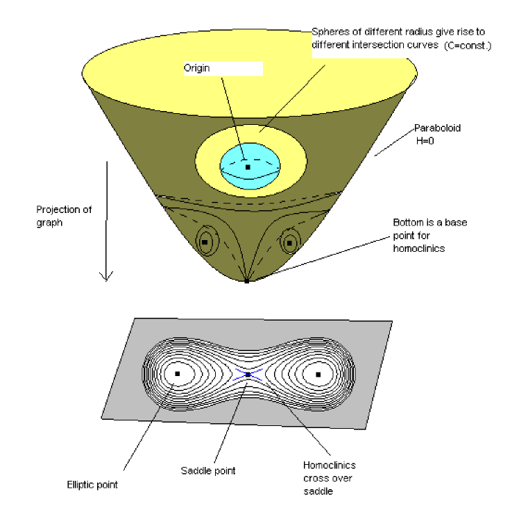
Figure 1: The intersections of the spheres $K=const.$ with the paraboloid $H=0$ and their projections to the $M_{1}M_{2}$ plane.

Figure 2: Phase portrait for the reduced equations obtained via the projection in figure 1, for $a$ = 2 , $P$ = 1, and $K$ small.

Eq. (27) yields $M_{3}$ in terms of $M_{1}$ and $M_{2}$ on the paraboloid. Plug this expression for $M_{3}$ into $K$ to find that on the paraboloid

$$K=(1-\frac{2}{9}c(a)a)M_{1}^{2}+(1-\frac{2}{9}\frac{c(a)}{a})M_{2}^{2}+\frac{1}{9}(aM_{1}^{2}+\frac{1}{a}M_{2}^{2})^{2}+c(a)^{2}.$$

For $a$ close to $1$ the coefficients of the quadratic terms, $M_{1}^{2}$ and $M_{2}^{2}$ are positive, and close to $1/2$. The only critical point for $K$ is the origin and is a nondegenerate minimum. It follows from a basic argument in Morse theory that all the intersection curves are closed curves, circling the origin. As $a$ increases the sign of the coefficient in front of the $M_{1}^{2}$ term eventually crosses $0$ and becomes negative. This happens when $1-\frac{2}{9}c(a)a=0$ which works out to $a=\sqrt{3}$. After that the origin becomes a saddle point for $K$, and the level set of $K$ passing through the origin has the shape of a figure 8, with the cross at the origin. Inside each lobe of the eight is a new critical point. See figure 2 below. This change as $a$ crosses past $\sqrt{3}$ is an instance of what is known as a “Hamiltonian pitchfork bifurcation” or “Hamiltonian figure eight” bifurcation among specialists in Hamiltonian bifurcation theory.

To re-iterate: for $1<a<\sqrt{3}$ all reduced solution curves are closed and surround the origin. For $a>\sqrt{3}$ the origin becomes a saddle point, and the level set of $K$ passing through the origin consists of three solution curves: the origin itself which is now an unstable equilibrium, and two homoclinic orbits corresponding to the two lobes of the eight. Being homoclinic to the unstable equilibrium, it takes an infinite time to traverse either one of these homoclinic lobes.

The situation is symmetric as $a$ decreases, with the bifurcation occurring at $a=1/\sqrt{3}$. This is as it must be, from the discrete symmetry alluded to in Proposition 2.1, $a\mapsto 1/a$, $M_{1}\mapsto M_{2},M_{2}\mapsto M_{1}$.

7 Step 4: Berry phase and unreducing.

As per the discussion in (5.2.4), associated to each choice of closed solution curve $C\subset\mathbb{R}^{3}\times\{1\}$ and each choice $\mu\neq 0$ of momentum, we have a family of chains which lie on a fixed two torus $T^{2}=T^{2}(C;\mu)\subset T^{*}S^{3}$. Our question is : are the chains on this $T^{2}$ closed? The Fefferman dynamics restricted to $T^{2}$ is that of linear flow on a torus. Let $\phi$ be a choice of angular variable around $C$, which we call the base angle. Let $\theta$ be the other angle of the torus, which we call the ‘vertical angle’ chosen so that the projection $T^{2}\to C$ is $(\phi,\theta)\mapsto\phi$. We take both angles defined mod $2\pi$. As we traverse the chain, every time that the base angle $\phi$ varies from $0$ to $2\pi$, (which is to say we travel once around $C$) the vertical angle $\theta$ will have varied by some amount $\Delta\theta$. The amount $\Delta\theta$ does not depend on the choice of chain within $T^{2}$. If $\Delta\theta$ is a rational multiple of $2\pi$ then the chains in $T^{2}$ are all closed. If $\Delta\theta$ is an irrational multiple of $2\pi$, then none of the chains in $T^{2}$ close up, and we have the case of quasi-periodic chains corresponding to irrational flow on $T^{2}$.

Without loss of generality we can suppose that $\mu=r_{0}e_{3}$ where $e_{3}$ denotes the final element of the standard basis of $su(2)^{*}=\mathbb{R}^{3}$. For why we can assume this without loss of generality refer to subsection 5.2.3 above. In this case $K=r_{0}^{2}$ and this fixing of $K$almost fixes the reduced curve $C$. (See the second paragraph in the proof of the proposition immediately below for details.) Remembering the modulus parameter $a$, we see that

$$\Delta\theta=\Delta\theta(K,a).$$

Since the dynamical system defined by the Fefferman metric depends analytically on initial conditions and on the parameter $a$, we see that $\Delta\theta(K,a)$ is an analytic function of $a$ and $K$. It follows that in order to prove theorem 1, all we need to do is show that for a single value of $a$, the function $K\mapsto\Delta\theta(K,a)$ is non-constant. We see that in order to prove Theorem 1 it only remains to prove:

Proposition 7.1

For $a>\sqrt{3}$ the function $K\mapsto\Delta\theta(K,a)$ is non-constant.

Proof of Proposition.

Fix $a>\sqrt{3}$. Consider the value $K=c(a)^{2}$ corresponding to the homoclinic figure eight through the origin in the $M_{1}M_{2}$ plane. We will show that

$$\lim_{K\to c(a)^{2}_{-}}\Delta\theta(K,a)=+\infty.$$ (28)

and that for $K$ slightly less than $c(a)^{2}$ the value of $\Delta\theta(K,a)$ is finite. It follows that the function $K\mapsto\Delta\theta(K,a)$ varies, as required.

Let $m(a)$ denote the absolute minimum of $K$ on the paraboloid. The minimum is achieved at two points, the elliptic fixed points inside each lobe of the homoclinic eight. For values of $r_{0}^{2}$ between $m(a)$ and $c(a)^{2}$ the level set $K=r_{0}^{2}$ consists of two disjoint closed curves $C_{1},C_{2}$, one inside each lobe of the eight. These two curves are related by the reflection $(M_{1},M_{2})\mapsto(-M_{1},M_{2})$. The entire dynamics is invariant under this reflection, so that the value of $\Delta\theta$ on $C_{1}$ equals its value on $C_{2}$. (The two components are traversed in the same sense.) Consequently $\Delta\theta(K,a)$ is well-defined and finite for $m(a)<K<c(a)^{2}$, being equal to the common value of $\Delta\theta(C_{i})$.

In what follows we arbitrarily fix one of the two components of $K=r_{0}^{2}$ and call it $C$.

The key to establishing the limit (28) is a Berry phase formula for $\Delta\theta$ which mimics earlier work of one of us ([14]). The formula expresses $\Delta\theta$ as the sum of two integrals:

$$\Delta\theta(K,a)=\hbox{dynamic}+\hbox{ geometric }$$ (29)

where

$$\hbox{ dynamic }={1\over{\sqrt{K}}}\int_{0}^{T}fdt$$

and

$$\hbox{ geometric}=-(\hbox{oriented solid angle}).$$

Both the dynamic and the geometric terms can be expressed as line integrals around $C$. In the dynamic term, $T=T(K)$ is the period of the curve $C$, and where

$$f=\frac{1}{2}[aM_{1}(t)^{2}+\frac{1}{a}M_{2}(t)^{2}+c(a)].$$ (30)

The integral is done around the projection of the curve $C$ to the $M_{1}M_{2}$. The time $t$ is the time parameter occuring in the reduced equations, which is the same as the geodesic time. In the second formula, the oriented solid angle is the standard oriented solid angle enclosed by a closed curve such as $C$ in space. The absolute value of an oriented solid angle is always bounded by $4\pi$. On the other hand, $\frac{1}{\sqrt{K}}f>\frac{1}{2\sqrt{K}}c(a)$. Consequently, if we let the curve $C$ approach the lobe of the homoclinic orbit which contains it, then its period $T(K)$ tends to $\infty$. We now see that the dynamic term of eq. (29) tends to $+\infty$. Thus, the corollary is proved once we have established the validity of the Berry phase type formula (29).

7.1 Proof of Berry phase formula

We begin the proof of eq. (29) by recalling and summarizing our situation, and applying the discussion of (5.2.4) for relating the reduced dynamics to dynamics in $T^{*}(SU(2)\times S^{1})$ and curves in $T^{*}SU(2)$. We have fixed $J=(L,P)$ to equal the value $\mu=(r_{0}e_{3},1)\in R^{3}\times\mathbb{R}$ where $r_{0}\neq 0$. The values of the Casimirs which characterize our reduced curve $C$ are then $K=r_{0}^{2}$, and $P=1$. The Fefferman light-like geodesics $C_{F}$ associated to $C$ and our choice of $\mu$ must lie on the manifold $J^{-1}(\mu)\cap\pi^{-1}(C)$ which is a three-torus inside $T^{*}(SU(2)\times S^{1})$. Project this three torus into $T^{*}S^{3}$ via the product structure induced projection: $pr_{2}:T^{*}(S^{3}\times S^{1})=T^{*}S^{3}\times T^{*}S^{1}\to T^{*}S^{3}$ and in this way arrive at a two-torus $X(C)=pr_{2}(J^{-1}(\mu))\cap\pi^{-1}(C)\subset T^{*}SU(2)\times\{1\}$ which projects onto $C$ via the canonical projection $T^{*}(SU(2))\times\{1\}\to\mathbb{R}^{3}\times\{1\}$. We will soon need that $X(C)\subset L^{-1}(r_{0}e_{3})\times\{1\}$ which follows from the fact that $J=(L,P)$ so that $pr_{2}(J^{-1}(\mu))=L^{-1}(r_{0}e_{3})\times\{1\}$. The canonical projection just refered to is that of the quotient map $T^{*}(SU(2))\to\mathbb{R}^{3}$ for the (lifted) left action of $SU(2)$ on itself. The momentum map associated to this map is $L$. We will also use that the canonical projection, $T^{*}(SU(2))\to\mathbb{R}^{3}$, restricted to level sets of $L$, corresponds to symplectic reduction for $T^{*}SU(2)$. The chains $ch$ associated to the reduced solution $C$ and our choice of momentum axis $e_{3}$ lie in the two-torus $X(C)$. To coordinatize $X(C)$ choose any global section $\hat{C}:C\to X(C)$ and let $\phi$ be an angular coordinate around $C$ so that $\hat{C}$ is a closed curve in $X(C)$ parameterized by $\phi$ and projecting onto $C$. Now act on $\hat{C}$ by the one-parameter subgroup $exp(\theta e_{3})=SU(2)_{L}$. Then any point of $X(C)$ can be written as $exp(\theta e_{3})\cdot\hat{C}(\phi)\in X(C)$ where $\theta,\phi$ are global angular coordinates. (The multiplication “$\cdot$” of “$exp(\theta e_{3})\cdot\hat{C}(\phi)$” denotes the action of the group element $exp(\theta e_{3})\in SU(2)$ on $T^{*}SU(2)$ by cotangent lift.)

Every cotangent bundle $T^{*}Q$ is endowed with a canonical one-form. Let $\Theta$ be the canonical one-form on $T^{*}SU(2)$. Our Berry phase formula (29) will be proved by applying Stoke’s theorem to the integral of $\Theta$ around a well-chosen closed curve $c$ in $X(C)$.

This curve $c\subset X(C)\subset T^{*}SU(2)\times\{1\}$ is the concatenation of two curves. One curve is any one of the chains $ch$ corresponding to $C$ – which is to say, the projection by $pr_{2}$ of any one of the Fefferman geodesics $C_{F}\subset J^{-1}(\mu)\cap\pi^{-1}(C)$. We parameterize $ch$ by the Fefferman dynamical time, $0\leq t\leq T$ making sure to stop when, upon projection,we have gone once round $C$, so that $C(0)=C(T)$. Having gone once round $C$, we must have $ch(T)=exp(\Delta\theta e_{3})\cdot c(0)$. The holonomy $\Delta\theta$ is the angle we are trying to compute. For the other curve $c_{group}$ we simply move backwards in the group direction to close up the curve: $c_{group}(s)=exp(-se_{3})\cdot ch(T)$. Our curve $c$ is then the concatenation $+$ of these two smooth curves:

$$c=c_{group}+ch.$$

The curve $c$ is a closed curve lying in the two-torus $X(C)$. Not all closed curves in the two-torus bound discs, but $X(C)\subset L^{-1}(r_{0}e_{3})\times\{1\}\cong SU(2)$ which is simply connected, so that $c$ does bound a disc $\tilde{D}\subset L^{-1}(r_{0}e_{3})\times\{1\}$. Apply Stoke’s formula:

$$\int_{\tilde{D}}d\Theta=\int_{c_{group}}\Theta+\int_{ch}\Theta.$$ (31)

The proof of (29) proceeds by evaluating each term in eq (31) separately.

Write $S^{2}$ for the two-sphere $K=r_{0}^{2}$, $P=1$. Write $\pi_{r_{0}}:L^{-1}(r_{0}e_{3})\to S^{2}$ for the restriction of the canonical reduction map $\pi:T^{*}SU(2)\times\{P=1\}\to\mathbb{R}^{3}\times\{1\}$. Under $\pi_{r_{0}}$ the disc $\tilde{D}$ projects onto a topological disc $D\subset S^{2}$ which bounds our reduced curve $C$. $S^{2}$ is the symplectic reduced space of $T^{*}SU(2)$ by the left action of $SU(2)$, reduced at the value $L=r_{0}e_{3}$. A basic result from symplectic reduction, essentially its definition, asserts that as a symplectic reduced space $S^{2}$ is endowed with a 2-form $\omega_{r_{0}}$ (the reduced symplectic form) defined by $\pi_{r_{0}}^{*}\omega_{r_{0}}=i^{*}(-d\Theta)$, where $i:L^{-1}(r_{0}e_{3})\to T^{*}SU(2)$ is the inclusion. Let $d\Omega$ denote the unique rotationally invariant two-form on the two sphere, normalized so that its integral over the entire sphere is $4\pi$. (The form $d\Omega$ is not closed, but the notation is standard, and suggestively helpful, so we use it.) It is well-known that $\omega_{r_{0}}=-r_{0}d\Omega$, which is to say, that

$$r_{0}(\pi_{r_{0}}^{*}(d\Omega))=i_{r_{0}}^{*}(d\Theta).$$

(See [1] for the standard “high-tech” computation, and [14] for an elementary computation of this well-known fact.) Thus

$$\int_{\tilde{D}}(d\Theta)=\int_{D}r_{0}d\Omega=r_{0}(\hbox{ solid angle enclosed by }C)$$ (32)

It is worth noting that this area is a signed area, positive or negative depending on the orientation of the bounding curve $C$ of $D$.

It follows from the definition of the momentum map on the cotangent bundle that $\Theta({d\over{ds}}(exp(se_{3})(p))=r_{0}$ for any point $p\in L^{-1}(r_{0}e_{3})$. It follows that

$$\Theta=r_{0}d\theta\hbox{ along }c_{group},$$

and thus

$$\int_{c_{group}}\Theta=-r_{0}\Delta\theta.$$ (33)

where the minus sign arises because in travelling along $c_{group}$ we moved backwards in the $e_{3}$-direction.

It remains to compute $\int_{ch}\Theta$. For this computation we will have to work on $T^{*}(SU(2)\times S^{1})$. There we have the canonical one form

$$\Theta_{F}=\Theta+Pd\gamma.$$ (34)

Now relative to any coordinates $x^{a}$ for $SU(2)\times S^{1}$, where $p_{a}$ are the corresponding momentum coordinates we have

$$\Theta_{F}=\Sigma p_{a}dx^{a}.$$

Plugging in along one of the light-like Fefferman geodesics and using the metric relation $p_{a}=\Sigma g_{ab}\dot{x}^{a}$ where $g_{ab}$ are the metric components we see that

$$\Theta_{F}(\dot{C}_{F}(t))=2H=0$$

where the last equality arises because the Fefferman geodesic is light-like. Since $pr_{2}\circ C_{F}=ch$ where $pr_{2}:T^{*}SU(2)\times T^{*}S^{1}\to T^{*}SU(2)$ is the projection, we have, from (34),

$$\Theta({d\over{dt}}ch)=-P\dot{\gamma}=-\dot{\gamma},$$

where we used $P=1$. It follows that

$$\int_{ch}\Theta=-\int_{0}^{T}\dot{\gamma}dt$$

. Now $\dot{\gamma}=\frac{\partial H}{\partial P}$. Referring back to the equation for the Hamiltonian, and remembering that we set $P=1$ after differentiating we see that

$$\dot{\gamma}=-\frac{3}{2}M_{3}-c(a).$$

Now using the formula for $M_{3}$ in terms of $M_{1},M_{2}$ and a bit of algebra we see that

$$-\dot{\gamma}=f,$$

where $f$ is as in the eq. (30). Thus:

$$\int_{ch}\Theta=\int_{0}^{T}fdt.$$ (35)

Putting together the pieces (32), (33), (35) into Stokes’ formula (31) and some algebra yields the Berry phase formula (29). QED

APPENDICES

Appendix A The dynamics when $a=1$.

The chains for the standard structure on $S^{3}$ are formed by intersecting $S^{3}\subset\mathbb{C}^{2}$ with complex lines in $\mathbb{C}^{2}$. See [10]. In this appendix we verify that the Fefferman metric description of chains when $a=1$ yields these circles.

The key to our verification is the observation that when $a=1$ the Fefferman Hamiltonian (26) splits into two commuting pieces $H=H_{0}-H_{1}$ with $\{H_{0},H_{1}\}=0$. This observation and the following method of computation is the same one which led to explicit formulae for subRiemannian geodesic flows in chapter 11 of [13], formulae identical to that of Lemma 1 below. We have $H_{0}={1\over 2}K={1\over 2}(M_{1}^{2}+M_{2}^{2}+M_{3}^{2})$ and $H_{1}=\frac{1}{2}(M_{3}-\frac{3}{2}P)^{2}$. Since the two Hamiltonians commute, their flows up on the cotangent bundles commute. This observation leads to the explicit formula for the chains through the identity:

$$ch(t)=exp\left[t(M_{1}e_{1}+M_{2}e_{2}+M_{3}e_{3})\right]exp\left[-t(M_{3}-\frac{3}{2}P)e_{3})\right]$$ (36)

The $M_{i},P$ are constants which satisfy the $H=0$ condition

$$(M_{1}^{2}+M_{2}^{2}+M_{3}^{2})=(M_{3}-\frac{3}{2}P)^{2}.$$

In this formula (36) for the chains, the first factor corresponds to the flow of $H_{0}$, whose integral curves correspond to one-parameter subgroups in $SU(2)$, and the second factor corresponds to the projection to $SU(2)$ of solutions to the Hamilton’s equation for $-H_{1}$.

To verify that the chains computed via Fefferman’s metric are the circles described above we use two lemmas from linear algebra.

Lemma 1. ( circles in SU(2)) Every geometric circle in $SU(2)=S^{3}$ through the identity can be parameterized as $\gamma(t)=exp(\alpha t)exp(-\beta t)$ where $\alpha,\beta\in su(2)$ are Lie algebra elements of the same length.

Lemma 2. When $\beta=ce_{3}$ as in eq. (36) then these circles sit on complex lines.

Remark. The condition $|\alpha|=|\beta|$ in lemma 1 is a $1:1$ resonance condition.

The proofs rely on identifying the quaternions $\mathbb{H}$ with $\mathbb{C}^{2}$ and hence the group of unit quaternions with $SU(2)$ and $S^{3}$. Since the contact plane is annihilated by $\omega_{3}$, and is to correspond with the $T_{x}S^{3}\cap\mathbb{J}T_{x}S^{3}$, we must take the identification $\mathbb{C}^{2}\cong\mathbb{H}^{2}$ such that the complex structure on $\mathbb{C}^{2}$ corresponds to right multiplication by $k$, where $k$ is to correspond to $e_{3}$ in $su(2)$.

Proof of lemma 1. In a Euclidean vector space, (such as $\mathbb{H}$) the circles are described by $c(t)=P+r(\cos(\omega t)e_{1}+\sin(\omega t)e_{2})$ where $P$ is the center of the circle, $r$ its radius, and where $e_{1},e_{2}$ are an orthonormal basis for the plane through $P$ containing the circle. Now use the fact that for a unit quaternion $n$ we have $exp(nt)=\cos(t)1+\sin(t)n$. Thus $\gamma(t)$ of lemma 1 is equal to $(\cos(t)+\sin(t)\alpha)(\cos(t)-\sin(t)\beta)$. Algebra and trigonometry identities yield

$$\gamma(t)=\frac{1}{2}[(1-\alpha\beta)+\cos(2t)(1+\alpha\beta)+\sin(2t)(\alpha-\beta)]$$

which we can rewrite as

$$\gamma(t)=P+\cos(2t)v+\sin(2t)w,$$

with $P=\frac{1}{2}(1-\alpha\beta)$, $v=\frac{1}{2}(1+\alpha\beta)$ and $w=\frac{1}{2}(\alpha-\beta)$. It remains to show that $v$ and $w$ have the same length and are orthogonal. Using $\bar{\alpha}=-\alpha$ and remembering that $\alpha$ is unit length we see that we have $v=-\alpha w$ and so indeed $|v|=|w|$. Their common length is the radius $r$ of the circle. Since the Euclidean inner product is given by $Re(v\bar{w})$ the fact that $v=-\alpha w$ also shows that $v$ and $w$ are orthogonal. QED

Proof of lemma 2. Let $v,w$ be as in the proof of lemma 1. We must show that the real 2-plane spanned by $v$ and $w$ is a complex line when $\beta=k$. Recall that under our identification of $\mathbb{C}^{2}$ with $\mathbb{H}$ the complex structure corresponds to multiplication on the right by $k$. Now compute $wk=v$, to see that the span of $v$ and $w$ is indeed a complex line. QED

Appendix B Relation to the Rossi example.

Rossi [15] constructed a much-cited example of a family of non-embeddable CR-structures on $S^{3}$. The purpose of this appendix is to show that Rossi’s family is isomorphic to our left-invariant CR family with $a\neq 1$. This isomorphism is well-known to experts. We include it here for completeness. We use the description of CR manifolds to be found in the remark towards the beginning of section 3.1. In that construction a CR structure is defined as the span of complex vector field. Let $Z$ be the complex vector field corresponding to the standard CR structure. In terms of our left invariant frame, $Z=e_{1}-ie_{2}$. Then Rossi’s perturbed CR structure is defined by

$$Z_{\mu}=Z-\mu\bar{Z}$$

with $\mu$ a real parameter. On the other hand, we saw (again, eq. 5) that our left-invariant CR structures correspond to the span of

$$Z_{a}=e_{1}-\frac{i}{a}e_{2}.$$

Set $a=1+\epsilon$ and expand out: $Z_{a}=e_{1}-i(1+\epsilon)e_{2}=e_{1}-ie_{2}-i\epsilon e_{2}=Z+\frac{1}{2}\epsilon(Z-\bar{Z})$. Upon rescaling $Z_{a}$ by dividing by $(1+\frac{1}{2}\epsilon)$ we see that $span(Z_{a})=Span(Z-\mu(\epsilon)\bar{Z}$, where $\mu(\epsilon)=\frac{\frac{1}{2}\epsilon}{1+\frac{1}{2}\epsilon}$. This shows that the left-invariant structure for $a$ corresponds to Rossi’s structure for $\mu=\mu(\epsilon)$.

The important facts concerning Rossi’s structures for $\mu\neq 0$ is that every CR-function for one of these structures on $S^{3}$ is even with respect to the antipodal map $(x,y,z)\mapsto(-x,-y,-z)$. We recommend Burns’ [3] for the proof. This forced evenness s implies that there is no CR embedding of our left-invariant structures for $a\neq 1$ into $\mathbb{C}^{n}$ for any $n$. The structures do however, have explicit $2:1$ immersions into $\mathbb{C}^{3}$ which can be found in Rossi. See also Burns ([3]) or Falbel [7]. Upon taking the quotient by the antipodal map each $a\neq 1$ structure induces a left-invariant CR structure on $\mathbb{R}P^{3}=SO(3)$ which does embed into $\mathbb{C}^{3}$. This embedded image bounds a domain within an explicit Stein manifold $S\subset\mathbb{C}^{3}$.

Open Problem. [Dan Burns] Find a synthetic construction of the chains for the left-invariant structures, in the spirit of the construction of the chains for the standard structure, but using a family of complex curves in $S$ in place of the straight lines used to construct the chains for the standard structure.

Appendix C Acknowledgements.

We would like to thank John Lee for explaining the connection between the Rossi example and the left-invariant structures as detailed in Appendix 2, and Dan Burns for e-mail conversations for further considerations concerning Appendix 2, and for the open problem, and for listening critically to an early version of our results. We would like to acknowledge encouragement and helpful conversations from Gil Bor of CIMAT, Jie Qing (UCSC), and Robin Graham (U. of Washington). We would especially like to thank Gil Bor for crucial help regarding the reduced dynamics, and CIMAT (Guanajuato, Mexico) for support during this time. The junior author also thanks AGEP for some financial aid in many instances of the project.

References

- [1] R. Abraham and J. E. Marsden, Foundations of Mechanics, Second Edition, Addison-Wesley, Boston, 1994.
- [2] V. I. Arnold, Mathematical methods of classical mechanics. Translated from the Russian by K. Vogtmann and A. Weinstein. Second edition. Graduate Texts in Mathematics, 60. Springer-Verlag, New York, 1989.
- [3] D. Burns, Global behavior of some tangential Cauchy-Riemann equations in “Partial Differential Equations and Geometry” (Proc. Conf., Park City, Utah, 1977); Dekker, New York, 1979, p. 51.
- [4] A. Cap, On left-invariant CR-structures on SU(2). Preprint arXiv:math.DG/0603730 v1.
- [5] E. Cartan, Sur la geometrie pseudo-conforme des hypersurfaces de le espace de deux variables complexes. Ann. Mat. Pura Appl., IV. Ser. 11 (1932).
- [6] S. S. Chern, J. K. Moser, J. K. “Real hypersurfaces in complex manifolds”, Acta Math. 133 (1974), 219–271.
- [7] Elisha Falbel, Non-embeddable CR-manifolds and Surface Singularities. Invent. Math. 108 (1992), No. 1, 49-65.
- [8] F. A. Farris, An Intrinsic Construction of Fefferman’s CR-metric. Pacific Journal of Mathematics, Vol.123, No.1, 1986.
- [9] C. L. Fefferman, Monge-Ampere equations, the Bergman kernel, and geometry of pseuconvex domains. Ann. of Math (2) 103 (1976), N0.2, 395-416.
- [10] W. M. Goldman, Complex Hyperbolic Geometry. The Clarendon Press, Oxford University Press, New York, 1999.
- [11] N. Hitchin, Twistor Spaces, Einstein metrics, and isomonodromic deformations, J. Diff. Geom. v. 42, no. 1, 30-112, (1995).
- [12] J. M. Lee, The Fefferman metric and pseudohermitian invariants. Trans. Amer. Math. Soc. 296 (1986), 411-429.
- [13] R. Montgomery, A tour of subriemannian geometries, their geodesics and applications. (English summary) Mathematical Surveys and Monographs, 91. American Mathematical Society, Providence, RI, 2002.
- [14] R. Montgomery, How much does the rigid body rotate? A Berry’s phase from the 18th century. Amer. J. Phys. 59 (1991), no. 5, 394–398.
- [15] H. Rossi, Attaching analytic spaces to an analytic space along a pseudoconcave boundary. 1965 Proc. Conf. Complex Analysis (Minneapolis, 1964) pp. 242–256, Springer, Berlin.