Complexity of spectral sequences: semiclassical approach

Abstract

It has been long recognized that the task of semiclassical evaluation of quantum spectra for the classically nonintegrable systems is fundamentally more complex than for the classically integrable ones. Below it is argued that the quantum spectra of the chaotic systems can differ among themselves by level of their complexity.

I Introduction

It is well known that the structure of the spectrum of a quantum mechanical system reflects the dynamical properties of its classical counterpart. The degree of classical dynamical regularity is reflected in the general statistical properties of the quantum spectra and in the nature of the analytical solution of the spectral problem.

For the conservative systems, dynamical regularity is usually understood as the possibility to specify the trajectories via a set of quantities that remain constant throughout dynamical evolution – the integrals of motion. If each one of the $d$ degrees of freedom of a bounded system corresponds to a conserved quantity, $I_{1}$, …, $I_{d}$, then such a system is completely integrable and its dynamical behavior can be regarded, in suitable coordinates, as a combination of oscillations. Algebraically, this is a manifestation of the underlying symmetries in the system, that lead to the appearance of certain global structures in the phase space known as integrable tori Arnold , that uphold the oscillatory pattern of the trajectories.

As it was pointed out by the EBK theory, in semiclassical regime the integrals of motion assume a set of discrete values, defined via the so called quantum numbers, $n_{i}$,

$$I_{i}\sim\hbar\left(n_{i}+\frac{\mu_{i}}{4}\right),$$ (1)

where $\hbar$ is the Plank’s constant and $\mu_{i}$ is the Maslov index Gutzw ; Cvit . In view of (1), each integral of motion provides a uniform global map from the natural numbers into the spectral sequence, which leads to the analytical solution to the corresponding quantum mechanical spectral problem. For example, if the energy is defined in terms of the motion integrals as $E=E^{(\mathop{\rm class})}\left(I_{1},...,I_{d}\right)$, the quantum eigenvalues of energy are

$$E^{(\mathop{\rm class})}\left(I_{1},...,I_{d}\right)\rightarrow E^{(\mathop{\rm quant})}\left(\hbar\left(n_{1}+\frac{\mu_{1}}{4}\right),...,\hbar\left(n_{d}+\frac{\mu_{d}}{4}\right)\right).$$ (2)

The integers $n_{i}$ can be interpreted as the number of times the wave representing the quantum mechanical particle winds around the basic torus cycles, so physically, the discretization of the spectrum in the EBK theory can be understood as a manifestation of the geometrical consistency between the (semiclassical) quantum waves and the dynamical trajectories.

In contrast, if the number of motion integrals is less than the number of the degrees of freedom, then the dynamics is “irregular”, in the sense that its trajectories do not follow any particular patterns in the phase space. Rather, they tend to cover as much phase space $X$ as possible at a given energy, more or less uniformly, so the only relevant long term characteristics of the dynamics are the relative frequencies of the visitations of different parts of $X$, which can be equally well described by a certain smooth probability distribution $P(x)$.

As a result, the complexity of the semiclassical quantization task for the nonintegrable systems differs substantially from the integrable ones. While the EBK quantization method is constructive, i.e. it is possible to define the individual levels of the quantized integrable systems explicitly, by specifying a particular set of quantum numbers (2), for nonintegrable systems such individualized solution for the spectral problem is generally unavailable. Instead, one of the main results of the semiclassical theory is the series expansion representation for the quantum density of states, which is a global characteristics of the spectrum, the so-called Gutzwiller’s formula:

$$\rho(E)=\sum_{n}\delta\left(E-E_{n}\right)=\bar{\rho}(E)+\mathop{\rm Re}\sum_{p}B_{p}(E)e^{iS_{p}(E)}.$$ (3)

Here $S_{p}(E)$ is the action functional evaluated for the periodic orbit $p$, and $B_{p}$ is a certain weight factor Gutzw .

One can immediately appreciate the difference in complexity of the series (3) compared to the (2). The sum (3) includes all the periodic orbits (that are isolated in a fully chaotic system), and so it reflects the full complexity of the classical phase space structure of a nonintegrable system. The essence of the Gutzwiller’s formula is that the oscillating amplitudes $e^{iS_{p}(E)}$ produced by the periodic orbits, combined with the appropriate weights $B_{p}$, produce a constructive interference effect every time $E$ happens to be equal to one of the quantum eigenvalues and cancel each other out for all other values of $E$, which enables one to transform the information contained phase space structures into the pattern of quantum mechanical spectral sequence Gutzw .

An important aspect of (3) is that it is indeed a very general result, that can be applied to a great variety of systems. Moreover, certain mathematical systems or objects can be put into a quantum chaotic context because their constituents can be related via formula (3) and hence be interpreted as “quantum chaotic”. One well known example of this is provided by the relationship between the eigenvalues of the Laplace - Beltrami operator on a surface of constant negative curvature and the dynamics of a point particle moving on it. This connection is described by the famous Selberg trace formula Selberg , that was first discovered as a number theoretic and functional analysis theorem. Apart from the deterministic chaotic systems, the expansion (3) can also describe the spectra of many classically stochastic systems, e.g. the so-called quantum graphs QGT ; Gaspard and 2D ray splitting billiards Blumel : as long as the stochastic dynamics generates trajectory patterns similar to the deterministic chaotic trajectories, they manifest themselves in the in the same physical context in quantum regime.

Perhaps the most intriguing example is provided by the relationship between the zeroes of Riemann’s zeta function and the set of the prime numbers. In Berry1 ; Berry3 ; Berry4 it was argued that the integrated spectral density, the spectral staircase of the imaginary parts of the nontrivial zeroes of Riemann’s zeta function, $E_{n}=\mathop{\rm Im}(z_{n})$, $\zeta(z_{n})=0$,

$$N(E)=\sum_{n}\Theta\left(E-E_{n}\right)$$ (4)

can be expanded into the Gutzwiller type series (3) in which the average part of the density of $E_{n}$s is given by

$$\bar{N}(E)=\frac{E}{2\pi}\left(\ln\left(\frac{E}{2\pi}\right)-1\right)+\frac{7}{8}+...,$$ (5)

and the oscillating part by

$$\delta N(E)\approx-\frac{1}{\pi}\mathop{\rm Im}\sum_{p}\sum_{m=1}^{\infty}\frac{e^{imE\ln p}}{mp^{\frac{m}{2}}},$$ (6)

where the index $p$ runs over the set of prime numbers. Hence the prime numbers in this case play the role of the prime periodic orbits of lengths $L_{p}=\ln p$. This shows that the organization of the roots of the zeta function, which a is purely number theoretic object, is as irregular with respect to the set of prime numbers, as is the quantum spectrum of a classically chaotic system as expressed by the “periodic orbit expansion” Bogomolny2 ; Cvit .

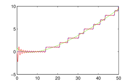
Figure 1: Spectral staircase for the imaginary parts of zeroes of Riemann’s zeta function. Wiggly line represents the Gutzwiller’s series for $N(k)$, and the smooth line running through the staircase is the Weyl’s average $\bar{N}(k)$.

Despite these significant implications of Gutzwiller’s formula, it does not produce the final solution of the spectral problem in the same sense as the EBK theory does for the integrable systems. The problem is that the Gutzwiller’s formula does not specify the individual energy or momentum eigenvalues, i.e. it does not produce a functional correspondence between the spectral sequence and the natural number (quantum number) sequence, although such correspondence actually can exist.

In order to evaluate the individual eigenvalues $E_{n}$ from (3), one needs to provide additional local information, that would allow to single out the individual delta peaks in $\rho(E)$. To have a uniform solution to the spectral problem that would be equivalent to the EBK formula (2), one must be able to produce such information systematically, in a way that would eventually lead to an explicit functional dependence $E_{n}=E(n)$.

It is easy to show that in principle this not an impossible task. Indeed, consider a the spectral staircase (4), that monotonously increases with energy. Consider also a smooth monotone function $f(E)$ that intersects every stair step of $N(E)$ as shown on Fig. 2.

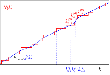
Figure 2: Spectral staircase $N(k)$ for the eigenvalues of momenta of quasi one dimensional quantum networks (quantum graphs), that are known to be stochastic in classical limit (see. Section III). A smooth monotone function $f(k)$ intersects every stair-step of $N(k)$.

It is also possible to chose $f(E)$ in such a way that the average deviation of $f(E)$ from $N(E)$ vanishes, $\left\langle f(E)-N(E)\right\rangle=0$, so $f(E)$ can be considered as an “average” of $N(E)$, that is in general different from the Weyl’s’ average Baltes . The intersection points $\hat{E}_{n}$, $f\left(\hat{E}_{n}\right)=N\left(\hat{E}_{n}\right)=n$, satisfy the condition

$$...\leqslant E_{n-1}\leqslant\hat{E}_{n}\leqslant E_{n}\leqslant\hat{E}_{n+1}\leqslant E_{n+1}\leqslant...\ .$$ (7)

Since $f(E)$ is monotone, it can be inverted, so the roots of $f(\hat{E}_{n})=N\left(\hat{E}_{n}\right)$, can be defined as a function of $n$, $\hat{E}_{n}=f^{-1}(n)=\hat{E}(n)$. The resulting separating sequence (7) can then be used to find the eigenvalues $E_{n}$ in the form of an explicit formula Opus ; Prima ; Sutra ; Stanza ,

$$E_{n}=E(n)=\int_{\hat{E}(n-1)}^{\hat{E}(n)}\rho(E^{\prime})E^{\prime}dE^{\prime}.$$ (8)

Due to the expansion (3), one can in principle evaluate the integral (8) explicitly and obtain the formula for $E_{n}=E(n)$ in an expansion form structurally similar to (3). In general, the structure of the classical phase space and hence the structure of the sum (3) can change in very complex ways as a function of energy, which makes the evaluation of the integral (8) a much more complicated problem. In order to avoid these difficulties, the following discussion will be restricted to the so-called scaling systems, e.g. the billiards, in which case the expansion coefficients $B_{p}$ are energy independent and the functional structure of the periodic orbit sum (3) is fixed.

Such construction produces a map from the natural number sequence first into the separating sequence $\hat{E}_{n}=f^{-1}(n)$, and then to physical spectral sequence $E_{n}$ via (8). Hence in fully nonintegrable system there also exists a solution to the spectral problem that produces the eigenvalues $E_{n}$ as a function of $n$, $E_{n}=E(n)$ based on the semiclassical expansion (3).

Formulae (7) and (8) suggest that the possibility to solve the spectral problem depends on the possibility to localize the individual delta peaks within intervals $I_{n}=\left[\hat{E}_{n},\hat{E}_{n-1}\right]$, loosely defined by the inequality (7). From such perspective, the missing part of the solution is the information about the structural complexity if the spectral sequence.

II Structural analysis

The task of obtaining $\hat{E}_{n}$ is in fact much more complicated than it may appear at the first sight. Finding a monotone function that would follow the pattern of $N(k)$ in the detail required by (7) for a generic system proves to be an extremely difficult problem Baltes . As a result, outside of a few simple systems Opus ; Prima ; Sutra ; Stanza ; Saga ; Anima ; Fabula , there are virtually no examples of explicit functional dependencies of the quantum energy levels, $E_{n}$, on the index $n$, $E=E(n)$, for the classically nonintegrable systems.

The apparent impenetrability of the spectral problem for quantum chaotic systems seems to impose an implicit (and false) empirical dichotomy – either the system is integrable and explicitly quantizable via EBK theory, or it is nonintegrable and the spectral problem does not have an explicit solution. However, as it was argued above, even for a completely nonintegrable systems it is still possible to find the semiclassical solution to the spectral problem, $E_{n}=E(n)$. Moreover, the intricacy of the quantum chaotic spectra may conceal a rich complexity structure, that can be studied both within the paradigm of semiclassical physics and outside of it.

In itself, the mathematical problem is to describe the complexity of mapping the natural numbers $n=1$, $2$, … into the spectral sequence $E_{n}=E(n)$. However, in the specific context of quantum chaos theory, the task is to do this within the paradigm of the semiclassical physics, in which the objects and the phenomena of the classical dynamics provide the semantics for describing quantum objects and phenomena. The question is then, how uniform the description of spectra may be from the point of view of algorithmic complexity?

It is clear that a priori, the regularity of the delta peak patterns in $\rho(k)$ may be different for different quantum chaotic systems, so the effort required for establishing a mapping from the natural numbers into the the sequence of $\hat{E}_{n}$’s (and hence into the $E_{n}$’s) may be different, so the semiclassical solutions of spectral problems for the nonintegrable systems may not be algorithmically equivalent.

Let us examine the regularity of the spectral sequences more closely. Let $\bar{N}(E)$ be the average number of the spectral points on the interval $[0,E]$, so that $N(E)=\bar{N}(E)+\delta N(E)$, $\left\langle\delta N(E)\right\rangle=0$. For example, $\bar{N}(E)$ can be the Weyl’s average, given by the volume of the phase space of the system for the corresponding $E$. This function can be used to define the unfolded spectral sequence

$$k_{n}^{(0)}=\bar{N}(E_{n}),$$ (9)

distributed with uniform average density $\bar{\rho}^{(0)}(k)=1$, so that

$$k_{n}^{(0)}=n+\delta_{n}^{(0)},$$ (10)

with $\left\langle\delta_{n}^{(0)}\right\rangle=0$. This unfolding operation provides a common ground for studying spectral sequences coming from different systems.

Clearly, the possibility to find an analytically defined bootstrapping sequence depends on the magnitude of the fluctuations $\delta_{n}^{(0)}$. In the simplest case, if the disorder of the original sequence $k_{n}^{(0)}$ is weak, so that it is sufficiently close to a periodic sequence, then the periodic points

$$k_{n}^{(1)}=k^{(\mathop{\rm reg})}=n+\gamma^{(\mathop{\rm reg})},$$ (11)

where $\gamma^{(\mathop{\rm reg})}$ is a constant, can be interlaced with it according to (7). Geometrically, this case corresponds to the situation when the spectral staircase $N(k)$ of the unfolded sequence can be pierced by the straight line average $\bar{N}(k)$.

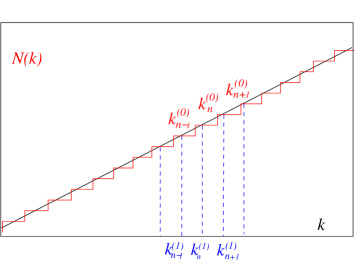
Figure 3: Spectral staircase for unfolded regular spectral sequence. Every stair-step of $N(k)$ is pierced by a single line.

The systems with such “almost integrable” spectral behavior were referred to as regular in Opus ; Prima ; Sutra ; Stanza . The numerical values for $k_{n}^{(0)}$ in this case can be computed explicitly given the explicit expansion of $\rho(k)$, via

$$k_{n}^{(0)}=\int_{n-1+\gamma^{(1)}}^{n+\gamma^{(1)}}k\rho^{(0)}(k)dk.$$ (12)

It is clear that a priori, the stair steps of a generic sequence’s staircase can not all be pierced by a single straight line, so a single periodic sequence that bootstraps the spectrum does not exist. In other words, a generic sequence $k_{n}^{(0)}$ is so disordered, that any sequence $k_{n}^{(1)}$ that bootstraps it cannot itself be periodic. Instead, the bootstrapping requires a smooth monotone curve $f(k)$ that intersects each stair-step of the spectral staircase $N(k)$ and generates a certain aperiodic sequence $k_{n}^{(1)}$ that is circumscribed in $k_{n}^{(0)}$, as shown on Fig. 2.

On the other hand, it is clear that if the bootstrapping function $f(k)$ envelops the staircase $N(k)$ maximally smoothly and uniformly, so that $\left\langle f(k)-N(k)\right\rangle=0$, then the sequence $k_{n}^{(1)}$ is more ordered than $k_{n}^{(0)}$. Since $k_{n}^{(1)}$ is more ordered than $k_{n}^{(0)}$, it may happen that $k_{n}^{(1)}$ itself can be bootstrapped by a periodic sequence, in which case $k_{n}^{(0)}$ will be bootstrapped with the periodic sequence $k_{n}^{(\mathop{\rm reg})}=n+\gamma^{(\mathop{\rm reg})}$ in two steps, via one auxiliary sequence $k_{n}^{(1)}$. If however, the $k_{n}^{(2)}$ sequence that bootstraps $k_{n}^{(1)}$ must necessarily be aperiodic, then the question will be whether the sequence $k_{n}^{(3)}$ can be chosen periodic, an so on.

This immediately suggests a clear strategy of “unfolding” any sequence $k_{n}^{(0)}$ using an auxiliary set of bootstrapped sequences $k_{n}^{(1)}$, $k_{n}^{(2)}$, …, $k_{n}^{(\mathop{\rm reg})}$,

$$k_{n}^{(0)} \leqslant k_{n}^{(1)}\leqslant k_{n+1}^{(0)},$$ (13)

$$k_{n}^{(1)} \leqslant k_{n}^{(2)}\leqslant k_{n+1}^{(1)}$$

$$...$$

$$k_{n}^{(r-1)} \leqslant k_{n}^{(r)}\leqslant k_{n+1}^{(r-1)},$$

that starts with the original sequence $k_{n}^{(0)}$ and terminates when the last sequence $k_{n}^{(r)}$ can be interlaced by a periodic sequence (11), $...\leqslant n-1+\gamma^{(\mathop{\rm reg})}\leqslant k_{n}^{(r)}\leqslant n+\gamma^{(\mathop{\rm reg})}\leqslant k_{n+1}^{(r)}\leqslant n+1+\gamma^{\left(reg\right)}\leqslant...\$. At each step, the auxiliary sequences are chosen in such a way that the size of the fluctuations $\delta_{n}^{(j+1)}=\left(k_{n}^{(j)}-n\right)$ decreases with the increase of the index $j$, so starting from the original sequence $k_{n}^{(0)}$, each following sequence is closer to periodic.

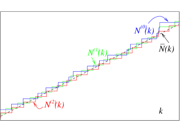
Figure 4: Bootstrapped spectral staircase $N^{(0)}(k)$s and 2 auxiliary sequences, $N^{(1)}(k)$ and $N^{(2)}(k)$ obtained for the quantum momentum spectrum of a fully connected 4-vertex quantum network. The regular staircase is pierced by the line $\bar{N}(k)$.

Let $\rho^{(j)}(k)$ be the density of the separating points at the level $j$, so $N^{(j)}(k)$ is the spectral staircase for the points $k_{n}^{(j)}$. Then the values in two bootstrapped sequences can be related to one another according to

$$k_{n}^{(j-1)}=\int_{k_{n-1}^{(j)}}^{k_{n}^{(j)}}k^{\prime}dN^{(j-1)}(k^{\prime}).$$ (14)

If the harmonic expansion similar to (3) is known for each sequence $k_{n}^{(j)}$,

$$N^{(j)}(k)=\bar{N}(k)+\mathop{\rm Im}\sum_{p}A_{p}^{(j)}e^{iS_{p}^{(j)}(k)},$$ (15)

with explicitly defined $A_{p}^{(j)}$ and $S_{p}^{(j)}(k)$ QGT ; Nova ; HBohr ; Corduneanu ; Besicovitch , then the integral (14) can be evaluated explicitly, and so the sequence $k_{n}^{(j)}$ is explicitly mapped onto $k_{n}^{(j-1)}$. Due to the mappings (14) the index $n$ propagates through the hierarchy of bootstrapped sequences (13) and emerges in the $0$th sequence $k_{n}^{(0)}$. The number of auxiliary sequences required for bootstrapping $k_{n}^{(0)}$ with $k_{n}^{(r)}$ therefore produces a certain complexity index for the quantum spectra that shows how a global index $n$ can be consistently mapped onto the spectral sequence of any degree of disorder.

There are certainly many ways in which a given sequence $k_{n}^{(j)}$ can be bootstrapped. The number of levels in the hierarchy depends on the choice of the algorithm for obtaining the bootstrapping sequences $k_{n}^{(j)}$. Given a strategy for generating the bootstrapping sequences, the regularity of the sequence can be determined empirically, either by parsing through its individual elements or by studying the probability of occurrence of the fluctuation magnitudes. In general, a separating sequence for $k_{n}^{(j)}$ can be written as

$$k_{n}^{(j+1)}=\alpha_{n}^{(j)}k_{n+1}^{(j)}+\left(1-\alpha_{n}^{(j)}\right)k_{n}^{(j)},$$ (16)

where $0<\alpha_{n}^{(j)}<1$ are arbitrary parameters. To minimize the deviation from a periodic sequence, one can consider the functional

$$F=\sum\limits_{n}\left(\left(k_{n}^{(j+1)}-k_{n-1}^{(j+1)}\right)-T\right)^{2}=\sum\limits_{n}\left(\left(\alpha_{n}^{(j)}s_{n}^{(j)}+\left(1-\alpha_{n-1}^{(j)}\right)s_{n-1}^{(j)}\right)-T\right)^{2},$$ (17)

where, for the fully unfolded sequences, $s_{n}^{(j)}=\left(1+\delta_{n+1}^{(j)}-\delta_{n}^{(j)}\right)$ and $T=1$. Varying $F$ with respect to parameters $\alpha_{n}^{(j)}$ under the conditions $0\leqslant\alpha_{n}^{(j)}\leqslant 1$ and $k_{n}^{(j+1)}>k_{n-1}^{(j+1)}$, one gets

$$\alpha_{n}^{(j)}=\frac{1}{s_{n}^{(j)}}\left(\delta_{0}^{(j)}-\delta_{n}^{(j)}\right)$$ (18)

if $0\leqslant\alpha_{n}^{(j)}\leqslant 1$, and $\alpha_{n}^{(j)}=0$ if $\alpha_{n}^{(j)}\leqslant 0$ and $\alpha_{n}^{(j)}=1$ if $\alpha_{n}^{(j)}\geqslant 1$, so that the optimal bootstrapping can be explicitly defined in terms of the original sequence, which is important for practical studies of empirically obtained sequences, e.g. for studying the the sequences of numerically obtained eigenvalues of Schrödinger’s operator. For crude estimates, other choices of $\alpha_{n}^{(j)}$’s can be used, e.g. $\alpha_{n}^{(j)}=1/2$ for $j=1$, …, $r$.

The suppression of the fluctuations across the sequences $k_{n+1}^{(j)}$ is also reflected in the statistical properties of the deviations $\delta_{n}^{(j)}$.

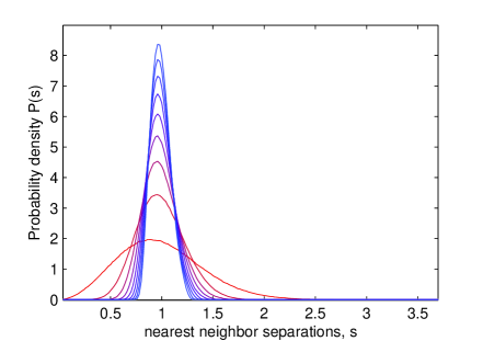
Figure 5: The histogram of the nearest neighbor separations $s_{n}=\frac{\gamma_{n+1}-\gamma_{n}}{2\pi}\ln\left(\frac{\gamma_{n}}{2\pi}\right)$ for 100,000 roots of the Riemann’s zeta function (found at A. Odlyzko’s website, $\mathop{\rm http://www.dtc.umn.edu/~{}odlyzko/zeta\mathop{\_}tables}$) and the separating sequences obtained using $\alpha_{n}^{(j)}=1/2$. Since the the first sequence in which the nearest neighbor separation magnitude does not exceed 1 it shows that the irregularity of Riemann zeros is less than 7. If the solutions (18) are used, then the complexity degree of the resulting hierarchy is 2.

The results of numerical analysis of the spectral fluctuations of quantum chaotic systems show that the probability of having large fluctuations decreases with the increase of hierarchy index $j$ (Fig 5). Although at the $0$th (physical) level of the hierarchy the histograms of various spectral statistics show the characteristic universal features BGS ; ABS , the shape of the distributions at the higher levels may deviate from them. Numerical studies indicate that the distribution of various spectral characteristics at the regular level (especially for the hierarchies with high $r$) tends to have a Gaussian-like shape, which develops through the hierarchy into different physical distribution profiles. For example, for the nearest neighbor statistics, $s_{n}^{(j)}=\left(1+\delta_{n+1}^{(j)}-\delta_{n}^{(j)}\right)$, it develops into Wignerian-like distribution, or, for $\delta_{n}^{(j)}$ or $\xi_{n}^{(j)}=\left(\delta_{n+1}^{(j)}+\delta_{n}^{(j)}\right)/2$ it develops into a Gaussian distribution with a larger variance, etc. A typical illustration of the appearance of the universal probability distribution profiles at the most disordered, $0$th, level of the hierarchy out of the distributions of the the regular, $r$th, level is shown on Fig. 5. Clearly, the support of the probability distribution functions becomes progressively wider with the approach to the physical level of the hierarchy. At the regular level, the range of the probability distribution function is defined by the condition $|\delta_{n}^{(j)}|<1$.

III Complexity of quantum graph spectra

In Opus ; Prima ; Sutra ; Stanza ; Anima ; Fabula ; Saga it was shown that this approach can be applied to the case of the quantum graphs – simple quasi one dimensional, scaling, classically stochastic models (Fig. 6), that are often used to model deterministic chaotic behavior in low dimensional dynamical systems QGT ; Gaspard .

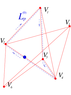
Figure 6: A 6 vertex quantum graph. Dashed line represents a periodic trajectory $p$ with the length $L^{(0)}_{p}$.

In Anima ; Saga ; Fabula it was shown that there exist quantum graphs with different degrees of spectral irregularity defined in the sense of the bootstrapping hierarchy. For the simplest case of the regular quantum graphs Opus ; Prima ; Sutra ; Stanza ; Wilmington , the spectrum obtained from (12) is given by

$$k_{n}^{(0)}=\frac{\pi n}{L_{0}}+\mathop{\rm Im}\sum\limits_{p}C_{p}^{(0)}e^{iL_{p}^{(0)}\frac{\pi n}{L_{0}}},$$ (19)

where the coefficients $C_{p}^{(0)}$ emerge from the parameters of the Gutzwiller’s series QGT ; Nova after the integration (12), $L_{0}$ is the total length of the graph bonds, and $L_{p}^{(0)}$s are the lengths of the periodic orbits $p$ on the graph.

The expansion (19) suggests a simple physical interpretation. As mentioned above, a quantum graph is regular, if its spectrum is sufficiently close to the periodic sequence

$$k_{n}^{(r)}=\frac{\pi n}{L_{0}}.$$ (20)

Incidentally, (20) defines the “integrable” spectrum of a point particle in a $1D$ box of the same overall size $L_{0}$. According to (19), the required corrections to (20) are given by the semiclassical amplitudes $e^{iS_{p}^{(r)}}$, where $S_{p}^{(r)}=L_{p}^{(0)}k_{n}^{(r)}$ are the values of the action functionals evaluated for all the available periodic motions in the system with the “integrable” momentum (20). So the $n$th level quantum wave that is geometrically consistent with the graph’s size, as it would be in the case infinite square well, now also circles simultaneously along all the possible periodic paths on the graph with the momentum (20). The resulting periodic orbit fluctuation amplitudes, combined with the right weights, produce the actual momentum eigenvalues for the nonintegrable system. Hence the exact “nonintegrable” values of $k_{n}^{(0)}$ also appear as the result of a complex interference effect similar to (3).

This represents a generalization of the EBK quantization formula for the case of quantum graphs, that allows to build the individual eigenvalues $k_{n}$ constructively, via the explicit functional dependence on the index $n$. The effect of classical nonintegrability appears in (19) as a “perturbation” to the integrable background pattern, if $k_{n}-\frac{\pi n}{L_{0}}<\frac{\pi}{L_{0}}$. In this aspect, the situation is reminiscent of the effect of persistence of the integrability structures in the phase space under small nonintegrable perturbations described by the KAM theory Arnold .

For the irregular graphs with several level spectral hierarchy, the relationship (19) is repeated for each transition between the hierarchy levels,

$$k_{n}^{(j)}=k_{n}^{(j+1)}+\eta^{(j+1)}+\mathop{\rm Im}\sum\limits_{p}C_{p}^{(j)}e^{iL_{p}^{(j)}k_{n}^{(j+1)}},$$ (21)

where $\eta^{(j+1)}$ is a bounded function of the fluctuations on the $j+1$ level, $\eta^{(j+1)}=\eta^{(j+1)}\left(\delta^{(j+1)}\right)$ Gratia ; Tantra ; Magna . Also in general, the harmonic expansion (21) is different from the periodic orbit expansion of (19), $C_{p}^{(j)}\neq C_{p}^{(0)}$ and $L_{p}^{(j)}\neq L_{p}^{(j)}$ Gratia ; Tantra ; Magna . Hence the $j$th level oscillations transmit the discrete momentum values from the $(j+1)$th to the $j$th level of the hierarchy. As a result, the “integrable spectrum” $k_{n}^{(r)}$ that explicitly carries the quantum number $n$ is adjusted $r$ times according to the set of equations (21) until it is transmitted from the regular to the $0$th level of the hierarchy. In Anima ; Saga ; Fabula it was sown that every graph is characterized by a finite irregularity degree.

It is important that a quantum graph of given topology can have different degrees of spectral irregularity depending on the bond length and other graph parameters Anima ; Saga ; Fabula . Since the geometric complexity of the periodic orbit set is defined by the topology of the graph, it means that spectral irregularity, as a complexity measure, is not a trivial reflection of the phase space complexity of the underlying classical system, and provides a separate characterization of the complexity of quantum spectra.

The expansions (19) and (21) can be used to describe analytically the development of the universal probability distributions Gratia ; Tantra ; Magna , illustrated on Fig. 5.

IV Discussion

The task of quantifying the complexity of the map between the natural numbers and a given sequence $x_{n}=x(n)$ is very general. This problem was recently considered in Arnold1 ; Arnold2 for the case of finite sequences over finite alphabets, which revealed a remarkably complex organizational structure of these mathematical objects. The complexity organization scheme developed in Arnold1 ; Arnold2 is generated by the linear difference operator

$$\Delta x(n)=x(n)-x(n+1)=x^{\prime}(n),$$ (22)

that maps one sequence into another. The motivation for using the operator $\Delta$ is that in certain simple cases it restricts the complexity of the symbolic sequences, i.e. it produces more ordered sequences out of less ordered ones. For example, the constant sequences $x_{n}\equiv x_{n}^{(0)}=\mathop{\rm const}$, are mapped into $x_{n}^{\prime}=\Delta x_{n}^{(0)}=0$, which is the “simplest” constant sequence. If $x_{n}$ is linear, $x_{n}=x_{n}^{(1)}=an+b$, then its image $x^{\prime}=\Delta x_{n}^{(1)}=x_{n}^{(0)}$ is a constant sequence, which is simpler than linear, so that $\Delta^{2}x^{(1)}=0$, and so on. In general, the functions for which $\Delta^{l}x=0$ for some $l$ are the polynomials of degree $m<l$, $x=p^{(m)}\in P_{l}$. Intuitively, the higher is the degree of the polynomial, the more complex is the mapping $x_{n}=x(n)$.

For the case of finite sequences, one necessarily runs not only into the polynomials, but also into more complex “exponential” functions. By definition, the function for which $\Delta^{l}x(n)=x(n)$ is an exponential polynomial $e^{(q)}\in E_{l}$ of the order $q$ that divides $l$. In Arnold1 ; Arnold2 it was shown that any function $f$ can be characterized by a polynomial degree $\deg(f)=\deg\left(p^{(m)}\right)=m$ and an exponential order $\mathop{\rm ord}(f)=\mathop{\rm ord}\left(e^{(q)}\right)=q$, which allows to formalize the organization of complexity of the sequences.

By definition Arnold1 ; Arnold2 , a function $x_{n}$ is more complex than $x_{n}^{\prime}$ if $\mathop{\rm ord}(x_{n})>\mathop{\rm ord}\left(x_{n}^{\prime}\right)$. If two sequences have the same order, $\mathop{\rm ord}\left(x^{\prime}_{n}\right)=\mathop{\rm ord}\left(x^{\prime}_{n}\right)$ then $x_{n}$ is more complex than $x^{\prime}_{n}$ if $\deg(x_{n})>\deg\left(x^{\prime}_{n}\right)$. This definition of the complexity scales is similar to the organization of the growth rates of the exponential polynomials as described e.g. in Levin . Empirical (e.g. numerical) studies of simple examples, e.g. of the binary sequences, show that it captures the intuitive idea that, e.g., $010101010101$ is simpler than $010001101111$, and helps to establish a number of beautiful relationships and a surprisingly rich complexity structure.

It is clear however, that the case of finite discrete sequences over finite alphabets is simpler than the case of the infinite sequences with real valued elements, as in the case of the spectral sequences. Although in some cases it is possible to study the complexity of discretized sequences Muchnik , for spectral sequences it is not clear a priori which discretization scheme should be used.

Using the bootstrapping hierarchy approach leads to a natural scale of complexity for the spectral sequences. The bootstrapping transformations suggested by the use of the Gutzwiller’s trace formula, also produce more ordered sequences out of less ordered ones, and generate a finite complexity degree for a number of systems, such as spectral sequences of quantum graphs or the nontrivial zeroes of the Riemann’s zeta function. This degree is analogous to the polynomial degree of the finite sequences as defined in Arnold1 ; Arnold2 .

However, an important feature of the finite sequence complexity structures established in Arnold1 ; Arnold2 via (22) is that they do not generalize in any trivial way when the length of a sequence is increased. On the one hand, in many applications, a given $N$-letter long sequence over an $M$-letter alphabet may appear as an approximation to a longer (e.g. infinite) $N_{1}$-letter long sequence, $N_{1}>N$, defined over a larger $M_{1}$-letter alphabet, $M_{1}>M$, and the task is to characterize the complexity of the entire sequence. Hence it is natural to use complexity measures that are stable with respect to such completions of shorter sequences by the longer ones. In the context of studying spectral sequences, complexity index defined for a sufficiently long list of elements should stabilize with the increase of sequence’s length, so that the spectrum as a whole is characterized by a single coherent complexity degree, that can be deduced from sufficiently long finite approximations.

In view of this, it is particularly significant that the degree produced by the bootstrapping method proposed above allows a stable characterization of the complexity of the whole spectral sequence. Numerical analysis of Riemann’s zeroes and of the spectra of quantum graphs of different topologies shows that the regularity degree obtained on the basis of a few hundred levels remains the same when a much larger ($10^{5}-10^{6}$) set of levels is considered.

It is also physically relevant that the expansion (3) is typically derived with a semiclassical accuracy, so the locations of the peaks generated by the sum (3) corresponds to the actual $E_{n}$ values only approximately. Moreover, even in cases when Gutzwiller’s formula is exact, as in the case of the quantum graphs QGT ; Nova and a few other systems Berry3 ; Gutzw ; Selberg ; Melrose the sum (3) cannot in general be computed exactly, because only a finite number of the periodic orbits may be known and their characteristics (e.g. the factor coefficients $B_{p}$ and the actions $S_{p}$) are described with a finite accuracy. Hence the harmonic expansions on each level of the hierarchy provide only a “fuzzy” description of the spectrum. It is therefore important that the regularity degree obtained via the bootstrapping method is also stable with respect to the using finite approximations to Gutzwiller’s sum, so the semiclassical description gives a correct estimate of the exact hierarchy index of complexity of quantum spectra.

The work was supported in part by the Sloan and Swartz Foundations.

References

- (1) V. I. Arnol’d, Mathematical Methods of Classical Mechanics, Springer (1989).
- (2) M. Gutzwiller, Chaos in Classical and Quantum Mechanics (Springer, New York, 1990).
- (3) P. Cvitanović, et al, Classical and Quantum Chaos, Niels Bohr Institute, Copenhagen, (1999).
- (4) A. Selberg, Journal of the Indian Mathematical Society 20, pp. 47-87 (1956).
- (5) T. Kottos and U. Smilansky, Ann. Phys. 274, 76 (1999).
- (6) F. Barra and P. Gaspard, Phys. Rev. E 63 066215 (2001).
- (7) Y. Dabaghian, R. V. Jensen, and R. Blümel, Phys. Rev. E 63, 066201 (2001).
- (8) R. Blümel, P. M. Koch and L. Sirko, Foundations of Physics, 31 (2) p. 269 (2004).
- (9) M.V. Berry and J.P. Keating, SIAM Review, 41, No. 2, pp. 236-266 (1999).
- (10) M.V. Berry and J.P. Keating, Proceedings of the Royal Society of London A, Vol. 437, pp. 151-173.
- (11) M.V. Berry, Proceedings of the Royal Society of London A Vol. 413 pp. 183-198, (1987).
- (12) E. Bogomolny, Chaos, Vol. 2, Issue 1, pp. 5, (1992).
- (13) H. Bohr, Almost Periodic Functions. New York: Chelsea (1947).
- (14) A. S. Besicovitch, Almost Periodic Functions. New York Dover (1954).
- (15) C. Corduneanu, Almost Periodic Functions. New York, Wiley Interscience (1961).
- (16) H. P. Baltes and E. R. Hilf, Spectra of Finite Systems, BI Wissenschaftsverlag, Mannheim (1976).
- (17) Y. Dabaghian and R. Blümel Phys. Rev. E 68, 055201(R) (2003).
- (18) Y. Dabaghian and R. Blümel JETP Letters 77, n 9, p. 530 (2003).
- (19) Y. Dabaghian and R. Blümel, Phys. Rev. E 70, 046206 (2004).
- (20) Y. Dabaghian, R. V. Jensen and R. Blümel, JETP Letters 74(4), 235-239 (2001).
- (21) R. Blümel Y. Dabaghian, R. V. Jensen, Phys. Rev. Lett. 88, 044101 (2002).
- (22) R. Blümel Y. Dabaghian, R. V. Jensen, Phys. Rev. E (2001).
- (23) Y. Dabaghian, R. V. Jensen and R. Blümel, JETP Vol.121, N6 (2002).
- (24) Y. Dabaghian, R. V. Jensen, and R. Blümel, Proceedings of Fourth International Conference on Dynamical Systems and Differential Equations, Wilmington, NC, pp. 206-212 (2002).
- (25) Y. Dabaghian, JETP Letters, Vol. 83(12), pp. 587-592 (2006).
- (26) Y. Dabaghian, Phys. Rev. E 75, 056214 (2007).
- (27) Y. Dabaghian, Theoretical and Mathematical Physics, to appear (2007).
- (28) M. Li and P. Vitanyi, Math. Systems Theory 27, 365-376 (1994).
- (29) An. Muchnik, A. Semenov and M. Ushakov, Theoretical Comp. Sci. 304 pp. 1 – 33 (2003).
- (30) V. I. Arnol’d, Functional Analysis and Applications, Vol. 1(1), pp. 1–18 (2006).
- (31) V. I. Arnol’d, Russ. Math. Survey, Vol. 58(4), pp. 637-664 (2003).
- (32) O. Bohigas, M.-J. Giannoni, C. Schmidt, Phys. Rev. Lett. 52, 1 (1984).
- (33) R. Aurich, J. Bolte, and F. Steiner, Phys. Rev. Lett. 73, 1356–1359 (1994).
- (34) B. Ya. Levin, Distribution of Zeroes of Entire Functions, Am. Math. Society, Providence, (1980).
- (35) K. G. Anderson and R. B. Melrose, Inv. Math. 41, 197 (1977).