Resumming Cosmological Perturbations via the Lagrangian
Picture:
One-loop Results in Real Space and in Redshift Space
Abstract
We develop a new approach to study the nonlinear evolution in the large-scale structure of the Universe both in real space and in redshift space, extending the standard perturbation theory of gravitational instability. Infinite series of terms in standard Eulerian perturbation theory are resummed as a result of our starting from a Lagrangian description of perturbations. Delicate nonlinear effects on scales of the baryon acoustic oscillations are more accurately described by our method than the standard one. Our approach differs from other resummation techniques recently proposed, such as the renormalized perturbation theory, etc., in that we use simple techniques and thus resulting equations are undemanding to evaluate, and in that our approach is capable of quantifying the nonlinear effects in redshift space. The power spectrum and correlation function of our approach are in good agreement with numerical simulations in literature on scales of baryon acoustic oscillations. Especially, nonlinear effects on the baryon acoustic peak of the correlation function are accurately described both in real space and in redshift space. Our approach provides a unique opportunity to analytically investigate the nonlinear effects on baryon acoustic scales in observable redshift space, which is requisite in constraining the nature of dark energy, the curvature of the Universe, etc., by redshift surveys.
pacs:
98.80.-k, 95.35.+d, 95.36.+x, 02.30.MvI Introduction
Recent progress in cosmology is largely stimulated by precise measurements of the Universe. The redshift survey of galaxies is one of the most important methods in distinguishing cosmological models. The baryon acoustic oscillations (BAOs) in the early universe BAOtheory , which were first detected in the cosmic microwave background (CMB) anisotropy power spectrum CMBobs , were also detected in the large-scale structure probed by redshift surveys BAOLSS . The expansion history and curvature of the Universe can be geometrically measured by galaxy clustering in redshift space AP79 ; GeomTest , and the BAO signature in the large-scale structure yields a standard ruler BAOSR for this purpose. Therefore, accurately measuring the BAO scales in a statistical quantity such as the power spectrum or correlation function of galaxies, one can constrain the structure of the Universe, such as the nature of dark energy BAODE .
To utilize the BAOs as a standard ruler in the Universe, a theoretically precise description of the BAOs is of the utmost importance. The physics of the BAOs at sufficiently large redshift is well described by linear theory. Only the amplitude of the spatial pattern of clustering is increased, and the characteristic scale of the BAOs is unaltered in this regime. However, the nonlinear dynamics play an important role in a redshift range where we can measure the large-scale structure. Even though the BAO scales are large, the nonlinearity deforms the BAO pattern in the power spectrum and correlation function SE05 ; Spr05 ; BAONL ; BAONLRD ; ang07 ; ESW07 . Nonlinear deformations of the power spectrum are described by the standard perturbation theory (SPT) jus81 ; vish83 ; Fry84 ; Goroff86 ; MSS ; JB94 ; BCGS02 of higher orders as long as the density fluctuations on BAO scales are still in the linear regime at sufficiently large redshift MWP99 ; JK06 . The last condition is not necessarily satisfied by realistic surveys. Moreover, when the cold dark matter (CDM) is present, the higher-order SPT does not give any sensible prediction for the correlation function because unphysical behavior in small wavelength limit prevents Fourier transform from converging.
Recently, several other approaches beyond the framework of SPT have been proposed Sco01 ; NewPT ; CS06a ; CS06b ; Val07 ; CS07 ; RGPT ; TH07 . Among others, Scoccimarro’s reformulation of fluid equations using the propagator, the vertex, and a source Sco01 provides a way to use standard tools of field theory, yielding the renormalized perturbation theory (RPT) CS06a ; CS06b ; CS07 , the large- expansions Val07 , the renormalization group approach RGPT , and the closure theory TH07 in the context of gravitational instability theory. In these newly developed approaches, the standard perturbative expansion is reorganized and partially resummed in various ways. It is still difficult to exactly calculate the power spectrum by these approaches, and different levels of approximations and ansatz are employed. The predictions of the power spectrum calculated by the 2-loop RPT and renormalization group method are shown to agree with measurements of the -body simulations on BAO scales even at low redshift where the 1-loop SPT breaks down CS07 ; RGPT . It is still nontrivial why these approaches work well despite their approximate treatments and use of ansatz.
So far the predictions of the above nonlinear theories, such as SPT, RPT, and their variants, have been confined in real space. Since the large-scale structure is actually measured in redshift space, it is mandatory to make predictions in redshift space for applying the nonlinear theories to realworld observations. The redshift-space distortion effects in the linear regime are analytically given by first-order SPT (i.e., linear theory) Kaiser87 ; Ham92 ; GeomTest . However, investigations of nonlinear redshift-space distortions by higher-order SPT are quite limited in literature HMV98 ; SCF99 , apart from numerical simulations and nonlinear modelings MWP99 ; BAONLRD ; ang07 ; Sco04 ; SE05 ; ESW07 .
In this paper, we consider resummations of the perturbative expansion by a different approach from RPT and its variants. Instead of relying on Scoccimarro’s reformulation, we start from a Lagrangian picture of density perturbations. Why do we have to add yet another approach even though there are already enough? There are a number of reasons. First, our approach is simpler than other resummation methods. While it is straightforward to calculate the power spectrum in our approach, other resummation techniques are so complicated that approximate treatments and/or ansatz are necessary in deriving the final power spectrum. Second, as a result of that, our analytic expression of the resulting power spectrum is no more complicated than the SPT expression, and numerical evaluations are fast performed. Third, and most importantly, our approach is capable of evaluating the nonlinear power spectrum in redshift space, which is beyond the scope of other resummation methods in literature. Fourth, unlike in SPT, the power spectrum in our approach can be Fourier transformed to predict the nonlinear effects in the correlation function.
An important ingredient of our approach is the perturbation theory in Lagrangian space, which is known as the Lagrangian perturbation theory (LPT) LPT . The first-order LPT corresponds to the classic Zel’dovich approximation Zel70 . Since the observable power spectrum is given in Eulerian space, predicting the power spectrum by LPT is not a trivial task. We define a method of calculating the power spectrum from the LPT, partially expanding the Lagrangian variables in Eulerian space. The resulting expression contains an infinite series of SPT terms; that is, the SPT terms are automatically resummed in our formulation. The underlying motivation of this formulation is shared with RPT. Readers are recommended to go through an excellent introduction in Ref. CS06a using the Zel’dovich approximation, which equally applies to our formulation since our formalism and RPT become equivalent in a case of Zel’dovich approximation.
The rest of this paper is organized as follows. In Sec. II, our basic formalism is described. A brief review of LPT is also included. In Sec. III, analytic results of the power spectrum and correlation function in real space are presented and compared with simulation results in the literature. The corresponding results in redshift space are derived in Sec. IV. The conclusions are given in Sec. V.
II Resumming Perturbations via the Lagrangian Picture
II.1 The power spectrum from the Lagrangian variable
In a Lagrangian picture, a fundamental variable to represent perturbations is a displacement field , which maps a fluid element from initial Lagrangian coordinates to the Eulerian coordinates at a time :
| (1) |
We will drop the argument in the following for notational simplicity, and readers should keep in mind that the dynamical variables always depend on time.
Assuming the initial density field is sufficiently uniform, the Eulerian density field satisfies the continuity relation, , where is the mean density in comoving coordinates. This relation is equivalent to the following equation:
| (2) |
where is the density contrast. The power spectrum is defined by a relation
| (3) |
where
| (4) |
is the Fourier transform of the density contrast. The power spectrum in real space depends only on the magnitude of the wave vector, . In redshift space, however, a directional dependence emerges. Using Eqs. (2)–(4), the power spectrum can be expressed by a displacement field as TaylorPS
| (5) |
where . Because of the homogeneity, the ensemble average in the integrand of the right-hand side (RHS) only depends on the separation . The expression of Eq. (5) is a general relation between the power spectrum and displacement fields.
We use the cumulant expansion theorem Ma85
| (6) |
in Eq. (5), where denotes a cumulant of a random variable BCGS02 . In the resulting equation, we have a following quantity:
| (9) |
where the binomial theorem is applied. In this equation, only cases are survived, because for parity symmetry. Accordingly, we obtain a general expression,
| (10) |
where summation over repeated indices is assumed as usual, and
| (11) | |||
| (14) | |||
| (15) |
are defined. In the RHS of Eq. (15), all the indices are symmetrized over.
The quantity of Eq. (11) is given by a cumulant of a displacement vector at a single position. The quantity of Eq. (15) is given by cumulants among two displacement vectors which are separated by a Lagrangian distance . Correlations among components of separated displacement vectors are expected to be small when the separations are large. When we are interested in clustering on large scales, the magnitude of wave vector is small, and large separations of in Eq. (5) efficiently contribute to the integral. Therefore, we expect the cumulants of are smaller than the cumulants of on large scales.
With the above consideration, we propose to expand only the terms in Eq. (10) as small quantities and keep the terms in the exponent. If the terms are expanded as well, this equation turns out to give equivalent results of SPT, which is formulated in Eulerian space, as shown below. Therefore, the exponential prefactor contains infinitely higher-order perturbations in terms of SPT. Thus our method provides a way to resum the infinite series of perturbations in the SPT. This point is our first key technique of this paper. The second technique is to evaluate the cumulants of the displacement field by the LPT, which is addressed in the following. Before that, it is convenient to represent the cumulants of the displacement field in Fourier space.
II.2 Polyspectra of the displacement field
To evaluate Eq. (10), it is useful to define the polyspectra of the displacement field by
| (16) |
where
| (17) |
is the Fourier transform of the displacement field. The relation is always satisfied because of the translational invariance. For , we employ a notation, , for simplicity. The factors in the RHS of Eq. (16) are there to ensure that the polyspectra are real numbers. In fact, one easily finds the complex conjugate satisfies
| (18) |
which is an equivalent condition that the polyspectra are real numbers, . It is also important to note the polyspectra of the displacement field satisfy a parity relation,
| (19) |
II.3 The Lagrangian perturbation theory
For a Newtonian pressureless self-gravitating fluid embedded in an expanding universe, the displacement field is governed by the equation of motion,
| (25) |
where is the time-dependent Hubble parameter, and is a derivative with respect to the Eulerian coordinate, . The gravitational potential is determined by the Poisson equation,
| (26) |
where the density contrast is related to the displacement field by Eq. (2) or, equivalently,
| (27) |
We use the LPT LPT to evaluate the polyspectra of the displacement field. In LPT, the displacement field is expanded by a perturbative series:
| (28) |
where has the order of , which is considered a small quantity (properly speaking, dimensionless quantity is considered to be small). It is quite common in the LPT that the velocity field is assumed to be irrotational,
| (29) |
This condition is compatible with the dynamical Eq. (25) and restricts one to considering a subclass of general solutions. The main motivation of this restriction is that the vortical motions linearly decay in Eulerian perturbation theory BCGS02 and thus are negligible in the quasilinear regime. We assume this condition throughout this paper. The longitudinal part of Eq. (25) is an independent equation to be solved perturbatively in LPT; the same is true for Eqs. (26), (27), and (29). Each perturbative term of the displacement field in Fourier space is generally represented as
| (30) |
where is the linear density contrast at the present time , is a linear growth rate normalized by . The imaginary unit is there to ensure that the perturbative kernels are real vectors. This is straightforward to show by considering the parity transformation of both sides of Eq. (30). The perturbative kernels do not depend on time in an Einstein–de Sitter model. In general cosmology, they weakly depend on time and cosmological parameters BCHJ95 . It is still a good approximation that the perturbative kernels in arbitrary cosmology are replaced by those in the Einstein–de Sitter model BCGS02 . We adopt this approximation throughout this paper for simplicity, although including such dependence is straightforward. The perturbative kernels in LPT up to third order are given by Cat95
| (31) | |||
| (32) | |||
| (33) |
where for , and a vector represents a transverse part whose expression is not needed in the following application. It is useful to symmetrize the kernel in terms of their arguments:
| (34) |
II.4 One-loop approximation to the resummed power spectrum
The polyspectra of the displacement field in LPT can be evaluated in almost the same way as in the case of density fields in Eulerian perturbation theory. Substituting Eqs. (17), (28), and (30) into Eq. (16), the perturbative expansion of the polyspectra is calculated. We assume the initial density field is a random Gaussian field, in which case the cumulants of the linear density field are completely expressible by a linear power spectrum, . Up to second order in , we obtain
| (35) | |||
| (36) |
where we define quantities , by
| (37) | |||
| (38) |
which are explicitly given by using LPT kernels as
| (39) | |||
| (40) | |||
| (41) |
and
| (42) |
The polyspectra of order four or higher do not contribute up to second order in . In random Gaussian fields, it can generally be shown that -polyspectrum has the order in , for the connectedness of the cumulants. In SPT, diagrammatic techniques prove to be quite useful Goroff86 ; SF96 . Similarly, we find diagrammatic representations of the above quantities of Eqs. (39)–(42), which are given in Fig. 1.
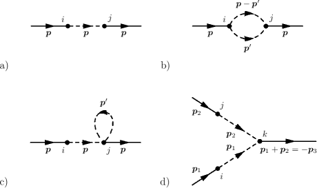
At this point, Eq. (10) is expanded by LPT by using Eqs. (20), (24), and (39)–(42). As promised, only quantities are expanded from the exponent in Eq. (10) and keep in the exponent. The result is
| (43) |
Except for the linear-theory contribution, , all the polyspectra in the above terms are accompanied by integrations over wave vectors. Accordingly, these terms correspond to the 1-loop diagrams in Fig. 2.

The bubble diagram (a) of Fig. 2 corresponds to the exponent of the first factor. The tree diagram (b) corresponds to the linear contribution , and loop diagrams (c)–(e) correspond to , , and , respectively. The loop diagrams (f)–(h) correspond to integrals of , , and , respectively. The last loop diagram i) corresponds to the last integral in Eq. (43). The expansion of Eq. (43) is therefore a loop expansion, and all the 1-loop diagrams are exhausted in this equation. In the exponent of the prefactor, we could consider the higher-order terms such as integrals of , . These terms correspond to the 2-loop diagrams of Fig. 3.

Although those terms are second order in , their contributions to the total power spectrum are third order since they are multiplied by first- or higher-order terms in Eq. (43). Therefore, we do not include these 2-loop contributions and truncate all the multiloop contributions.
III Clustering in Real Space
III.1 The power spectrum
It is straightforward to calculate Eq. (43) using the expression of the polyspectra of the displacement field, Eqs. (39)–(42), and perturbation kernels, Eqs. (31)–(34). Contractions with spatial indices in Eq. (43) can be taken before evaluating the momentum integrations. The transverse part in the third-order kernel, Eq. (33), vanishes in course of calculation, because of the inner product with vector . As a result, the calculation is quite similar to that in SPT, where some of the angular integrations can be analytically done MSS . The result is
| (44) |
Comparing this result with that of 1-loop SPT MSS , one immediately notices the similarity of the equations. The only differences are the existence of the exponential prefactor and the number of the second term in the last square bracket, which is in SPT instead. Thus, Eq. (44) is equivalently represented as
| (45) |
where is a pure 1-loop contribution (without a linear contribution) to the power spectrum in SPT. It is obvious from this expression that expanding the exponential prefactor exactly reproduces the SPT result at the 1-loop level. The exponential prefactor contains information from an infinite series of higher-order perturbations in terms of SPT. In terms of diagrams of SPT Goroff86 , the exponential prefactor comes from the diagrams in which two points are connected by a single internal line with but vertices are dressed by loops. However, those diagrams are not completely resummed, and parts of the resulting terms are resummed. Therefore, the resummation of this paper corresponds to a partial vertex renormalization in terms of the SPT.
On the other hand, the resulting expression has a certain similarity with RPT CS06a ; CS06b , because of the exponential prefactor. In fact, a square root of this factor coincides with the nonlinear propagator in a large- limit of RPT. In its formulation, the nonlinear power spectrum is divided into two parts. The first part is linearly dependent on the initial power spectrum with a coefficient given by the square of the propagator. The second part corresponds to contributions from mode couplings among different scales. RPT uses loop expansions to evaluate the mode-coupling contributions. Our expression has a similar structure, although the methods are quite different. One possible reason for this similarity is that the RPT propagator in the Zel’dovich approximation exactly coincides with the square root of the exponential prefactor of Eq. (44) above. In the Zel’dovich approximation, only is present for cumulants of the displacement field. As a result, loop corrections come only from diagrams of type i) in Fig. 2 and its multiloop extensions (-loop diagrams with internal lines connected to the two external vertices), in which the vertex renormalization cannot appear. As a result, RPT and our approach turn out to be equivalent in the Zel’dovich approximation (see the introduction of Ref. CS06a ).
Having an exponential damping factor, the power spectrum in our approximations does not have power at large wave numbers. This behavior is not physical in the fully nonlinear regime, since the nonlinear evolution enhances the power spectrum on small scales. Our approximations only apply to the quasilinear regime on large scales. An advantage of this property is that the integration of the power spectrum is stable so that other statistical quantities may be obtained, such as the correlation function, on quasilinear scales.
On the other hand, our approximations for the power spectrum itself fail when the exponential damping factor is efficient. It is useful to have an estimate for the validity range of wave numbers in our approximations. Since the damping scale is given by
| (46) |
a possible criterion for the validity range is , where should be determined according to the required accuracy. We will see below that corresponds to the accuracy within a few percent, compared to the -body simulations. Throughout the rest of this paper, we consider as the validity range in our approximations.
In Fig. 4, the power spectra of our result, and those of linear theory and 1-loop SPT, are compared.
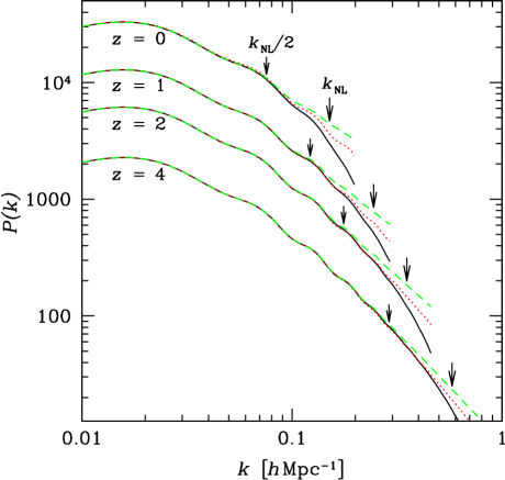
The linear power spectrum is calculated from the output of CMBFAST CMBFAST at . We adopt a cosmological model with parameters , , , , and . The damping scale and the claimed validity scale are indicated in the figure. It is clearly seen that our power spectra are expnentially damped on small scales . In this log-log plot, differences among the three approximations in our claimed validity range are hardly seen. Our approach is advantageous when a very accurate estimation on large scales is crucial. The determination of the BAO scale really requires such accuracy.
In Fig. 5, detailed features in nonlinear power spectra are shown on BAO scales.
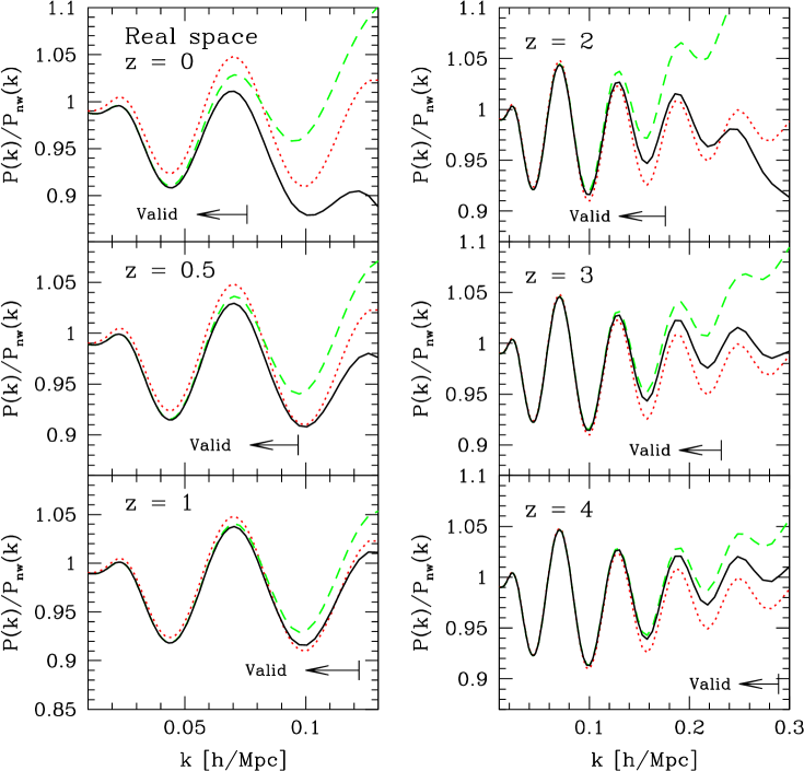
To enhance the baryon oscillations, each power spectrum is divided by a smoothed, no-wiggle linear power spectrum EH99 . The same cosmological parameters are assumed as in Fig. 4. The validity ranges are indicated in the figure. There are differences among three approximations in our validity ranges.
In Fig. 6, our result of the power spectrum in real space is compared with the -body simulations of Ref. SE05 using the same parameters as Seo and Eisenstein’s.
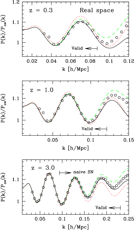
In this case, and other cosmological parameters are the same as above. The linear power spectrum is calculated from the output of CMBFAST at to match the input power spectrum of the simulations. Since the no-wiggle power spectrum matches to the power spectrum at , the baseline is slightly larger than unity, because of nongravitational effects in the transfer function. To reduce the effects of cosmic variance in -body simulations, we calculate the differences (in logarithmic scales) between the output power spectra and linearly evolved initial power spectra at , both measured in simulations. The resulting differences are added to the linear theory prediction in the figure. In this way, initial deviations of the power spectrum from the theoretical power spectrum are subtracted (similar presentations are seen in Ref. Spr05 ). The actual output power spectrum of simulations is noisier than that in the figure especially on larger scales. As described in Ref. SE05 , the Savitzky-Golay filtering is applied when the power spectrum in each -body sample is evaluated. The shot noise is not corrected for the -body samples, since the initial positions of particles are on regular grids, and the naïve shot noise , where is the number density of particles, does not apply at a large redshift in the simulation Seo07 . It is not obvious how to correct for the shot noise in such a situation. The samples with and are hardly affected by the shot noise because the signal amplitudes are large, but contributions from the naïve shot noise in the sample are over for . Therefore, the sample could be more or less affected by nontrivial shot noise in that range, although that is smaller than the naïve shot noise.
In all cases of the three redshifts , , , the ranges where our results and simulations agree are broader than those of 1-loop SPT. Overall, the 1-loop SPT overestimates the power spectrum on relatively small scales, while our result is always better on the same scales. For example, the height of the peak at of the sample is explained by our work, while the 1-loop SPT overestimates the height. In a range – of the sample, -body data are (accidentally) closer to the linear theory rather than the 1-loop SPT. This tendency is also explained by our work. In the sample, our result matches the -body result in the range , while linear theory and 1-loop SPT do not (under the condition that the nontrivial shot noise is negligible as noticed above). The simulations and our results agree within a few percent in our claimed validity range, .
III.2 The correlation function
The correlation function is given by a Fourier transform of the power spectrum. After angular integrations, they are related by
| (47) |
where is the spherical Bessel function of zeroth order.
In the 1-loop SPT, the power spectrum badly behaves on small scales to perform this integral. The 1-loop contribution to the power spectrum in SPT consists of two terms, . Each term asymptotically behaves as vish83 ; MSS
| (48) |
and the net power spectrum is much smaller in magnitude than each term. On mildly small scales, the residuals also behave as for a CDM-like power spectrum. Therefore, the power spectrum on small scales contributes to the integral in Eq. (47) even if the separation is large. In a small-scale limit, , the leading contributions of the two terms are exactly canceled out, and the net contribution behaves as vish83 ; MSS
| (49) |
For a CDM-like power spectrum, , and the integral in Eq. (49) diverges. As a result, one cannot evaluate the correlation function by the 1-loop SPT, because the integral of Eq. (47) does not converge. This divergence obviously reflects the fact that the 1-loop SPT is invalid on small scales. Since the correlation function is an observable quantity, this is an undesirable property in SPT. Such a problem does not occur in our expression of Eq. (44): the power spectrum is exponentially suppressed in the small-scale limit. This behavior is not physical on sufficiently small scales, since our expression is applicable only to the weakly nonlinear regime. However, small-scale behavior in the power spectrum should not be relevant to the correlation function on large scales, since dominant contributions of the power spectrum to the correlation function of Eq. (47) come from scales for a CDM-like power spectrum.
Since the exponential prefactor in Eq. (44) acts as a Gaussian damping function, the resulting correlation function has a form of convolution by a Gaussian smoothing function. This smoothing effect by nonlinearity is already known, which smears the BAO peak in the correlation function ESW07 . The physical origin of this nonlinear smearing is the random motion of mass elements, because the dominant contribution of this smearing factor comes from as obviously seen by Eqs. (10) and (11). It is worth noting that this nonlinear smearing effect is not captured by linear theory and higher-order SPT.
In Fig. 7, the nonlinear correlation function is plotted on BAO scales.
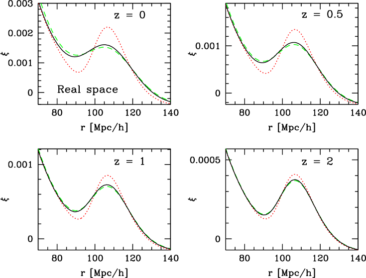
The same cosmological parameters as in Fig. 5 are adopted. Nonlinear smearing effects on the baryon acoustic peak are described by our theory. In Fig. 7, Gaussian-filtered linear theory is overplotted. The filtering length is given by the one that the exponential prefactor in Eq. (44) implies:
| (50) |
This simple model approximately explains the nonlinear smearing effects. In detail, this simple model overestimates the small-scale clustering and height of the trough, and underestimates the peak height.
In Fig. 8, our result of the correlation function in real space at is compared with the -body simulations of Refs. SE05 ; ESSS07 using the same parameters as used in these references.
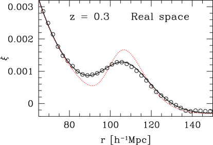
As in the case of the power spectrum, we compute differences (in linear scales) between the output correlation function and the linearly evolved initial correlation function at in the simulation, and the resulting differences are added to the linear-theory prediction in the figure. If we directly plot the measured correlation function, the amplitudes on – and – are slightly (about ) larger. This tendency is already seen even in the initial correlation function at , which can be identified to the finiteness effect of the simulations. Therefore, we only measure the nonlinear deviations from the linear theory in the simulation.
The agreement between the simulation and our result is quite good. There is not any fitting parameter at all. In the corresponding power spectrum, the plot in Fig. 6, the difference between our result and that of 1-loop SPT may seem to be small. In the correlation function, however, the difference is really big, since the 1-loop SPT cannot predict the correlation function, while our result explains the nonlinear effects on BAO scales very precisely.
IV Clustering in Redshift Space
IV.1 Mapping from real space to redshift space
Our approach above can be extensible to the calculation in redshift space. In redshift surveys, the position of each galaxy is measured by the redshift. In a completely homogeneous universe, the comoving distance–redshift relation is given by a standard formula for the Friedmann-Lemaître universe:
| (51) |
where is the time-dependent Hubble parameter. In reality, however, the Universe is locally inhomogeneous, and the comoving distance to a galaxy of redshift is not exactly given by Eq. (51). For the galaxy redshifts, the leading source of the deviation is the Doppler shift caused by the peculiar velocities of the galaxy. The observed redshift with the effect of the peculiar velocity can be calculated by solving the geodesic equation. The comoving distance in redshift space is defined by , where, in the RHS, the redshift-distance relation of Eq. (51) is adopted even though we live in an inhomogeneous universe. When the peculiar velocities are nonrelativistic, the comoving distance in real space, , and that in redshift space is related by TM2000 , where is a line-of-sight component of the peculiar velocity . Throughout this paper, we work in “distant-observer” or “plane-parallel” approximation, where the line-of-sight direction is fixed in space and denoted by . We ignore the contribution from the peculiar velocity of the observer, which does not contribute to the following calculation of the power spectrum. When the curvature scale of the Universe is much larger than clustering scales we are interested in, we can safely use local Cartesian coordinates in the volume of galaxy surveys. Thus the relation between the position in real space and that in redshift space is given by
| (52) |
where . Therefore, using Eq. (1), the displacement field in redshift space is given by
| (53) |
A similar equation has been applied to the analysis of the Zel’dovich approximation TH96 .
In the time-independent approximation to the perturbative kernels, , and therefore, the time derivative of the displacement field is simply
| (54) |
where is the logarithmic derivative of the linear growth rate. Thus, the displacement field of each perturbation order in redshift space is given by
| (55) |
which is just a linear mapping of the displacement vector of each order. This linear transformation is characterized by a redshift-space distortion tensor for th order perturbations, defined by
| (56) |
with which Eq. (55) reduces to , or in a vector notation, . Therefore, the perturbative kernels in redshift space are given simply by
| (57) |
Thus, our calculation in real space can be simply generalized to that in redshift space by using the redshift-space perturbative kernels in Eqs. (39)–(42), while the form of Eq. (43) is unchanged in redshift space, provided that the cumulants of the displacement field are evaluated in redshift space. The mappings of the order-by-order cumulants are quite simple:
| (58) | |||
| (59) |
IV.2 The power spectrum in redshift space
The calculation of Eq. (43) in redshift space is more complicated than in real space, since the anisotropy is introduced by the redshift-space distortion tensors. Accordingly, the momentum integrations should be evaluated before taking inner products with the vector . In redshift space, however, the cumulants and in Eq. (43) should be replaced by redshift-space counterparts, and of Eqs. (58) and (59). Since the redshift distortion tensors are anisotropic, the integrands do not reduce to scalar functions. Therefore we need to explicitly evaluate integrals of tensors. The results are given in Appendix A, Eqs. (85)–(87) and (89)–(91). Using those equations, it is straightforward to obtain an expression of the power spectrum in redshift space. There are many terms in the result, which are arranged as
| (60) |
where is the direction cosine of the wave vector with respect to the line of sight,
| (61) |
and
| (62) | |||
| (63) | |||
| (64) | |||
| (65) | |||
| (66) | |||
| (67) | |||
| (68) | |||
| (69) | |||
| (70) |
and all the other which are not listed above are zero. The functions and are given by Eqs. (77)–(84) in Appendix A.
As in the case of real space, the SPT result should be reproduced by expanding the exponential prefactor in Eq. (60). A formal expression for the 1-loop power spectrum in redshift space HMV98 contains 3-dimensional integrations. Further reduction of the expression is possible and necessary to compare with our result. In Appendix B, we derive a reduced expression for the power spectrum of 1-loop SPT in redshift space, which itself is a new result. Finally, the following relation, which is similar to Eq. (45), is confirmed:
| (71) |
where is the 1-loop contribution to the redshift-space power spectrum in SPT given in Appendix B. Therefore, when the exponential prefactor is expanded, Eq. (60) reduces to the result of SPT.
The linear term in Eq. (60) corresponds to the Kaiser formula Kaiser87 of the linear perturbation theory. The appearance of the exponential suppression prefactor is characteristic in our formalism. This factor reflects the nonlinear smearing effect of the velocity field along the lines of sight Jackson72 , such as the fingers-of-God effect by large-scale random motions. The linear theory and higher-order SPT do not have such a suppression factor along the lines of sight.
This form of the suppression factor exactly matches a phenomenological model of the redshift-space power spectrum on large scales ESW07 , which is given by (after correcting obvious typos)
| (72) |
where and are wave vector components across and along the line of sight, and and are modeled by
| (73) |
The length parameter characterizes the scale of radial displacements. When all the 1-loop contributions of our Eq. (60) are omitted, the model of Eq. (72) is “derived” if we identify , where is a linear-theory value of at . In Ref. ESW07 , the parameter is measured from the -body simulation of Eisenstein, Seo, and White, and a value is obtained for separations in their cosmology (we convert their quoted value according to different conventions of the growth factor). Using the same set of cosmological parameters as theirs, we find . The corresponding prediction from our formalism is , which is very close to their measured value.
There is another simple model of the nonlinear power spectrum in redshift space Sco04 , which is given by
| (74) |
where is the same as our of Eq. (61), and , , are (cross) power spectra of density and velocity fields, calculated from nonlinear 1-loop SPT. Even though the density and velocity (cross) correlations are taken into account, this model is no longer a result of exact 1-loop perturbation theory (see Appendix B). This simple model explains -body data to some extent but predicts a slightly larger power spectrum than -body data on small scales Sco04 . This model has a similar structure to our result but lacks many terms.
The spherical average of Eq. (60) is calculated by using the following integral:
| (75) |
where is the lower incomplete gamma function, and is the error function normalized by .
In Fig. 9, the spherically averaged nonlinear power spectrum in redshift space is plotted on BAO scales.
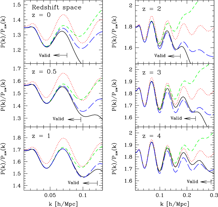
The same cosmological parameters as in Fig. 4 are adopted. Each power spectrum is normalized by a no-wiggle power spectrum EH99 in real space. According to the Kaiser effect, the amplitude is larger in higher redshifts. In the same plot, the simple model of Eq. (74) is overplotted. Both linear theory and 1-loop SPT are larger than our result and the simple model, since the former two do not have a suppression factor which corresponds to nonlinear smearing effects along the lines of sight in redshift space. The validity ranges are indicated in the figure, where is given by Eq. (46).
In Fig. 10, a comparison of the power spectrum in redshift space between our results and the -body simulations of Ref. SE05 is presented.
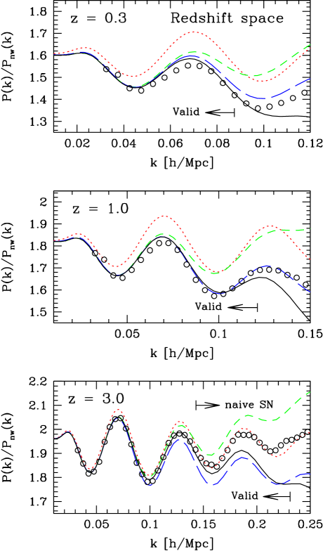
As in real space, our results are better than 1-loop SPT results. The 1-loop SPT overestimates the power spectrum much worse in redshift space. On smaller scales, the simple model of Eq. (74) and the linear theory seems to be good descriptions at a particular redshift. However, that is just a coincidence because they do not describe the simulations at different redshifts. The shot noise is not corrected for the -body simulation, and the -body sample of might be affected by the shot noise on small scales. The range where the naïve shot noise is over is indicated in the figure. Since the particle positions in redshift space are more randomly distributed than in real space, the true shot noise might be larger than that in real space. Overall, our results describe the -body results well at all redshifts.
IV.3 The correlation function in redshift space
The correlation function in redshift space is given by
| (76) |
When we consider the spherically averaged correlation function, the relation of Eq. (47) is applicable with the spherically averaged power spectrum.
In Fig. 11, the spherically averaged nonlinear correlation function in redshift space is plotted on BAO scales.
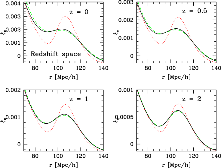
The same cosmological parameters as in Fig. 5 are adopted. Since the effect of the suppression factor is larger in redshift space, the nonlinear smearing effects on the baryon peak are larger than in real space (cf. Fig. 7). This is because the nonlinear redshift-space distortions additionally smear the clustering along the line of sight. As in Fig. 7, Gaussian-filtered linear theory is overplotted, which approximately explains the nonlinear smearing effects.
In Fig. 12, our result of the correlation function in redshift space at is compared with the -body simulations of Refs. SE05 ; ESSS07 using the same parameter as used in these references.
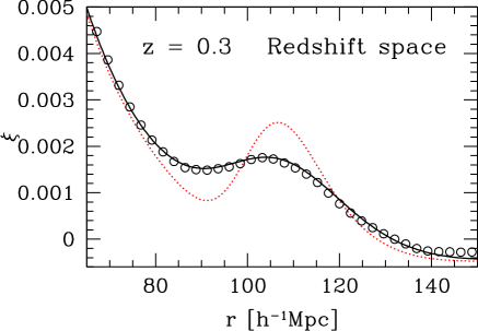
The agreement is quite good also in redshift space, and our result explains the nonlinear effects on BAO scales very precisely even in redshift space.
V Conclusions
In this paper, we have formulated a new resummation method of the cosmological perturbation theory, starting from the Lagrangian description of perturbations. The infinite series of perturbations in SPT is naturally contained in the exponential prefactor in our formalism, and expanding the exponential factor reproduces the SPT. We have presented 1-loop results of our formalism in this paper. Our method is particularly useful for studying nonlinear effects on BAO scales and always provides a better description of the -body results than SPT on large scales.
Nonlinear corrections to the correlation function can be calculated by our formalism. This is a great advantage over SPT, since higher-order SPT cannot predict the correlation function. Our 1-loop results are comparable to the 1-loop results of the RPT CS07 . In the RPT, it is shown that taking into account the 2-loop effects enlarges the applicable range toward small scales in the power spectrum. Since our formalism and RPT have common features in the resulting equations, we expect that 2-loop extensions of our calculation similarly enlarge the applicable range of scales in the power spectrum. The description of the BAO peak in the correlation function seems already sufficient by our 1-loop calculation.
It is an important and original outcome that our formalism gives an analytical description of nonlinear effects in redshift space. The large-scale structure is measured by redshift surveys of astronomical objects, such as galaxies, quasars, Lyman-alpha absorbers, 21 cm emission, etc. However, nonlinear corrections to the power spectrum and correlation function in redshift space by perturbation theory have not been sufficiently studied so far. Our formalism and results presented in this paper are unprecedented in this respect and are crucial steps toward applying the BAO measurements in redshift surveys to constraining the nature of dark energy, the curvature of the Universe, etc.
Considering the biasing effects in galaxy clustering is beyond the scope of this paper. A simple prescription of the biasing is to replace in our equations, where is the linear bias parameter. However, nonlinearity and nonlocality of biasing might not be negligible even on BAO scales BAONL ; ang07 . Incorporating the nonlinear and nonlocal biasing into our formalism will be addressed in future work.
Acknowledgements.
I wish to thank H.-J. Seo and D. J. Eisenstein for providing table forms of their figures in Refs. SE05 ; ESSS07 and A. Taruya and N. Yoshida for discussion. I acknowledge support from the Ministry of Education, Culture, Sports, Science, and Technology, Grant-in-Aid for Scientific Research (C), 18540260, 2006, and Grant-in-Aid for Scientific Research on Priority Areas No. 467 “Probing the Dark Energy through an Extremely Wide and Deep Survey with Subaru Telescope.” This work is supported in part by JSPS (Japan Society for Promotion of Science) Core-to-Core Program “International Research Network for Dark Energy.”Appendix A Integrating Cumulants of the Displacement Field
In this appendix, we present results of integrating cumulants of the displacement field, which appear in Eq. (43). Although we do not need to evaluate the integrations as tensors in real space, we do need to do that in redshift space.
To present the results, it is convenient to define the following integrals:
| (77) | |||
| (78) |
where
| (79) | |||
| (80) | |||
| (81) | |||
| (82) |
and
| (83) | |||
| (84) |
The following expressions are directly obtained by substituting Eqs. (31)–(34) into Eqs. (39)–(41):
| (85) | |||
| (86) | |||
| (87) |
In deriving Eq. (87), the transverse part of Eq. (33) vanishes, because the rotational covariance implies
| (88) |
where is a scalar function.
The remaining integrals are obtained by using the rotational covariance. For example, when the integrand is given by times a scalar function of and , integration over should result in a form . The coefficients and can be obtained by contracting the original expression with and , and so forth. After these kinds of manipulations, we obtain
| (89) | |||
| (90) | |||
| (91) |
where the spatial indices are symmetrized over in Eq. (91).
Appendix B SPT calculation of the 1-loop power spectrum in redshift space
In this appendix, the nonlinear power spectrum in redshift space is calculated by 1-loop SPT. A formal expression found in the literature HMV98 ; SCF99 is given by 3-dimensional integrals, which are reduced to lower dimensional integrals below. It is suggested that the 1-loop calculation of the power spectrum in redshift space by SPT does not give satisfactory results, because SPT in redshift space breaks down at larger scales than in real space SCF99 . In this paper, we do not recommend the extensive use of the 1-loop SPT in redshift space. However, it is still useful to calculate the nonlinear corrections by SPT in redshift space for the following reasons: First, the 1-loop corrections indicate when the linear theory is applicable and when nonlinear effects become important in redshift space. Second, the 1-loop SPT gives the asymptotic behavior of nonlinear corrections in the limit, which should be compared with any nonlinear theory of redshift-space distortions on large scales.
The comoving real-space position and the comoving redshift-space position are related by Eq. (52), or
| (92) |
The density field in real space and that in redshift space are related by conservation relation:
| (93) |
Therefore, the density contrast in redshift space is given by
| (94) |
where is the Jacobian of the mapping from real space to redshift space. One can easily calculate the Fourier transform of Eq. (94):
| (95) |
where . This relation is applicable even in the fully nonlinear regime. In Fourier space, .
Following the route of SPT, the density contrast and the peculiar velocity, which are absent in an homogeneous universe, are expanded in perturbative series:
| (96) | |||
| (97) |
where corresponds to the velocity divergence. In the SPT, only growing-mode solutions in each order are retained, and the peculiar velocity field is consistently assumed to be irrotational. Thus, the velocity field is fully characterized by the velocity divergence BCGS02 . In Fourier space, each perturbative term is given by
| (98) | |||
| (99) |
The perturbative kernels and do not depend on time in an Einstein–de Sitter model. They weakly depend on time and cosmological parameters in general cosmology, but it is still a good approximation that the perturbative kernels are replaced by those in the Einstein–de Sitter model even in arbitrary cosmology BCGS02 . The explicit form of the perturbation kernels is given in Refs. Fry84 ; JB94 ; Goroff86 .
Expanding the peculiar velocity field in Eq. (95), and applying the perturbative expansions of Eqs. (96) and (97), we obtain the perturbative series for the redshift-space density field:
| (100) |
where the perturbative kernels in redshift space are given by
| (101) | |||
| (102) | |||
| (103) |
up to third order, where , , and etc. The expression of should be symmetrized over its arguments when necessary. These kernels are equivalent to those derived in Ref. SCF99 , while the derivation and apparent expressions here are somewhat different from those of Scoccimarro, Couchman, and Frieman. When the linear bias is present, the perturbative kernels for density fluctuations of galaxies are given by replacing in the above kernels. When the bias is modeled by a nonlinear and local one, it is straightforward to include that by a method of Ref. FG93 .
Given the perturbative kernels, the nonlinear power spectrum in redshift space is calculated in a similar way to that in real space MSS ; JB94 . The power spectrum in redshift space is defined by
| (104) |
Note that the power spectrum in redshift space is no longer isotropic. The perturbative expansion of the power spectrum up to second order in the linear power spectrum (i.e., fourth order in ) is given by
| (105) |
where is the contribution from , is from , and is from . The first quantity is the linear (or tree-level) power spectrum, and the last two quantities are 1-loop corrections, which are given by
| (106) | |||
| (107) | |||
| (108) |
where is a symmetrized kernel obtained from . The first-order power spectrum is given by
| (109) |
which is the Kaiser formula Kaiser87 in linear perturbation theory.
Integration over the azimuthal angle can be analytically performed in Eqs. (107) and (108), and further integration over the polar angle in Eq. (108) is also possible. Terms which contain the line-of-sight components of the wave vector can be evaluated by using the rotational covariance as described in Appendix A. After a lengthy but straightforward calculation, the final results are given by
| (110) | |||
| (111) |
where non-vanishing components of and are
| (112) | |||
| (113) | |||
| (114) | |||
| (115) | |||
| (116) | |||
| (117) | |||
| (118) | |||
| (119) | |||
| (120) |
and
| (121) | |||
| (122) | |||
| (123) | |||
| (124) | |||
| (125) |
In a limit , only terms survive, and the previous results of the 1-loop power spectrum in real space MSS are recovered.
References
- (1) P. J. E. Peebles and J. T. Yu, Astrophys. J. 162, 815 (1970); R. A. Sunyaev and Y. B. Zel’dovich, Astrophys. Space Sci.7, 3 (1970); J. R. Bond and G. Efstathiou, Astrophys. J. Letters, 285, L45 (1984); J. R. Bond and G. Efstathiou, Mon. Not. R. Astron. Soc., 226, 655 (1987); J. A. Holtzman, Astrophys. J. Suppl. Ser., 71, 1 (1989).
- (2) A. D. Miller et al., Astrophys. J. Letters, 524, L1 (1999); P. de Bernardis et al., Nature (London), 404, 955 (2000); S. Hanany et al., Astrophys. J. Letters, 545, L5 (2000); C. L. Bennett et al., Astrophys. J. Suppl. Ser., 148, 1 (2003).
- (3) D. J. Eisenstein et al., Astrophys. J. 633, 560 (2005); S. Cole et al., Mon. Not. R. Astron. Soc., 362, 505 (2005); M. Tegmark et al., Phys. Rev. D74, 123507 (2006); G. Hütsi, Astron. Astrophys., 449, 891 (2006); W. Percival et al., Astrophys. J. 657, 51 (2007); N. Padmanabhan et al. Mon. Not. R. Astron. Soc., 378, 852 (2007).
- (4) C. Alcock and B. Paczynski, Nature (London), 281, 358 (1979).
- (5) W. E. Ballinger, J. A. Peacock, and A. F. Heavens, Mon. Not. R. Astron. Soc., 282, 877 (1996); T. Matsubara and Y. Suto, Astrophys. J. Letters, 470, L1 (1996).
- (6) D. J. Eisenstein, W. Hu, and M. Tegmark, Astrophys. J. Letters, 504, L57 (1998); A. Cooray, W. Hu, D. Huterer, and M. Joffre, Astrophys. J. Letters, 557, L7 (2001).
- (7) W. Hu and Z. Haiman, Phys. Rev. D, 68, 063004 (2003); C. Blake and K. Glazebrook, Astrophys. J. , 594, 665 (2003); H.-J. Seo and D. J. Eisenstein, Astrophys. J. , 598, 720 (2003); E. V. Linder, Phys. Rev. D, 68, 083504 (2003); T. Matsubara, Astrophys. J. , 615, 573 (2004); L. Amendola, C. Quercellini, and E. Giallongo, Mon. Not. R. Astron. Soc., 357, 429 (2005); C. Blake and S. Bridle, Mon. Not. R. Astron. Soc., 363, 1329 (2005); K. Glazebrook and C. Blake, Astrophys. J. , 631, 1 (2005); D. Dolney, B. Jain, and M. Takada, Mon. Not. R. Astron. Soc., 366, 884 (2006); H.-J. Seo and D. J. Eisenstein, Astrophys. J. , 665, 14 (2007).
- (8) H.-J. Seo and D. J. Eisenstein, Astrophys. J. , 633, 575 (2005).
- (9) V. Springel, et al., Nature (London), 435, 629 (2005).
- (10) R. Angulo, C. M. Baugh, C. S. Frenk, R. G. Bower, A. Jenkins, & S. L. Morris, Mon. Not. R. Astron. Soc., 362, L25 (2005); J. Guzik, G. Bernstein, and R. E. Smith, Mon. Not. R. Astron. Soc., 375, 1329 (2007); Z. Ma, Astrophys. J. , 665, 887 (2007); R. E. Smith, R. Scoccimarro, and R. K. Sheth, Phys. Rev. D, 75, 063512 (2007); R. E. Smith, R. Scoccimarro, and R. K. Sheth, Phys. Rev. D, 77, 043525 (2008).
- (11) M. White, Astroparticle Physics, 24, 334 (2005); A. E. Schulz and M. White, Astroparticle Physics, 25, 172 (2006); E. Huff, A. E. Schulz, M. White, D. J. Schlegel, and M. S. Warren, Astroparticle Physics, 26, 351 (2007); T. Nishimichi, et al., Publ. Astron. Soc. Japan, 59, 1049 (2007).
- (12) R. Angulo, C. M. Baugh, C. S. Frenk, & C. G. Lacey, Mon. Not. R. Astron. Soc., 383, 755 (2008).
- (13) D. J. Eisenstein, H.-J. Seo, and M. White, Astrophys. J. , 664, 660 (2007).
- (14) R. Juszkiewicz, Mon. Not. R. Astron. Soc., 197, 931 (1981).
- (15) E. T. Vishniac, Mon. Not. R. Astron. Soc., 203, 345 (1983).
- (16) J. N. Fry, Astrophys. J. , 279, 499 (1984).
- (17) M. H. Goroff, B. Grinstein, S.-J. Rey, and M. B. Wise, Astrophys. J. , 311, 6 (1986).
- (18) Y. Suto, M. Sasaki, Phys. Rev. Lett. , 66, 264 (1991); N. Makino, M. Sasaki, and Y. Suto, Phys. Rev. D, 46, 585 (1992).
- (19) B. Jain and E. Bertschinger, Astrophys. J. , 431, 495 (1994).
- (20) F. Bernardeau, S. Colombi, E. Gaztañaga, and R. Scoccimarro, Phys. Rep., 367, 1 (2002).
- (21) A. Meiksin, M. White, and J. A. Peacock, Mon. Not. R. Astron. Soc., 304, 851 (1999).
- (22) D. Jeong and E. Komatsu, Astrophys. J. , 651, 619 (2006).
- (23) R. Scoccimarro, Ann. N.Y. Acad. Sci. 927, 13 (2001).
- (24) P. Valageas, Astron. Astrophys., 421, 23 (2004); P. McDonald, Phys. Rev. D, 75, 043514 (2007).
- (25) M. Crocce and R. Scoccimarro, Phys. Rev. D, 73, 063519 (2006).
- (26) M. Crocce and R. Scoccimarro, Phys. Rev. D, 73, 063520 (2006).
- (27) M. Crocce and R. Scoccimarro, Phys. Rev. D, 77, 023533 (2007).
- (28) P. Valageas, Astron. Astrophys., 465, 725 (2007).
- (29) S. Matarrese and M. Pietroni, Mod. Phys. Lett. A, 23, 25 (2008); S. Matarrese and M. Pietroni, J. Cosmol. Astropart. Phys., 0706 (2007) 026; K. Izumi and J. Soda, Phys. Rev. D76, 083517 (2007); O. J. Rosten, J. Cosmol. Astropart. Phys., 01 (2008) 029.
- (30) A. Taruya and T. Hiramatsu, Astrophys. J. , 674, 617 (2008).
- (31) N. Kaiser, Mon. Not. R. Astron. Soc., 227, 1 (1987).
- (32) A. J. S. Hamilton, Astrophys. J. Letters, 385, L5 (1992).
- (33) A. F. Heavens, S. Matarrese, and L. Verde, Mon. Not. R. Astron. Soc., 301, 797 (1998).
- (34) R. Scoccimarro, H. M. P. Couchman, and J. A. Frieman, Astrophys. J. , 517, 531 (1999).
- (35) R. Scoccimarro, Phys. Rev. D, 70, 083007 (2004).
- (36) T. Buchert, Astron. Astrophys., 223, 9 (1989); F. Moutarde, J.-M. Alimi, F. R. Bouchet, R. Pellat, and A. Ramani, Astrophys. J. , 382, 377 (1991); T. Buchert, Mon. Not. R. Astron. Soc., 254, 729 (1992); T. Buchert and J. Ehlers, Mon. Not. R. Astron. Soc., 264, 375 (1993); T. Buchert, Mon. Not. R. Astron. Soc., 267, 811 (1994); E. Hivon, F. R. Bouchet, S. Colombi and R. Juszkiewicz, Astron. Astrophys., 298, 643 (1995); J. Ehlers and T. Buchert, General Relativity and Gravitation, 29, 733 (1997); T. Tatekawa, Recent Res. Devel. Astrophys. 2 1 (2005) (arXiv:astro-ph/0412025).
- (37) Ya. B. Zel’dovich, Astron. Astrophys., 5, 84 (1970).
- (38) J. R. Bond and H. M. P. Couchman, in Proceedings of the 2nd Canadian Conference on General Relativity and Relativistic Astrophysics (World Scientific, Singapore, 1988), p. 385; A. N. Taylor, in Cosmic Velocity Fields, Proceedings of the 9th IAP Astrophysics Meeting, Institut d’Astrophysique, Paris, July 12-17, 1993 (Editions Frontieres, Gif-sur-Yvette, 1993), p. 585; A. N. Taylor and A. J. S. Hamilton, Mon. Not. R. Astron. Soc., 282, 767 (1996).
- (39) S.-K. Ma, Statistical Mechanics, §12, World Scientific, Singapore, 1985.
- (40) F. R. Bouchet, S. Colombi, E. Hivon, and R. Juszkiewicz, Astron. Astrophys., 296, 575 (1995).
- (41) P. Catelan, Mon. Not. R. Astron. Soc., 276, 115 (1995); P. Catelan and T. Theuns, Mon. Not. R. Astron. Soc., 282, 455 (1996).
- (42) R. Scoccimarro and J. A. Frieman, Astrophys. J. Suppl. Ser., 105, 37 (1996); R. Scoccimarro and J. A. Frieman, Astrophys. J. , 473, 620 (1996).
- (43) U. Seljak and M. Zaldarriaga, Astrophys. J. , 469, 437 (1996).
- (44) D. J. Eisenstein and W. Hu, Astrophys. J. , 511, 5 (1999).
- (45) H.-J. Seo (private communication).
- (46) D. J. Eisenstein, H.-J. Seo, E. Sirko, and D. N. Spergel, Astrophys. J. , 664, 675 (2007).
- (47) T. Matsubara, Astrophys. J. , 535, 1 (2000).
- (48) A. N. Taylor and A. J. S. Hamilton, Mon. Not. R. Astron. Soc., 282, 767 (1996).
- (49) J. C. Jackson, Mon. Not. R. Astron. Soc., 156, 1P (1972).
- (50) J. N. Fry and E. Gaztanaga, Astrophys. J. , 413, 447 (1993).