Effect of initial configuration on network-based recommendation

Abstract

In this paper, based on a weighted object network, we propose a recommendation algorithm, which is sensitive to the configuration of initial resource distribution. Even under the simplest case with binary resource, the current algorithm has remarkably higher accuracy than the widely applied global ranking method and collaborative filtering. Furthermore, we introduce a free parameter $\beta$ to regulate the initial configuration of resource. The numerical results indicate that decreasing the initial resource located on popular objects can further improve the algorithmic accuracy. More significantly, we argue that a better algorithm should simultaneously have higher accuracy and be more personal. According to a newly proposed measure about the degree of personalization, we demonstrate that a degree-dependent initial configuration can outperform the uniform case for both accuracy and personalization strength.

Introduction. — The exponential growth of the Internet Faloutsos1999 and World-Wide-Web Broder2000 confronts people with an information overload: they are facing too many data and sources to be able to find out those most relevant for them. Thus far, the most promising way to efficiently filter out the information overload is to provide personal recommendations. That is to say, using the personal information of a user (i.e., the historical track of this user’s activities) to uncover his habits and to consider them in the recommendation. For instances, Amazon.com uses one’s purchase history to provide individual suggestions. If you have bought a textbook on statistical physics, Amazon may recommend you some other statistical physics books. Based on the well-developed Web 2.0 technology, recommendation systems are frequently used in web-based movie-sharing (music-sharing, book-sharing, etc.) systems, web-based selling systems, and so on. Motivated by the significance to the economy and society, recommendation algorithms are being extensively investigated in the engineering community Adomavicius2005 . Various kinds of algorithms have been proposed, including correlation-based methods Konstan1997 ; Herlocker2004 , content-based methods Balab97 ; Pazzani99 , the spectral analysis Maslov00 , principle component analysis Goldberg2001 , and so on.

Very recently some physical dynamics, including heat conduction process Zhang2007a and mass diffusion Zhou2007 ; Zhang2007b , have found applications in personal recommendation. These physical approaches have been demonstrated to be both highly efficient and of low computational complexity Zhang2007a ; Zhou2007 ; Zhang2007b . In this paper, we introduce a network-based recommendation algorithm with degree-dependent initial configuration. Compared with uniform initial configuration, the prediction accuracy can be remarkably enhanced by using the degree-dependent configuration. More significantly, besides the prediction accuracy, we present novel measurements to judge how personal the recommendation results are. The algorithm providing more personal recommendations has, in principle, greater ability to uncover the individual habits. Since mainstream interests are more easily uncovered, a user may appreciate a system more if it can recommend the unpopular objects he/she enjoys. Therefore, we argue that those two kinds of measurements, accuracy and degree of personalization, are complementary to each other in evaluating a recommendation algorithm. Numerical simulations show that the optimal initial configuration subject to accuracy can also generate more personal recommendations.

Method. — A recommendation system consists of users and objects, and each user has collected some objects. Denoting the object-set as $O=\{o_{1},o_{2},\cdots,o_{n}\}$ and user-set as $U=\{u_{1},u_{2},\cdots,u_{m}\}$, the recommendation system can be fully described by an $n\times m$ adjacent matrix $A=\{a_{ij}\}$, where $a_{ij}=1$ if $o_{i}$ is collected by $u_{j}$, and $a_{ij}=0$ otherwise. A reasonable assumption is that the objects you have collected are what you like, and a recommendation algorithm aims at predicting your personal opinions (to what extent you like or hate them) on those objects you have not yet collected. Mathematically speaking, for a given user, a recommendation algorithm generates a ranking of all the objects he/she has not collected before. The top $L$ objects are recommended to this user, with $L$ the length of the recommendation list.

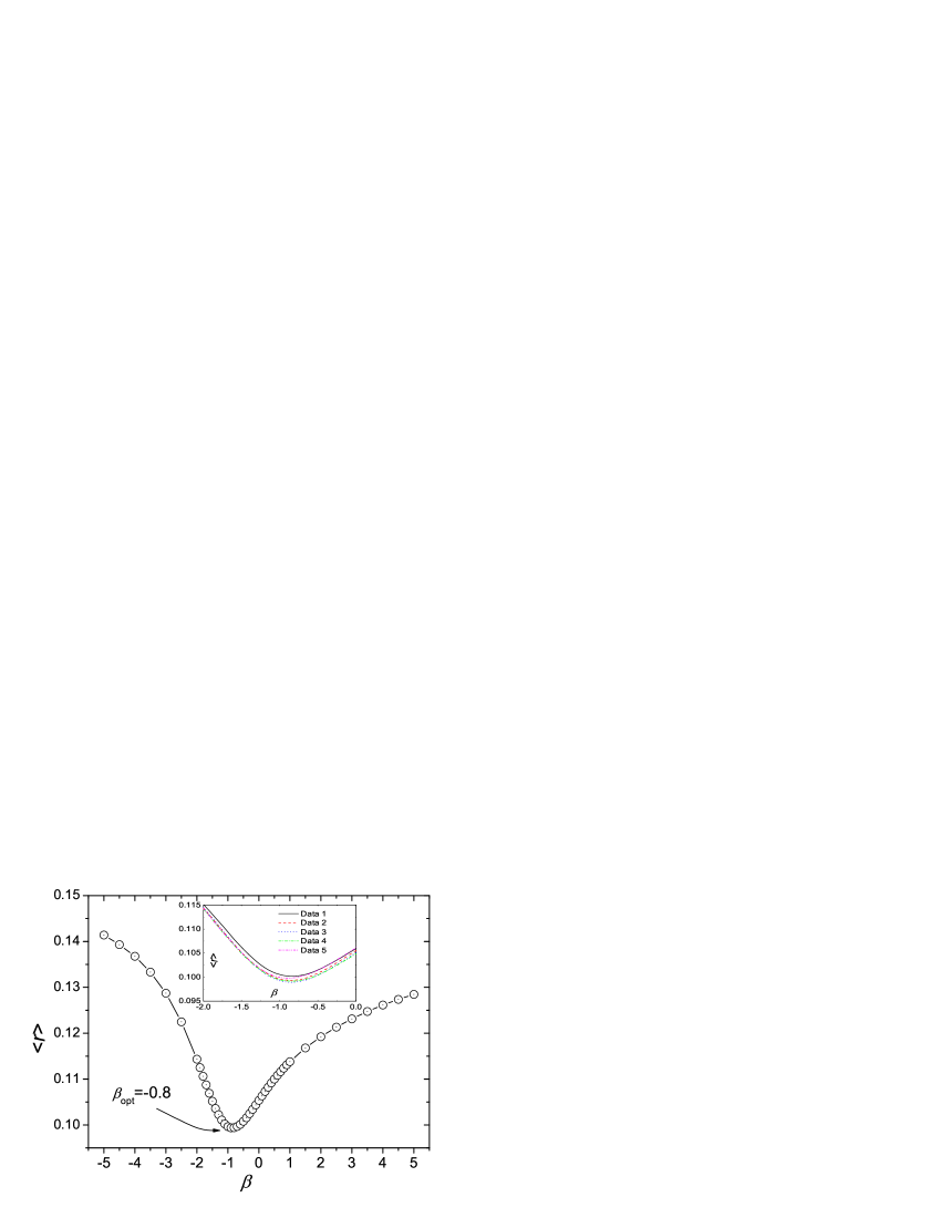
Figure 1: (Color online) The ranking score $\langle r\rangle$ vs. $\beta$. The optimal $\beta$, corresponding to the minimal $\langle r\rangle\approx 0.098$, is $\beta_{\texttt{opt}}\approx-0.8$. All the data points shown in the main plot is obtained by averaging over five independent runs with different data-set divisions. The inset shows the numerical results of every separate run, where each curve represents one random division of data-set.

Based on the user-object relations $A$, an object network can be constructed, where each node represents an object, and two objects are connected if and only if they have been collected simultaneously by at least one user. We assume a certain amount of resource (e.g. recommendation power) is associated with each object, and the weight $w_{ij}$ represents the proportion of the resource $o_{j}$ would like to distribute to $o_{i}$. For example, in the book-selling system, the weight $w_{ij}$ contributes to the strength of book $o_{i}$ recommendation to a customer provided he has bought book $o_{j}$. Following a network-based resource-allocation process where each object distributes its initial resource equally to all the users who have collected it, and then each user sends back what he/she has received to all the objects he/she has collected (also equally), the weight $w_{ij}$ (the fraction of initial resource $o_{j}$ eventually gives to $o_{i}$) can be expressed as:

$$w_{ij}=\frac{1}{k(o_{j})}\sum^{m}_{l=1}\frac{a_{il}a_{jl}}{k(u_{l})},$$ (1)

where $k(o_{j})=\sum^{n}_{i=1}a_{ji}$ and $k(u_{l})=\sum^{m}_{i=1}a_{il}$ denote the degrees of object $o_{j}$ and $u_{l}$, respectively. Clearly, the weight between two unconnected objects is zero. According to the definition of the weighted matrix $W=\{w_{ij}\}$, if the initial resource vector is $\mathbf{f}$, the final resource distribution is $\mathbf{f}^{\prime}=W\mathbf{f}$.

The general framework of the proposed network-based recommendation is as follows: (i) construct the weighted object network (i.e. determine the matrix $W$) from the known user-object relations; (ii) determine the initial resource vector $\mathbf{f}$ for each user; (iii) get the final resource distribution via $\mathbf{f}^{\prime}=W\mathbf{f}$; (iv) recommend those uncollected objects with highest final resource. Note that the initial configuration $\mathbf{f}$ is determined by the user’s personal information, thus for different users, the initial configuration is different. From now on, for a given user $u_{i}$, we use $\mathbf{f}^{i}$ to emphasize this personal configuration.

Numerical results. — For a given user $u_{i}$, the $j$th element of $\mathbf{f}^{i}$ should be zero if $a_{ji}=0$. That is to say, one should not put any recommendation power (i.e. resource) onto an uncollected object. The simplest case is to set a uniform initial configuration as

$$f^{i}_{j}=a_{ji}.$$ (2)

Under this configuration, all the objects collected by $u_{i}$ have the same recommendation power. In despite of its simplicity, it can outperform the two most widely applied recommendation algorithms, global ranking method (GRM) ex1 and collaborative filtering (CF) ex2 .

To test the algorithmic accuracy, we use a benchmark data-set, namely MovieLens ex3 . The data consists of 1682 movies (objects) and 943 users, and users vote movies using discrete ratings 1-5. We therefore applied a coarse-graining method similar to that used in Ref. Blattner2007 : a movie has been collected by a user if and only if the giving rating is at least 3 (i.e. the user at least likes this movie). The original data contains $10^{5}$ ratings, 85.25% of which are $\geq 3$, thus after coarse gaining the data contains 85250 user-object pairs. To test the recommendation algorithms, the data set is randomly divided into two parts: The training set contains 90% of the data, and the remaining 10% of data constitutes the probe. The training set is treated as known information, while no information in the probe set is allowed to be used for prediction.

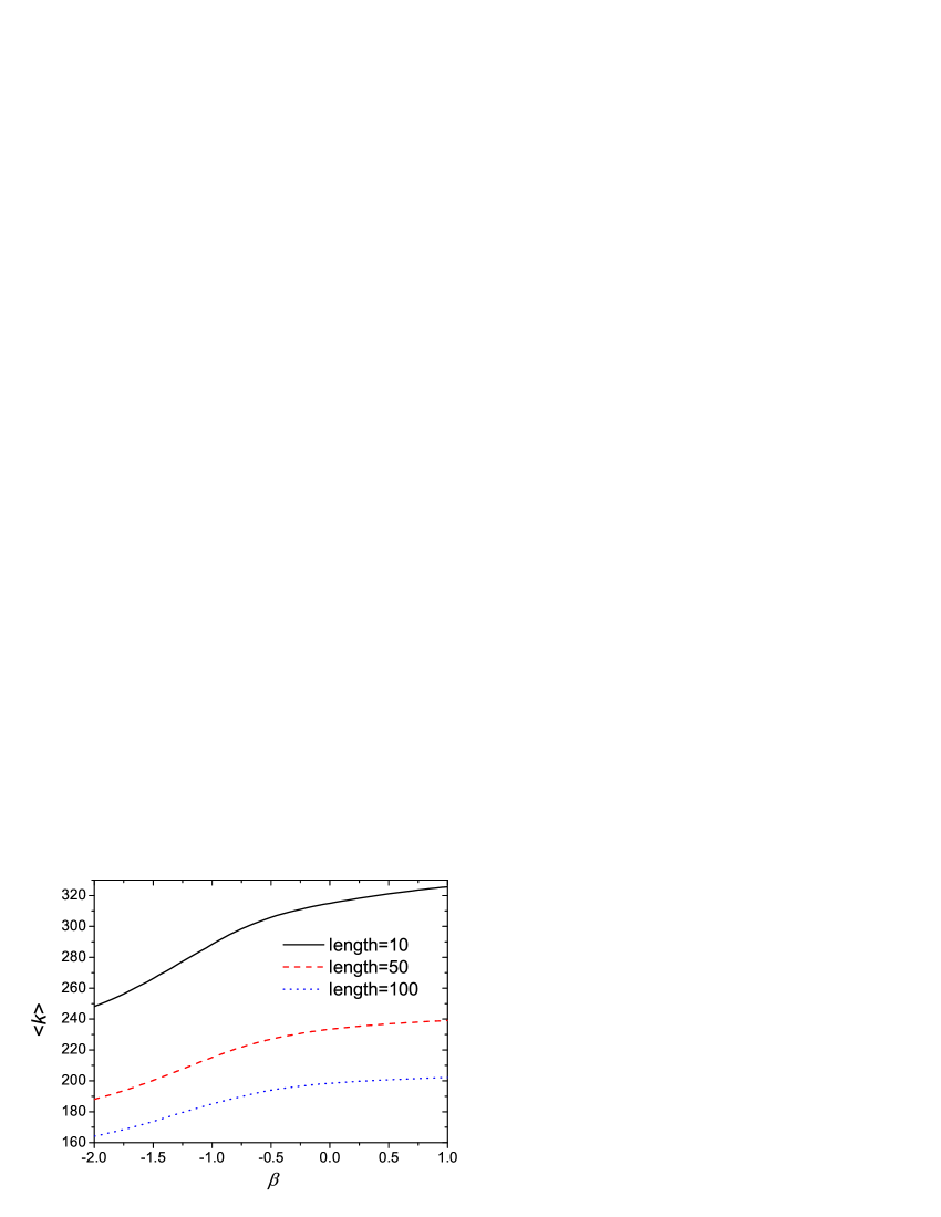
Figure 2: (Color online) The average degree of all recommended movies vs. $\beta$. The black solid, red dash and blue dot curves represent the cases with typical lengths $L=10$, 50 and 100, respectively. All the data points are obtained by averaging over five independent runs with different data-set divisions.

A recommendation algorithm should provide each user with an ordered queue of all its uncollected objects. For an arbitrary user $u_{i}$, if the relation $u_{i}-o_{j}$ is in the probe set (according to the training set, $o_{j}$ is an uncollected object for $u_{i}$), we measure the position of $o_{j}$ in the ordered queue. For example, if there are 1000 uncollected movies for $u_{i}$, and $o_{j}$ is the 10th from the top, we say the position of $o_{j}$ is 10/1000, denoted by $r_{ij}=0.01$. Since the probe entries are actually collected by users, a good algorithm is expected to give high recommendations to them, thus leading to small $r$. Therefore, the mean value of the position value $\langle r\rangle$ (called ranking score Zhou2007 ), averaged over all the entries in the probe, can be used to evaluate the algorithmic accuracy: the smaller the ranking score, the higher the algorithmic accuracy, and vice verse. Implementing the three algorithms mentioned above, the average values of ranking scores over five independent runs (one run here means an independently random division of data set) are 0.107, 0.122, and 0.140 for network-based recommendation, collaborative filtering, and global ranking method, respectively. Clearly, even under the simplest initial configuration, subject to the algorithmic accuracy, the network-based recommendation outperforms the other two algorithms.

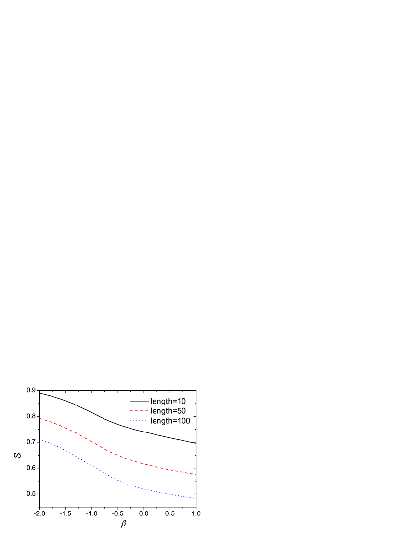
Figure 3: (Color online) $S$ vs. $\beta$. The black solid, red dash and blue dot curves represent the cases with typical lengths $L=10$, 50 and 100, respectively. All the data points are obtained by averaging over five independent runs with different data-set divisions.

Consider the initial resource located on object $o_{i}$ as its assigned recommendation power. In the whole recommendation process, the total power given to $o_{i}$ is $p_{i}=\sum_{j}f^{j}_{i}$, where the superscript $j$ runs over all the users $u_{j}$. Under uniform initial configuration (see Eq. (2)), the total power of $o_{i}$ is $p_{i}=\sum_{j}f^{j}_{i}=\sum_{j}a_{ij}=k(o_{i})$. That is to say, the total recommendation power assigned to an object is proportional to its degree, thus the impact of high-degree objects (e.g. popular movies) is enhanced. Although it already has a good algorithmic accuracy, this uniform configuration may be oversimplified, and depressing the impact of high-degree objects in an appropriate way could, perhaps, further improve the accuracy. Motivated by this, we propose a more complicated distribution of initial resource to replace Eq. (2):

$$f^{i}_{j}=a_{ji}k^{\beta}(o_{j}),$$ (3)

where $\beta$ is a tunable parameter. Compared with the uniform case, $\beta=0$, a positive $\beta$ strengthens the influence of large-degree objects, while a negative $\beta$ weakens the influence of large-degree objects. In particular, the case $\beta=-1$ corresponds to an identical allocation of recommendation power ($p_{i}=1$) for each object $o_{i}$.

Fig. 1 reports the algorithmic accuracy as a function of $\beta$. The curve has a clear minimum around $\beta=-0.8$. Compared with the uniform case, the ranking score can be further reduced by 9% at the optimal value. It is indeed a great improvement for recommendation algorithms. Note that $\beta_{\texttt{opt}}$ is close to -1, which indicates that the more homogeneous distribution of recommendation power among objects may lead to a more accurate prediction.

Besides accuracy, another significant ingredient one should take into account to for a personal recommendation algorithm is how personal this algorithm is. For example, suppose there are 10 perfect movies not yet known for user $u_{i}$, 8 of which are widely popular, while the other two fit a certain specific taste of $u_{i}$. An algorithm recommending the 8 popular movies is very nice for $u_{i}$, but he may feel even better about a recommendation list containing those two unpopular movies. Since there are countless channels to obtain information on popular movies (TV, the Internet, newspapers, radio, etc.), uncovering very specific preference, corresponding to unpopular objects, is much more significant than simply picking out what a user likes from the top of the list. To measure this factor, we go simultaneously in two directions. Firstly, given the length $L$ of recommendation list, the popularity can be measured directly by averaging the degree $\langle k\rangle$ over all the recommended objects. One can see from Fig. 2 that the average degree is positively correlated with $\beta$, thus depressing the recommendation power of high-degree objects gives more opportunity to unpopular objects. Also for $L=10$, 50 and 100, the corresponding $\langle k\rangle$ are 353.50, 258.00 and 214.09 (GRM), as well as 84.62, 87.95 and 83.79 (CF). Since GRM always recommends the most popular objects, it is clear that $\langle k\rangle_{\texttt{GRM}}$ is the largest. On the other hand, CF mainly depends the similarity between users. Thus one user may be recommended an object collected by another user having very similar habits to him, even though this object may be very unpopular. This is the reason why $\langle k\rangle_{\texttt{CF}}$ is the smallest. Secondly, one can measure the strength of personalization via the Hamming distance. If the overlapped number of objects in $u_{i}$ and $u_{j}$’s recommendation lists is $Q$, their Hamming distance is $H_{ij}=1-Q/L$. Generally speaking, a more personal recommendation list should have larger Hamming distances to other lists. Accordingly, we use the mean value of Hamming distance $S=\langle H_{ij}\rangle$, averaged over all the user-user pairs, to measure the strength of personalization. Fig. 3 plots $S$ vs. $\beta$ and, in accordance with the numerical results shown in Fig. 2, depressing the influence of high-degree objects makes the recommendations more personal. For $L=10$, 50 and 100, the corresponding $S$ are 0.508, 0.397 and 0.337 (GRM), as well as 0.654, 0.501 and 0.421 (CF). Note that, $S_{\texttt{GRM}}$ is obviously larger than zero, because the collected objects will not appear in the recommendation list, thus different users have different recommendation lists. Since CF has the potential to enhance the user-user similarity, $S_{\texttt{CF}}$ is remarkably smaller than that corresponding to negative $\beta$ in network-based recommendation.

In a word, without any increase in the algorithmic complexity, using an appropriate negative $\beta$ in our algorithm outperforms the uniform case (i.e. $\beta=0$) for all three criteria: more accurate, less popular, and more personalized.

Conclusions. — In this paper, we propose a recommendation algorithm based on a weighted object network. This algorithm is sensitive to the configuration of initial resource distribution. Even under the simplest case with binary resource, the current algorithm has remarkably higher accuracy than the widely applied GRM and CF. Since the computational complexity of this algorithm is much less than that of CF ex4 , it has great potential significance in practice. Furthermore, we introduce a free parameter $\beta$ to regulate the initial configuration of resource. Numerical results indicate that decreasing the initial resource located on popular objects further improves the algorithmic accuracy: In the optimal case ($\beta_{\texttt{opt}}\approx-0.8$), the distribution of total initial resource located on each object is very homogeneous ($p_{i}\sim k^{0.2}(o_{i})$). Besides the ranking score, there have been many measures suggested to evaluate the accuracy of personal recommendation algorithms Zhou2007 ; Billsus1998 ; Sarwar2000 ; Huang2004 , including hitting rate, precision, recall, F-measure, and so on. However, thus far, there has been no consideration of the degree of personalization. In this paper, we suggest two measures, $\langle k\rangle$ and $S$, to address this issue. We argue that to evaluate the performance of a recommendation algorithm, one should take into account not only the accuracy, but also the degree of personalization and popularity of recommended objects. Even under this more strict criterion, the case with $\beta_{\texttt{opt}}\approx-0.8$ outperforms the uniform case. Theoretical physics provides us some beautiful and powerful tools in dealing with this long-standing challenge in modern information science: how to do a personal recommendation. We believe the current work can enlighten readers in this interesting direction.

We acknowledge Runran Liu for very valuable discussion and comments on this work. This work is partially supported by SBF (Switzerland) for financial support through project C05.0148 (Physics of Risk), and the Swiss National Science Foundation (205120-113842). TZhou acknowledges NNSFC under Grant No. 10635040.

References

- (1) M. Faloutsos, P. Faloutsos, and C. Faloutsos, Comput. Comm. Rev. 29, 251 (1999).
- (2) A. Broder, et al., Comput. Netw. 33, 309 (2000).
- (3) G. Adomavicius, and A. Tuzhilin, IEEE Trans. Know. & Data Eng. 17, 734 (2005).
- (4) J. A. Konstan, B. N. Miller, D. Maltz, J. L. Herlocker, L. R. Gordon, and J. Riedl, Commun. ACM 40, 77 (1997).
- (5) J. L. Herlocker, J. A. Konstan, K. Terveen, and J. T. Riedl, ACM Trans. Inform. Syst. 22, 5 (2004).
- (6) M. Balabanović and Y. Shoham, Commun. ACM 40, 66 (1997).
- (7) M. J. Pazzani, Artif. Intell. Rev. 13, 393 (1999).
- (8) S. Maslov, and Y.-C. Zhang, Phys. Rev. Lett. 87, 248701 (2001).
- (9) K. Goldberg, T. Roeder, D. Gupta, and C. Perkins, Inf. Ret. 4, 133 (2001).
- (10) Y.-C. Zhang, M. Blattner, and Y.-K. Yu, Phys. Rev. Lett. 99, 154301 (2007).
- (11) T. Zhou, J. Ren, M. Medo, and Y.-C. Zhang, Phys. Rev. E 76, 046115 (2007).
- (12) Y.-C. Zhang, M. Medo, J. Ren, T. Zhou, T. Li, and F. Yang, EPL 80, 68003 (2007).
- (13) The global ranking method sorts all the objects in the descending order of degree and recommends those with highest degrees.
- (14) The collaborative filting is based on measuring the similarity between users. For two users and , their similarity can be simply determined by . For any user-object pair , if has not yet collected (i.e., ), the predicted score, (to what extent likes ), is given as . For any user , all the nonzero with are sorted in descending order, and those objects in the top are recommended.
- (15) The MovieLens data can be downloaded from the web-site of GroupLens Research (http://www.grouplens.org).
- (16) M. Blattner, Y. -C. Zhang, and S. Maslov, Physica A 373, 753 (2007).
- (17) Instead of calculating all the elements in , one can implement the current algorithm by directly diffusing the resource of each user. Ignoring the degree-degree correlation in user-object relations, the algorithmic complexity is , where and denote the average degree of users and objects. Correspondingly, the algorithmic complexity of collaborative filtering is , where the first term accounts for the calculation of similarity between users, and the second term accounts for the calculation of the predictions.
- (18) D. Billsus and M. J. Pazzani, Proc. 15th Int. Conf. Machine Learning, pp. 46-54 (1998).
- (19) B. Sarwar, G. Karypis, J. Konstan, and J. Riedl, Proc. ACM Conf. Electronic Commerce, pp. 158-167 (2000).
- (20) Z. Huang, H. Chen, and D. Zeng, ACM Trans. Inf. Syst. 22, 116 (2004).