Wave packet methods in cavity QED

Abstract

The Jaynes-Cummings model, with and without the rotating wave approximation, is expressed in the conjugate variable representation and solved numerically by wave packet propagation. Both cases are then cast into systems of two coupled harmonic oscillators, reminiscent of coupled bound electronic potential curves of diatomic molecules. Using the knowledge of such models, this approach of the problem gives new insight of the dynamics. The effect of the rotating wave approximation is discussed. The collapse-revival phenomenon is especially analyzed in a non-standard manner. Extensions of the method is briefly mentioned in terms of a three-level atom and the Dicke model.

1 Introduction

The main concepts of a wave packet approach to cavity quantum electrodynamics (QED) where put forward in [1]. The idea is to formulate the model Hamiltonian, either the Jaynes-Cummings (JC) model or the Rabi model [2, 3], in terms of the quadrature operators for the field rather than the commonly used boson ladder operators. The quadrature operators obey the regular conjugate commutator relations like position and momentum of a particle. As such, the problem can be viewed as a wave packet evolving on two coupled and bound potential curves (arising due to the two-level structure of the considered atom). The state of the system is, of course, embedded in the wave packet, where roughly speaking the potential curves determines the internal state of the two-level atom and the vibrational states of the wave packet correspond to the field mode state. Thus, once the wave packet is obtained any quantity is easily calculated. The JC and Rabi models are related through the rotating wave approximation (RWA) in which rapidly oscillating terms are neglected in the Rabi model to give the JC one. Correspondingly, the JC model is exactly solvable and the physical quantities of interest are in general represented by infinite sums deriving from the quantized nature of the cavity field. These analytical results are valid only in the regime where the RWA is justified, and beyond these the Rabi model must be considered. In the conjugate variable representation, both models exhibit an avoided crossing between the two potential curves, crucially affecting their dynamics. Surprisingly, especially around the avoided crossing the solvable JC model shows a non-intuitive wave packet dynamics, while the Rabi model display a more expected evolution.

In this paper we extend some of the results of [1] and describe how the method can be generalized to multi-level systems. Explicitly, we deepen the analysis about the phenomenon of collapse-revivals and discuss the differences in the evolution between the two models. The approach to collapse-revivals in the JC and Rabi models is somewhat different from the one typically used for wave packets evolution in molecular and chemical physics. This is thoroughly considered and the relation between the two viewpoints is sorted out. In particular, what is characterized by the revival time $T_{rev}$ for the JC model is labeled the classical period in wave packet dynamics. Thus, the time scale set by $T_{rev}$ can become very long compared to what one would expect from the classical period, which comes about due to the internal two-level structure of the model. Unlike [1], this paper briefly considers multi-level systems, that is when the number of internal states exceeds 2. We first consider a simple example of a three-level $\Lambda$-atom coupled to a single cavity mode, which serves as a prototype of how to extend the theory. More interesting is the following system of $N$ two-level atoms coupled to a quantized field, namely the Dicke model [4]. Here, the proper basis for the atomic subsystem is a collective one reminiscent of angular momentum states. Within this basis, the adiabatic diagonalization is straightforward and the $2^{N}$ potential curves are regained. An alternative approach is to use the Holstein-Primakoff representation [5], in which the $2^{N}$ atomic (fermionic) degrees of freedom is replaced by a single bosonic degree of freedom. In such case, the coupled potential curves are represented by one potential surface in 2-D.

We proceed as follows. In the next section 2 we introduce the model systems, the relation between the two models 2.1 is discussed and we give both models in the conjugate variable representation in 2.2. In this subsection we also mention how one may derive a semi-classical model that describes the population transfer between the two potential curves as the wave packet traverses the crossing. A deeper insight of the coupled dynamics is gained from the adiabatic representation, presented in 2.3. The following section 3 considers the non-intuitive evolution of the JC model compared to the Rabi model, while section 4 in detail studies the collapse-revival phenomenon, emphasizing on parallels between these two models and other wave packet systems. Section 5 is devoted to generalizations of the method to multi-level systems. Firstly, in 5.1 the idea is sketched using a simple three-level system, and in 5.2 we consider the Dicke model. Finally, section 6 gives a summary and outlooks.

2 The model system

2.1 Relation between the Rabi and the Jaynes-Cummings models

In most cavity QED experiments, their characteristics is well described by the Jaynes-Cummings model, in which single modes and atomic transitions are isolated and coherently coupled. This is achievable due to the strong atom-field coupling and the use of high-$Q$ cavities and long-lived atomic states, such that losses can be discarded over typical interaction periods. Within the dipole approximation, a microscopical derivation leads to the Rabi model defined by the Hamiltonian

$$H^{\prime}_{Rabi}=\hbar\omega\left(a^{\dagger}a+\frac{1}{2}\right)+\frac{\hbar\Omega^{\prime}}{2}\sigma_{z}+\hbar g^{\prime}_{0}\left(\sigma^{+}+\sigma^{-}\right)\left(a^{\dagger}+a\right).$$ (1)

Here, $a^{\dagger}$ ($a$) is the creation (annihilation) operator for the field mode; $a|n\rangle=\sqrt{n+1}|n+1\rangle$ ($a|n\rangle=\sqrt{n}|n-1\rangle$), the sigma operators are the standard Pauli matrices acting on the two-level atom; $\sigma_{z}|\pm\rangle=\pm|\pm\rangle$, $\sigma^{\pm}|\pm\rangle=|\mp\rangle$, $\sigma_{x}=\sigma^{+}+\sigma^{-}$ and $\sigma_{y}=-i\left(\sigma^{+}-\sigma^{-}\right)$, $\omega$ ($\Omega$) the field (atomic transition) frequency and $g^{\prime}_{0}$ is the effective atom-field coupling. Before proceeding, we define characteristic time and energy scales by $\omega^{-1}$ and $\hbar\omega$ respectively, and hence introduce the dimensionless variables $H_{Rabi}=H^{\prime}_{Rabi}/\hbar\omega$, $\Omega=\Omega^{\prime}/\omega$ and $g_{0}=g^{\prime}_{0}/\omega$. The interaction in (1) is built up from four terms; $\sigma^{+}a^{\dagger}$ and $\sigma^{-}a$ corresponding to simultaneous excitation/deaxcitation of the atom and the field, and $\sigma^{+}a$ and $a^{\dagger}\sigma^{-}$ originating from excitation of the atom by absorption of one photon and vice versa While the first terms are appropriately called non-energy conserving terms, the latter are termed energy conserving terms. In a rotating frame with respect to the first two terms of (1), the interaction constitutes precess with either the frequency $|\Omega+1|$ or $|\Omega-1|$, and provided

$$|\Omega-1|\ll|\Omega+1|$$ (2)

the rapidly oscillating terms may be left out. In this RWA limit, the Rabi Hamiltonian relaxes to the acclaimed Jaynes-Cummings model

$$H_{JC}=\left(a^{\dagger}a+\frac{1}{2}\right)+\frac{\hbar\Omega}{2}\sigma_{z}+\hbar g_{0}\left(\sigma^{+}a+\sigma^{-}a^{\dagger}\right).$$ (3)

The applicability of the RWA is not solely determined by the requirement (2), but also on the ratio $g_{0}/\Omega$. For large values of $g_{0}/\Omega$, the typical time scale of the interaction exceeds the one of free atomic evolution and the time-accumulated error arising from neglecting the non-energy conserving terms becomes important. Thus, apart from the condition (2) between the atomic transition and field frequencies, the validity of the RWA necessitates that $g_{0}<\Omega$ [6].

Given within the RWA, the number of excitations $N=a^{\dagger}a+\frac{1}{2}\sigma_{z}$ is a conserved quantity, and taking this symmetry into account the JC model is readily solvable with eigenstates

$$\begin{array}[]{l}\displaystyle{|E_{n}\rangle_{+}=\cos\left(\frac{\theta}{2}\right)|+,n-1\rangle+\sin\left(\frac{\theta}{2}\right)|-,n\rangle,}\\ \\ \displaystyle{|E_{n}\rangle_{-}=\sin\left(\frac{\theta}{2}\right)|+,n-1\rangle-\cos\left(\frac{\theta}{2}\right)|-,n\rangle,}\end{array}$$ (4)

where

$$\tan(2\theta)=\frac{2g_{0}\sqrt{n}}{\Delta}$$ (5)

and $\Delta=\Omega-1$. The corresponding eigenvalues read

$$E_{n}^{\pm}=\left(n+\frac{1}{2}\right)\pm\sqrt{\frac{\Delta^{2}}{4}+g_{0}^{2}n},$$ (6)

together with the uncoupled ground state $|E_{0}\rangle=|-,0\rangle$ with $E_{0}=-\Omega/2$.

2.2 Conjugate variable representation

The algebraic approach applied to the models presented in the previous section is, in many cases, preferable to other methods. In terms of the Rabi Hamiltonian, no exact analytical solutions exist and approximate concepts are developed to find the required quantities in certain parameter regimes [1]. For example, this enables for perturbation expansions or truncation of continued fraction solutions. Non the less, the validity of the results are restricted to specific parameters, and to go beyond these one must consider numerical approaches. The procedure used here adopts the $x$-representation in which the boson operators define the conjugate variables

$$p=i\frac{1}{\sqrt{2}}\left(a^{\dagger}-a\right),\hskip 28.45274ptx=\frac{1}{\sqrt{2}}\left(a^{\dagger}+a\right)$$ (7)

obeying $[x,p]=i$. In this representation, the Hamiltonians (1) and (3) become

$${H_{Rabi}=\frac{p^{2}}{2}+\frac{x^{2}}{2}+\left[\begin{array}[]{cc}\displaystyle{\frac{\Omega}{2}}&g_{0}\sqrt{2}x\\ g_{0}\sqrt{2}x&-\displaystyle{\frac{\Omega}{2}}\end{array}\right]},$$ (8)

$${H_{JC}=\frac{p^{2}}{2}+\frac{x^{2}}{2}+\left[\begin{array}[]{cc}\displaystyle{\frac{\Omega}{2}}&\displaystyle{\frac{g_{0}}{\sqrt{2}}\left(x+ip\right)}\\ \displaystyle{\frac{g_{0}}{\sqrt{2}}\left(x-ip\right)}&-\displaystyle{\frac{\Omega}{2}}\end{array}\right]}.$$ (9)

It is convenient to unitarily rotate $H_{Rabi}$ and $H_{JC}$ by $U=\frac{1}{\sqrt{2}}(\sigma_{x}+\sigma_{z})$ which gives the transformed Hamiltonians

$$\tilde{H}_{Rabi}=\frac{p^{2}}{2}+\left[\begin{array}[]{cc}V_{h}\left(x+\sqrt{2}g_{0}\right)&\displaystyle{\frac{\Omega}{2}}\\ \displaystyle{\frac{\Omega}{2}}&V_{h}\left(Q-\sqrt{2}g_{0}\right)\end{array}\right]-g_{0}^{2},$$ (10)

$$\tilde{H}_{JC}=\frac{p^{2}}{2}+\left[\begin{array}[]{cc}V_{h}\left(x+\displaystyle{\frac{g_{0}}{\sqrt{2}}}\right)&\displaystyle{\frac{\Omega}{2}-i\frac{g_{0}}{\sqrt{2}}p}\\ \displaystyle{\frac{\Omega}{2}+i{\frac{g_{0}}{\sqrt{2}}p}}&V_{h}\left(x-\displaystyle{\frac{g_{0}}{\sqrt{2}}}\right)\end{array}\right]-\frac{g_{0}^{2}}{4},$$ (11)

where $V_{h}(x)=x^{2}/2$. In the current nomenclature both models are identified as two displaced coupled harmonic oscillators, in which, however, the amount of displacement and the character of the couplings are emphatically different. For $x=0$ the two potential curves possess an avoided crossing and the dynamics around such degenrate points have been thoroughly analyzed in the studies of excited diatomic molecules [7]. Typically, the crucial part of the evolution occurs when the wave packet transverses an avoided crossing. To a good approximation the potentials can be linearized in the vicinity of the crossing. Considering the wave packet as a classical point particle following the classical equations of motion, the population transfer between the two levels while passing the crossing in the Rabi model can be estimated by the Landau-Zener formula [1, 8, 9]

$$P_{LZ}=1-\exp\left(-\frac{\sqrt{2}\pi\Omega^{2}}{8g_{0}v}\right).$$ (12)

Here $v$ is the classical velocity of the wave packet at the crossing, which, of course, depends on the initial state. Equation (12) directly gives some indicatives of the system behaviours; for a large velocity $v$ only a small fraction is transferred to the opposite state, and the same holds for a modest parameter $\Omega$ which couples the two levels. In order for the wave packet to bisect the crossing region, its initial mean position $x_{i}$ must satisfy $x_{i}<0$ or $x_{i}^{2}>2g_{0}^{2}$ for an initial state starting out “on” the right shifted oscillator or $x_{i}>0$ or $x_{i}^{2}<-2g_{0}^{2}$ for the left oscillator. For such a state, starting out on a single potential curve, a classical estimate of the velocity at the crossing gives $v\approx\sqrt{x_{i}^{2}-g_{0}^{2}/2}$. The evolutions is said to be adiabatic if $P_{LZ}\approx 1$, diabatic in the opposite limit and mesobatic in the intermediate regime. The same arguments applied to the JC model is considerably less direct as the two potential curves are coupled by a “momentum” dependent term. This term is the background to the aberrance between the two models in a most unexpected way. For $|\Omega|\gg g_{0}\sqrt{\bar{n}}$, where $\bar{n}$ is the average number of photons (directly related to the velocity $v$), it follows that the equations can be decoupled, which corresponds to adiabatic elimination of the two atomic internal states. This will be confirmed in the next subsection.

2.3 Adiabatic diagonalization

The previous section introduced the idea of potential curves associated with the Rabi and JC models, and the concept of adiabaticity became somewhat clear in this picture. Here we will stress this even further in order to gain a deeper understanding of the dynamics. As the JC model is exactly solvable we only carry out the analysis for the Rabi model.

The basis in which the Hamiltonian (8) is written might not be the most “optimal” one in the sense of decoupling the internal states. In most cases, the potential matrix describing the coupled dynamics has a smooth $x$-dependence, such that the characteristic length of derivative terms of the coupling elements decrease with the order of derivatives. A systematic way to remove the low-derivative terms from the off diagonals is by the adiabatic diagonalization. The unitary matrix $U_{1}$ that diagonalizates a the potential matrix for the Rabi model is given in (4) by replacing the angle; $\tan\left(2\theta\right)=2\sqrt{2}g_{0}x/\Omega$. From the identity

$$U_{1}^{\dagger}pU_{1}=p-\sigma_{y}\hbar\partial\theta,$$ (13)

where

$$\partial\theta\equiv\frac{\partial\theta}{\partial x}$$ (14)

it is clear that the transformed Hamiltonian is not diagonal. Explicitly we derive

$$\tilde{H}_{ad}=\frac{p^{2}}{2}+\frac{x^{2}}{2}+(\partial\theta)^{2}+\left[\begin{array}[]{cc}\lambda&\displaystyle{\frac{\partial^{2}\theta-2i(\partial\theta)p}{2}}\\ \displaystyle{\frac{\partial^{2}\theta-2i(\partial\theta)p}{2}}&-\lambda\end{array}\right],$$ (15)

where

$$\lambda=\sqrt{\frac{\Omega^{2}}{4}+2g_{0}^{2}x^{2}}$$ (16)

and

$$\partial\theta=\frac{\sqrt{2}\Omega g_{0}}{\Omega^{2}+8g_{0}^{2}x^{2}},\hskip 28.45274pt\partial^{2}\theta=-\frac{16\sqrt{2}\Omega g_{0}^{3}}{\left(\Omega^{2}+8g_{0}^{2}x^{2}\right)^{2}}.$$ (17)

The sizes of $\partial\theta$ and $\partial^{2}\theta$ measure the amount of adiabaticity [10, 11]. From these we can draw several conclusions; a large $\Omega$ favors an adiabatic evolution, so does a large $x$. The first is the regular adiabatic dispersive limit. The latter, however, is noticeably different from typical adiabaticicity in the JC model, but non the less it is intuitive since only close to the curve crossing is the adiabaticity assumed to break down. It seems that also $\Omega\rightarrow 0$ would give adiabatic evolution, which, however, is false since this limit describes the diabatic evolution. We recognize the adiabatic potentials

$$V_{ad}^{\pm}(x)=\frac{x^{2}}{2}+(\partial\theta(x))^{2}\pm\lambda(x)$$ (18)

and the internal adiabatic basis states as $|\uparrow\rangle=\cos(\theta)|+\rangle+\sin(\theta)|-\rangle$ and $|\downarrow\rangle=-\sin(\theta)|+\rangle+\cos(\theta)|-\rangle$. The internal diabatic basis states are termed $|u\rangle=\frac{1}{\sqrt{2}}(|+\rangle+|-\rangle)$ and $|d\rangle=\frac{1}{\sqrt{2}}(|+\rangle-|-\rangle)$, with corresponding diabatic potentials $V_{d}^{\pm}(x)=V_{h}(x\pm\sqrt{2}g_{0})$. Thus, a general adiabatic or diabatic state is is given by $\psi(x)|\uparrow(\downarrow)\rangle$ or $\psi(x)|u(d)\rangle$ respectively. Examples of the adibataic (solid) and diabatic (dotted) potentials are presented in figure 1.

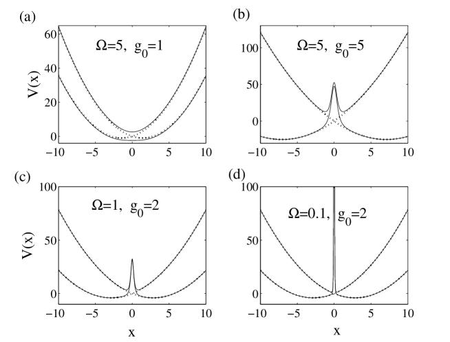
Figure 1: This figure displays different examples of the adiabatic potentials $V_{ad}^{\pm}(x)$ (solid lines) and diabatic potentials $V_{d}^{\pm}(x)$ (dotted lines).

Labeling $H_{ad}^{(1)}=H_{ad}=U_{1}HU_{1}^{\dagger}$, the transformed Hamiltonian $H_{ad}^{(1)}$ defines a new adiabatic diagonalization matrix $U_{2}$ and so forth, leading to the expansion $H_{ad}^{(n)}=\Big{[}U_{n}U_{n-1}\cdots U_{2}U_{1}\Big{]}H\Big{[}U_{1}^{\dagger}U_{2}^{\dagger}\cdots U_{n-1}^{\dagger}U_{n}^{\dagger}\Big{]}$. We further note that the rather general form of the adiabatic Hamiltonian (15) shares great similarities to the JC one (9) expressed in conjugate variables.

3 Regarding the $p$-dependent coupling

The presence of the $p$-dependent term in the potential matrix of the JC model (9), makes its evolution, in some sense, more complex (or less intuitive) than for its companion the Rabi model. On the one hand, we know that the JC model is analytically solvable and any physical quantity can in principle be obtained from certain infinite sums. Non the less, the fact remains that the wave packet dynamics is still more involved due to this term.

The analysis will be restricted to either initial Fock number, or coherent states, which in $x$-representations read respectively

$$\begin{array}[]{l}\displaystyle{\psi_{n}(x,0)=\frac{1}{\sqrt{2^{n}n!}}\left(\frac{1}{\pi}\right)^{1/4}\mathrm{H}_{n}(x)\mathrm{e}^{-\frac{x^{2}}{2}}},\\ \\ \displaystyle{\psi_{\nu}(x,0)=\left(\frac{1}{\pi}\right)^{1/4}\mathrm{e}^{-(\Im\nu)^{2}}\mathrm{e}^{-\frac{1}{2}\left(x-\sqrt{2}\nu\right)^{2}}},\end{array}$$ (19)

where $\mathrm{H}_{n}$ is the $n$th order Hermite polynomial and $\nu$ is the amplitude of the coherent state; $\bar{n}=|\nu|^{2}$. Thus, in the case of a coherent state, the classical velocity $v=\sqrt{2\bar{n}-g_{0}^{2}/2}$ at the crossing. For an initial Gaussian (19) centered at $x_{i}=0$, corresponding to field vacuum, one expects that the wave packet will split up and accelerate down towards the two potential minima [12]. This is indeed what we find for the Rabi model, while after all, this can not be the case for the JC model since we know that for an initial Fock state, the model exhibits Rabi oscillations. Thus, for the JC model the field wave packet will either Rabi oscillate between the two states $\psi_{0}(x)$ and $\psi_{1}(x)$ or remain in $\psi_{0}(x)$ throughout, whether the initial atomic state is $|+\rangle$ or $|-\rangle$. This constrain of the wave packet to the origin is a direct effect of the $p$-dependent coupling, and holds for any Fock state $\psi_{n}(x)$ and therefore also for Fock states extending over large ranges $x$. The wave packet must be considered in its entirety as a single object, or in other words the coherence extending over the whole wave packet must be taken into account and one can not incoherently split up the wave packet in separate individual pieces. From this fact, understanding the influence of the $p$-dependent coupling becomes more challenging. None the less, we have that for a $n$ photon Fock state $\Delta p^{2}=\langle p^{2}\rangle-\langle p\rangle^{2}=n+1/2$ and it is reasonable to expect that the ”momentum” coupling will affect the dynamics due to the large spread in $p$.

These conclusions are visualized in figure 2, which displays the squared absolute amplitude of the wave packet in the two models, together with the atomic inversion $\langle\sigma_{z}\rangle$. We use the split operator method [13] to obtain the wave packet

$$|\Psi(x,t)\rangle=\left[\begin{array}[]{c}\psi_{+}(x,t)\\ \psi_{-}(x,t)\end{array}\right],$$ (20)

and its squared absolute amplitude $P(x,t)=|\psi_{+}(x,t)|^{2}+|\psi_{-}(x,t)|^{2}$

Figure 2: The effect of the $p$-dependent coupling in the JC model. In the upper plot (a) we show the atomic inversion $\langle\sigma_{z}\rangle$ between the two internal atomic states $|\pm\rangle$ for the Rabi model (dashed) and the JC model (solid line) and the initial state is here; field in vacuum and the atom excited. The lower two plots presents the squared absolute amplitudes $P(x,t)$ of the wave packet in the Rabi (b) and JC (c) models. The parameters are $g_{0}=2$ and $\Omega=0.2$.

4 Collapse-revivals

Collapses of physical variables are caused by dephasing between the constitute terms making up the quantum state. While the collapses are expected, more surprising is the phenomenon of revivals, occurring when the terms return back in phase. Hence, the evolution must be sufficiently coherent in order to be able to complentate the rephasing. It is clear that revivals in the models considered in this paper is a direct outcome of the quantized ’grainyness’ of the field and thus a novel quantum effect [14]. In other fields, the existence of collapse-revivals has been greatly studied, and probably the most significant contribution owes the one of wave packet dynamics describing the vibrations in molecules [15]. Here the wave packet evolves in a bound electronic potential, where the discreteness derives from the vibrational eigen-modes in the particular electronic molecular state. For a harmonic potential, a wave packet bouncing back and forth in the potential, will reshape after one period of oscillation, which defines the classical period of motion. If the potential, however, is anharmonic the wave packet will not fully reshape after one classical period, bringing about the collapse. Depending on the degree of anharmonicity, the wave packet may reshape at later times characterizing the revivals. For a fairly localized excited wave packet, with average quantum number $\bar{n}\gg 1$, we assume $\Delta n/\bar{n}\ll 1$ where $\Delta n$ is the spread of quantum numbers. In this case we expand the eigenenergies accordingly,

$$E(n)=E(n_{0})+E^{\prime}(n_{0})(n-n_{0})+\frac{E^{\prime\prime}(n_{0})}{2}(n-n_{0})^{2}+\frac{E^{\prime\prime\prime}(n_{0})}{6}(n-n_{0})^{3}...\,,$$ (21)

where $E^{\prime}(n_{0})=(dE(n)/dn)_{n=n_{0}}$ and so on. The various terms define different time scales according to

$$\begin{array}[]{lll}T_{cl}=\frac{2\pi}{|E^{\prime}(n_{0})|},&T_{rev}=\frac{2\pi}{|E^{\prime\prime}(n_{0})|},&T_{sup}=\frac{2\pi}{|E^{\prime\prime\prime}(n_{0})|},\end{array}$$ (22)

characterizing classical, revival and superrevival times respectively. For a harmonic oscillator only the first of these term is non-zero and identifies the classical period $T_{cl}=2\pi/\omega$. We note that, assuming zero detuning, $\Delta=0$, the JC energies expand as $\sqrt{n}=\sqrt{\bar{n}}+\frac{1}{2\sqrt{\bar{n}}}(n-\bar{n})-\frac{1}{8\bar{n}^{3/2}}(n-\bar{n})^{2}+...\,$. This is not, however, the standard way of deriving the revival times in the JC model. Normally one solves for the time it takes for consecutive Rabi frequencies to differ by a multiple of $2\pi$

$$\left(2\Omega_{\bar{n}+1}-2\Omega_{\bar{n}}\right)T^{\prime}_{rev}=2\pi,$$ (23)

where $\Omega_{n}=\sqrt{\frac{\Delta^{2}}{4}+g_{0}^{2}n}$. The derived revival time is not identified with the previously defined $T_{rev}$ of equation (22), but rather associates with the classical time $T_{cl}$. In other words, $T_{cl}$ does not correspond to the time for the constitute wave packets to bounce back and forth in the potential. However, in the JC model, as well as in the Rabi model, one has two internal degrees of freedom, and the dynamics is obtained from both the internal wave packets and their coupled motion. In particular, reshaping of the wave packet means that both internal wave packets must reform simultaneously. Thus, using the definitions (22), $T_{cl}$ is typically orders of magnitude larger in a multi-level system than for an internal structure-less wave packet evolution. Another way of picturing the phenomenon is that the constitute wave packets must overlap in phase space in order to give rise to interference, manifesting itself in the form of revivals. By introducing $\langle x\rangle_{\pm}$ as the mean position of the two wave packets $\psi_{\pm}(x,t)$, and similarly for the momentum $\langle p\rangle_{\pm}$, revivals occur when $\delta x\equiv\langle x\rangle_{+}-\langle x\rangle_{-}=0$ and $\delta p\equiv\langle p\rangle_{+}-\langle p\rangle_{-}=0$ simultaneously. In figure 3 we show the atomic inversion and in figure 4 the quantities $\delta x$ and $\delta p$ as function of time $t$. In the $x$-direction, both models oscillates between $\pm 10$, while in the momentum direction the Rabi model has $\langle p\rangle$ exceeding 10 at some occasions.

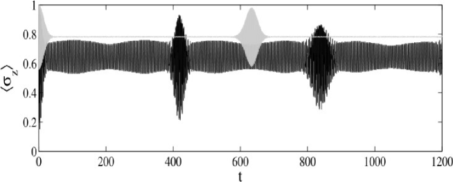
Figure 3: Inversion of the Rabi (black curve) and JC model (gray curve) for an initial coherent state with amplitude $\nu=7$, and dimensionless parameters $g_{0}=0.15$ and $\Omega=5$.

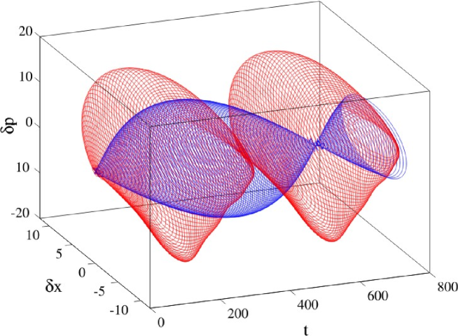
Figure 4: (Colour online) Inversion of the Rabi (red curve) and JC model (blue curve) for an initial coherent state with amplitude $\nu=7$, and dimensionless parameters $g_{0}=0.15$ and $\Omega=5$.

As argued, the revivals obtained in the Rabi and JC models correspond to the classical period $T_{cl}$ in equation (22), and not to $T_{rev}$ arising from the anharmonities. Due to the internal two-level structure, the time $T_{cl}$ can become rather long provided the proper adiabatic, diabatic or mesobatic potentials differ in their corresponding harmonic frequencies. However, if the frequencies almost coincide, $T_{cl}$ does not need to be large as seen in the example of figures 5 (atomic inversion) and 6 (wave packet amplitudes). Here the parameters are such that the evolution is approximately diabatic and the two Rabi diabatic potential curves share almost identical curvature, causing the two wave packets to oscillate with nearly the same classical frequencies. The JC model shows more abstract dynamics, more reminiscent of the one seen in figures 3 and 4.

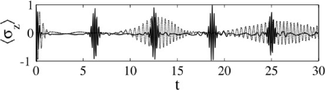
Figure 5: Inversion of the Rabi (solid line) and JC model (dotted line) for an initial coherent state with amplitude $\nu=4$, and dimensionless parameters $g_{0}=2$ and $\Omega=0.2$.

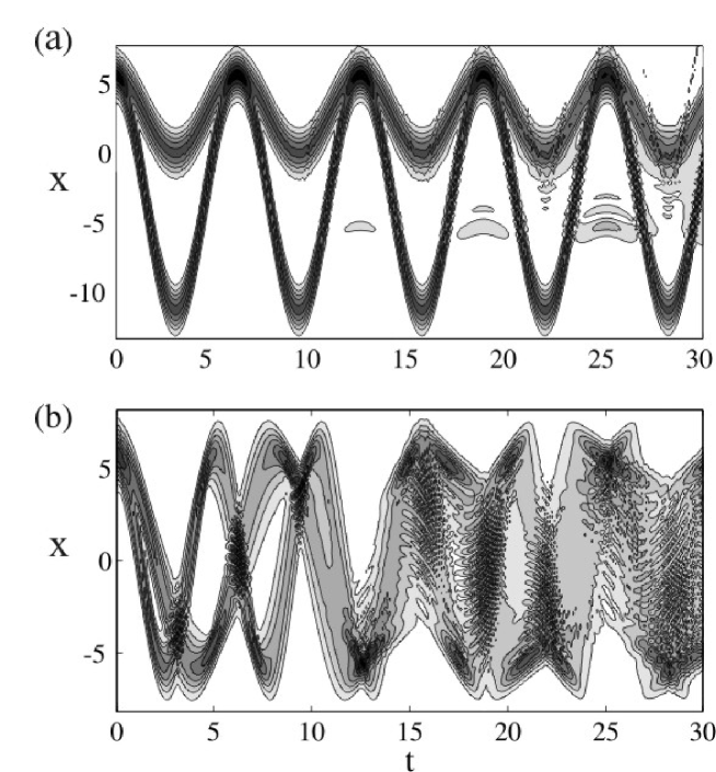
Figure 6: The squared amplitudes $P(x,t)$ for the Rabi (a) and the JC (b) models corresponding to fig. 5.

5 Extension to multi-level internal structure

In [1], the analysis was restricted to two-level atoms interacting with a single cavity mode. The generalization to multi-level atoms and/or multi-mode fields is straightforward. However, the split operator method can only handle up to two dimensions, limiting the numerics to at most two modes, while the number of internal states may be as large as 20. However, other approximate wave packet methods exists where the dimension might be considerably larger [16]. Here we only consider extensions in the direction of multi-level internal states, and the many mode situation will be dealt with in the future projects.

5.1 Three-level $\Lambda$-atom

In the regular two-level atom model, losses of the excited level often affects the dynamics in an undesired manner. This can be circumvented by coupling two metastable ”ground states” in a three-level $\Lambda$-atom configuration, adiabatically eliminating the excited state. However, the full three-level dynamics show interesting features beyond the two-level atom situation [17]. The model studied here is used mostly to present the methods, as it can in fact be reduced into a two-level model. Additionally, generalizing this model to non reducible three-level systems is straightforward.

For simplicity we assume the two lower atomic states, $|g_{1}\rangle$ and $|g_{2}\rangle$, to be degenerate, and further that they dipole couple to the excited state $|e\rangle$ through couplings $\lambda_{1}$ and $\lambda_{2}$. The Hamiltonian (without the RWA) reads

$$H_{\Lambda}=\frac{p^{2}}{2}+\frac{x^{2}}{2}+\Omega\sigma_{ee}+\big{[}\lambda_{1}\left(\sigma_{g_{1}e}+\sigma_{eg_{1}}\right)+\lambda_{2}\left(\sigma_{g_{2}e}+\sigma_{eg_{2}}\right)\big{]}x,$$ (24)

where $\sigma_{ij}=|i\rangle\langle j|$. It may be written in the atomic bare basis $\left\{|g_{1}\rangle,|e\rangle,|g_{2}\rangle\right\}$ as

$$H_{\Lambda}=\frac{p^{2}}{2}+\frac{x^{2}}{2}+\left[\begin{array}[]{ccc}0&\lambda_{1}x&0\\ \lambda_{1}x&\Omega&\lambda_{2}x\\ 0&\lambda_{2}x&0\end{array}\right].$$ (25)

Introducing the angles $\tan(\theta)=\lambda_{1}/\lambda_{2}$ and $\tan(2\phi)=2\lambda_{0}x/\Omega$, with $\lambda_{0}=\sqrt{\lambda_{1}^{2}+\lambda_{2}^{2}}$, the potential matrix is diagonalized by

$$U_{2}=\left[\begin{array}[]{ccc}\sin(\phi)\sin(\theta)&\cos(\theta)&\cos(\phi)\sin(\theta)\\ \cos(\phi)&0&-\sin(\phi)\\ \sin(\phi)\cos(\theta)&-\sin(\theta)&\cos(\phi)\cos(\theta)\end{array}\right].$$ (26)

As $\theta$ is $x$-independent we find

$$U_{2}pU_{2}^{\dagger}=p-iU_{2}\partial_{\phi}U_{2}^{\dagger}\partial_{x}\phi,$$ (27)

and one derives that

$$U\partial_{\phi}U^{\dagger}=\left[\begin{array}[]{ccc}0&0&1\\ 0&1&0\\ 1&0&0\end{array}\right].$$ (28)

The adiabatic potentials are

$$V_{\pm}(x)=\frac{x^{2}}{2}+(\partial_{x}\phi)^{2}+\left(\frac{\Omega}{2}\pm\sqrt{\frac{\Omega^{2}}{4}+2\lambda_{2}^{2}x^{2}}\right),\hskip 34.14322ptV_{0}(x)=\frac{x^{2}}{2}+(\partial_{x}\phi)^{2},$$ (29)

where the adiabatic state corresponding to $V_{0}(x)$ is called the dark state which becomes degenerate with the state of $V_{-}(x)$ at $x=0$. This degeneracy is lifted however, if a detuning is assumed between the two ground states. We note that the two adiabatic potentials $V_{\pm}(x)$ are similar to the ones of the Rabi model (18). Actually, the absence of a second non-zero diagonal element in the potential matrix gives the system a symmetry such that it can be separated into a $2\times 2$ problem. The unitary transformation

$$U_{3}=\frac{1}{\lambda_{0}}\left[\begin{array}[]{ccc}\lambda_{1}&0&\lambda_{2}\\ 0&\lambda_{0}&0\\ \lambda_{2}&0&-\lambda_{2}\end{array}\right]$$ (30)

casts the potential matrix in the form

$$V^{\prime}(x)=U_{3}V(x)U_{3}^{\dagger}=\left[\begin{array}[]{ccc}0&\lambda_{0}x&0\\ \lambda_{0}x&\Omega&0\\ 0&0&0\end{array}\right].$$ (31)

We may remark that like for the Rabi model, a semiclassical approach of this $\Lambda$-system naturally leads to the solvable generalized three-level Landau-Zener model [18]. Wave packet propagation methods in a related system has been considered in [19].

5.2 Dicke model

Extending the Rabi Hamiltonian to contain $N$ number of two-level atoms gives the Dicke model [4]

$$H_{D}=\frac{p^{2}}{2}+\frac{x^{2}}{2}+\Omega S_{x}+\frac{g_{0}}{\sqrt{N}}S_{z}x$$ (32)

with the total spin observables $S_{k}=\sum_{i=1}^{N}\sigma_{k}^{(i)}$, $k=x,z$ and $\sigma_{k}^{(i)}$ is the $k$’th Pauli matrix for atom $i$. The scaling of the atom-field coupling by $\sqrt{N}$ is inserted to assure a well defined thermodynamic limit as $N\rightarrow\infty$. Operators acting on different atoms commutes, so that the adiabatic atomic ground state reads

$$|E_{0}\rangle=\big{\{}\cos(\theta)|+\rangle-\sin(\theta)|-\rangle\big{\}}^{\otimes N},$$ (33)

where $\otimes N$ means direct product and as before $\tan(2\theta)=2g_{0}x/\sqrt{N}\Omega$. Formally, the adiabatic diagonalization procedure follows like for the single atom case, replacing Pauli matrices by total spin operators. We unitary transform the Hamiltonian by

$$U_{4}=\mathrm{e}^{-i\theta S_{y}}$$ (34)

and the non-adiabatic corrections arise from equation (13) substituting $\sigma_{y}$ by $S_{y}$. From the theory of angular momentum we directly find the adiabatic potentials

$$V_{m_{s}}(x)=\frac{x^{2}}{2}+m_{s}\sqrt{\frac{\Omega^{2}}{4}+\frac{g_{0}^{2}}{N}x^{2}},\hskip 34.14322ptm_{s}=-N,-N+1,...,N-1,N.$$ (35)

Here $m_{s}$ is the quantum number for the total spin in the $z$-direction. It is convenient to introduce the Dicke states $|s,m_{s}\rangle$ being eigenstates of the total spin $S|s,m_{s}\rangle=s(s+1)|s,m_{s}\rangle$ and of the $z$-component $S_{z}|s,m_{s}\rangle=m_{s}|s,m_{s}\rangle$. The adiabatic ground state thus identifies with quantum numbers $s=N$ and $m_{s}=-N$, and applying the rotated annihilation operator $\tilde{J}_{+}=U_{4}^{\dagger}J_{+}U_{4}$ repeated times to the ground state generates all the adiabatic states $|N,m_{s}\rangle$. The states with lower $s$ quantum number can be obtained by standard methods.

In the large $N$ limit, quantum fluctuations can in general be regarded as small and one may linearize these terms. The Holstein-Primakoff representation of the spin operators [5] has turned out to be an efficient approach in analyzing the Dicke model [20, 21]. The spin operators are expressed in boson operators accordingly;

$$S_{z}=b^{\dagger}b.\frac{N}{2},\hskip 28.45274ptS_{+}=b^{\dagger}\sqrt{N-b^{\dagger}b},\hskip 28.45274ptS_{-}=S_{+}^{\dagger}.$$ (36)

Before linearizing, we note from figure 1 that the low lying adiabatic potentials (we assume cold atoms and therefore a low temperature) either have one or two global minima, and this fact should be taken into account for when expanding in $N^{-1}$. This is directly related to the presence of a quantum phase transition, with critical coupling $g_{0}^{(c)}=\sqrt{\Omega}/2$, between the normal phase of a vacuum field and all atoms deexcited and the superradient phase of a macroscopic field and atomic excitation [22, 23]. Due to this it is convenient to coherently shift the boson operators as [20, 21]

$$a\rightarrow c+\alpha_{s},\hskip 34.14322ptb\rightarrow d+\beta_{s},$$ (37)

where

$$\alpha_{s}=g_{0}\sqrt{N(1-\mu^{2})},\hskip 34.14322pt\beta_{s}=\sqrt{\frac{N}{2}(1-\mu)}$$ (38)

and

$$\mu=\left\{\begin{array}[]{llll}\left(\frac{g_{0}^{(c)}}{g_{0}^{2}}\right)^{2},&&g_{0}>g_{0}^{(c)}\\ 1,&&g_{0}\leq g_{0}^{(c)}\end{array}\right..$$ (39)

Thus, we note that in the case of a single global minimum the shifts vanish. Here $c$ and $d$ represents quantum fluctuations around the classical values $\alpha_{s}$ and $\beta_{s}$. The resulting expanded Dicke Hamiltonian becomes [20, 21]

$$H_{D}^{\prime}=c^{\dagger}c+\frac{\Omega(1+\mu)}{2\mu}d^{\dagger}d+\frac{\Omega(1-\mu)(3+\mu)}{8\mu(1+\mu)}(d^{\dagger}+d)^{2}+g_{0}\mu\sqrt{\frac{2}{1+\mu}}(c^{\dagger}+c)(d^{\dagger}+d).$$ (40)

For $\mu=1$ (the ground adiabatic potential possess only a single minimum) the Hamiltonian becomes bi-linear and one may decouple the two boson modes into two disconnected harmonic oscillators.

Using the Holstein-Primakoff representation we turn the fermionic degrees of freedom into a single bosonic degree of freedom. The cost of reducing the $2^{N}$ potential curves to a single one is that the wave packet now evolves in 2-D rather than 1-D. Non the less, wave packet propagation in 2-D is easily performed with the split operator method, and will be consider in future works. Another algebraic method that could be considered is the ”Schwinger’s oscillator model of angular momentum” [24], in which, however, two bosonic degrees of freedom is introduced instead of the fermionic subsystem.

6 Conclusion

The method of wave packet propagation, in which the cavity fields quadrature operators serve as conjugate variables, has been explored. It has been applied to the seminal JC model and its companion, the Rabi model, which is related to the JC one by the RWA. Various bases, different form the conventional bare and dressed bases, and their corresponding potential curves were consider. This new numerical approach is more commonly used in chemical and molecular physics, were it has been utilized for more than three decades [25]. The effect of the RWA was discussed in this representation, and rather unexpected phenomena of the wave packet evolution appear once the RWA has been assumed.

The main part of the analysis has been devoted to the collapse-revival effect of these models. Typically it is studied using algebraic methods, while we examine it from the shapes of the coupled potential curves. The terminology of collapse-revivals in wave packet models is not the same as the one for the JC model and we sort this out. The internal two-level structure of the Rabi and JC models may cause very long characteristic time scales, compared to the ones of a wave packet in a single anharmonic potential.

Finally we have sketched how the method is extended to systems with more internal degrees of freedom, and here especially to the three-level $\Lambda$-atom and the Dicke model. For the Dicke model, we show how one may transform the internal degrees of freedom into a single ”external” degree of freedom using the Holstein-Primakoff representation. More thorough research on multi-level and multi-mode systems are left for future works.

The author acknowledges support from the Swedish government/Vetenskapsrådet and the European Commission (EMALI, MRTN-CT-2006-035369; SCALA, Contract No. 015714).

References

References

- [1] Larson J 2007 Phys. Scr. 76 146.
- [2] Jaynes E T and Cummings F W 1963 Proc. IEEE 51 89
- [3] Rabi I I 1926 Phys. Rev. 49 324
- [4] Dicke R H 1954 Phys. Rev. 93 99
- [5] Holstein T and Primakoff H 1940 Phys. Rev. 58 1098
- [6] The effective atom-field coupling scales as and therefore this conditiond modifies to , where is the average number of photons.
- [7] Garraway B M and Suominen K A 1995 Rep. Prog. Phys. 58 365
- [8] Landau L D 1932 Sowjet Union 2 46
- [9] Zener C 1932 Proc. R. Soc. 137 696
- [10] Larson J and Stenholm S 2006 Phys. Rev. A 73 033805
- [11] Note that, apart from the derivative terms and , the “momentum” enters in the off-diagonal elements of (15) in agreement with the conclusions of subsection 2.2.
- [12] Here we have assumed paramteres such that the lower adiabatic potential pocesses two minima.
- [13] Fleit M D, Fleck J A and Steiger A 1982 J. Comput. Phys. 47, 412
- [14] Eberly J H, Narozhny N B and Sanchez-Mondragon J J 1980 Phys. Rev. Lett. 44 1323
- [15] Robinett R W 2004 Phys. Rep. 392 1
- [16] http://www.pci.uni-heidelberg.de/tc/usr/,ctdh/
- [17] Messina A, Maniscalco S and Napoli A 2003 J. Mod. Opt. 50 1
- [18] Carroll C E and Hioe F T 1986 J. Phys. A: Math. Gen. 19 2061
- [19] Larson J 2006 Phys. Rev. A 73 013823
- [20] Emary C and Brandes T 2003 Phys. Rev. Lett 90 044101
- [21] Emary C and Brandes T 2003 Phys. Rev. E 67 066203
- [22] Hepp K and Lieb E H 1973 Ann. Phys. 76 360
- [23] Wang Y K and Hioe F T 1973 Phys. Rev. A 7 831
- [24] Sakurai J J 1995 Modern Quantum Mechanics (Addison-Wesley)
- [25] Heller E J 1975 J. Chem. Phys. 62 1544