Open Inflationary Universes in Gauss-Bonnet Brane Cosmology

Abstract

In this article, we study a type of one-field approach for open inflationary universe scenario in the context of braneworld models with a Gauss-Bonnet correction term. For a one-bubble universe model, we determine and characterize the existence of the Coleman-De Lucia instanton together with the period of inflation after tunneling has occurred. Our results are compared those analogous obtained when the usual Einstein Theory of Gravitation is used.

I Introduction

Recent observations from the WMAP wmap are entirely consistent with a universe have a total energy density that is very close to its critical value, where the total density parameter has the value $\Omega=1.02\pm 0.04$. Most people interpret this value as corresponding to a flat universe. But, according to this result, we might take the alternative point of view of have a marginally open or close universe model ellis-k , which early presents an inflationary period of expansion. At this point, we should mention that Ratra and Peebles were the first to elaborate on the open inflation model Ratra ; Ratra2 . The approach of consider open or a closed inlfationary universe models has already been considered in the literature, re6 ; re8 ; shiba ; ramon ; delCampo:2004gh ; del Campo:2004ee ; Balart:2007je in the context of the Einstein theory of relativity, Jordan-Brans-Dicke (JBD) theory, Randall-Sundrum type of gravitation theory, and tachyonic field cosmology respectively. All these models have been worked out in a four dimensional spacetime or on a four dimensional brane (where lived matter contents) embedding in a five dimensional bulk. The idea of considering an extra dimension has received great attention in the last few years, since it is believed that these models shed light on the solution to fundamental problems when the universe is traced back to very early times. Specifically, the possibility of creating an open or closed universe from the context of a Brane World (BW) scenario MBPGD ; MBPGD2 ; MBPGD3 , has quite recently been considered.

BW cosmology offers a novel approach to our understanding of the evolution of the universe. The most spectacular consequence of this scenario is the modification of the Friedmann equation, in a particular case when a five dimensional model is considered, and where the matter described through a scalar field, is confined to a four dimensional Brane, while gravity can be propagated in the bulk. These kind of models can be obtained from superstring theory witten ; witten2 . For a comprehensible review on BW cosmology, see Refs. lecturer ; lecturer2 ; lecturer3 for example. Specifically, consequences of a chaotic inflationary universe scenario in a BW model was described maartens , where it was found that the slow-roll approximation is enhanced by the modification of the Friedman equation.

When a stage closed to the Big-Bang is studied, quantum effects should be included in the bulk. In the high dimensional theory, the high curvature correction terms should be added to the Einstein Hilbert action. As far as it is well known, the correction term does not introduce ghost in this action is the Gauss-Bonnet (GB) combination. The GB term arises naturally as the leading order of the $\alpha^{\prime}$ expansion of heterotic superstring theory, where, $\alpha^{\prime}$ is the inverse string tension. The GB term is given by

$$GB=R^{\mu\nu\lambda\rho}R_{{}^{\mu\nu\lambda\rho}}-4R^{\mu\nu}R_{\nu\mu}+R^{2},$$ (1)

that often appears in higher dimensional version of gravity theories, especially in string theory. In fact, all versions of string theory (except Type II) in 10 dimensions (D = 10) include this term. Therefore, could be interesting to make an study of the effects of the Gauss-Bonnet term that produces on inflationary braneworld models Meng:2003pn ; Lidsey:2003sj ; Calcagni:2004as ; Kim:2004gs ; Kim:2004jc ; Kim:2004hu ; Murray:2006fw . On the other hand, Gauss-Bonnet term was consider as an alternative for explain the mysterious of currently dark energy observedLeith:2007bu ; Koivisto:2006ai ; Sanyal:2006wi ; Koivisto:2006xf ; Carter:2005fu ; Nojiri:2005am ; Nojiri:2005vv . The purpose of the present paper is to study an open inflation universe model, where the scalar field is confined to the four dimensional Brane that is embedded in five dimensional bulk where a Gauss-Bonnet (GB) contribution is considered.

The plan of the paper is as follows: In Sec. II we specify the effective four dimensional cosmological equations from a five-Anti de Sitter GB brane world model. We write down the Euclidean field equations, and then we solve them numerically. Here, the existence of the Coleman-De Lucia (CDL) instanton is established. In Sec. III we determine the characteristics of an open inflationary universe model that is produced after tunneling process has occurred. Our results are compared to those analogous results obtained by using Einstein’s theory of gravity. Finally, we conclude in Sec. IV.

II The Euclidean cosmological equations in Randall-Sundrum type II Scenario

We start with the action given by

$$S = \frac{1}{2\kappa_{5}^{2}}\int_{bulk}d^{5}x\sqrt{-g_{5}}\left\{R-2\Lambda_{5}+\alpha\left(R^{\mu\nu\lambda\rho}R_{{}^{\mu\nu\lambda\rho}}-4R^{\mu\nu}R_{\nu\mu}+R^{2}\right)\right\},$$ (2)

$$+\int_{brane}d^{4}x\sqrt{-g_{4}}\left(\mathcal{L}_{matter}-\lambda\right),$$

where $\Lambda_{5}=-3\mu^{2}\left(2-4\alpha\mu^{2}\right)$ is the cosmological constant in five dimensions, with the $AdS_{5}$ energy scale $\mu=1/l$ and $\lambda$ corresponds to the brane tension. $\mathcal{L}_{matter}$ is the matter lagrangian for the inflaton field on the brane. $\kappa_{5}^{2}=8\pi/m_{5}$ is the five dimensional gravitational coupling constant. Finally, the GB coupling constant $\alpha$ can be related to the string scale ($g_{s}$) as $\alpha\simeq 1/8g_{s}$ when the GB term is taken as to the lowest-order stringy correction to the 5D gravity. Cosmological dynamics on the brane arise due to its motion through the static bulk space. If we consider a Friedmann-Robertson-Walker brane, where the scale factor $a(t)$ describes the position of the brane in the bulk. The exact Friedmann-like equation is given by davis

$$2\mu\sqrt{1+\frac{H^{2}}{\mu^{2}}}\left(3-4\alpha\mu^{2}+8\alpha H^{2}\right)+\frac{k}{a^{2}}=\kappa_{5}^{2}\left(\rho+\lambda\right),$$ (3)

where $\rho$ represents the energy density of the matter sources on the brane and $k=0,+1and-1$ represents flat,closed and open spatial section, respectively. The conservation equation of the matter onto the brane follows directly from Gauss-Codazzi equations. For a perfect fluid matter source, it is reduced to the familiar form,

$$\dot{\rho}+3H\left(\rho+p\right)=0.$$ (4)

In term of the inflaton field Eq.(4) can be written as

$$\ddot{\phi}+3\frac{\dot{a}}{a}\dot{\phi}+V_{,\phi}(\phi)=0\,\,,$$ (5)

where $V(\phi)$ represents the effective potential associated to the inflaton field. This potential is given by

$$V(\phi)=\frac{1}{2}m^{2}\left(1+\frac{\alpha^{2}}{\delta^{2}+(\phi-v)^{2}}\right),$$ (6)

where $\alpha$, $\delta$ and $v$ are arbitrary constants, which will be set by phenomenological considerations. This potential was first considered by Lindere6 in order to obtain a successful scenario for open inflation in Einstein’s. The first term of the effective potential controls inflation after quantum tunnelling has occurred (its shape coincides with that used in the simplest chaotic inflationary universe model, $m^{2}\phi{{}^{2}}/2$), and the second term controls the bubble nucleation, whose role is to create an appropriate shape in the inflaton potential, $V(\phi)$ .i.e., the parameters $\alpha$, $\delta$ and $v$ just affect the quantum tunelling process. Therefore, once that tunelling occurs the inflationary dynamics is drives by the simplest chaotic potential and the parameters of the second term are not considering in the inflationary epoch. Following Ref. ramon we take $\delta^{2}=0.1$, $\delta^{2}=2\alpha^{2}$, and $v=3.5$, which, will provide the adequate N e-folds number of inflation after the tunneling. Certainly, this is not the only choice, since other values for these parameters can also lead to a successful open inflationary scenario (with any value of $\Omega$, in the range $0<\Omega<1$).

In particular, in our model the Gauss Bonnet Brane World the inflaton field begins at the false vacuum ($\phi_{F}$) and then decays to the value $\phi_{T}$ via quantum tunnelling through the potential barrier (see Fig.1), generating during this process an open inflationary universe. In order to study the nucleation of bubble we write down the corresponding Euclidean equations of motion, and the $O(4)$ invariant Euclidean spacetime metric is written as

$$d{s}^{2}\,=\,d{\tau}^{2}\,+\,a(\tau)^{2}\,(\,\,d{\psi}^{2}\,+\,\sin^{2}\psi\,d{\Omega_{2}^{2}}\,\,).$$ (7)

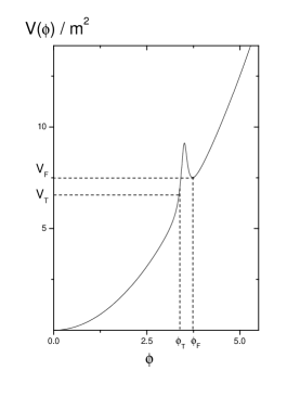
Figure 1: The potential form for the inflaton field, as in Ref. re6 , we will consider the theory with $m=1.5\times 10^{-6}$, which is necessary to have a proper amplitude for density perturbations during inflation in the model with $q=1$. And $v=3.5$, which, will provide the adequate N e-folds number of inflation after the tunneling. By changing this parameter by few percent one can get any value of $\Omega$ from 0 to 1. In particular we will take $\delta^{2}=2\alpha^{2}$ with $\delta=0.1$.

Instead of using the complicated form for the exact Friedmann-like equation (3), we used an effective Friedmann equation given by

$$H^{2}-\frac{1}{a^{2}}=\beta_{q}^{2}\rho^{q},$$ (8)

where $\beta_{q}^{2}$ is a model dependent constant, whose values are justified for the observation (in particular for the values of N e-folds number after inflations and for the density of scalar perturbations).

Table 1: This table shows the values of $\beta$ in Eistein-Hilbert and Gauss Bonnet Brane world models.

Model	$q$	$\beta_{q}$
Einstein Hilbert	$1$	$10$
Gauss Bonnet Brane World	$2/3$	$10^{-3}$

Then, we can written the Euclidean field equations as follow,

$$a^{\prime\prime} = -a\beta_{q}m^{2\left(q-1\right)}\left(-\frac{\phi^{\prime 2}}{2}+V(\phi)\right)^{q}\left[1+\frac{3}{2}q\frac{\phi^{\prime 2}}{\left(-\frac{\phi^{\prime 2}}{2}+V(\phi)\right)}\right],$$ (11)

$$\begin{array}[]{ll}&\phi^{\prime\prime}+3\frac{a^{\prime}}{a}\phi^{\prime}-V_{,\phi}=0,\end{array}$$

where the upper prime represent derivative with respect to Euclidean time ($\tau$) and $V_{,\phi}=\frac{dV}{d\phi}$.

We have solved numerically the field equations (11) for the values gives in table I in the effective Friedmann equation  (8). The boundary conditions that we have used were those in which $\phi^{\prime}=0$ and $a^{\prime}=1$ at $a=0$. On the other hand, we take $m\simeq 10^{-6}$ and the value of the constant $\delta$ is chosen in such a way that an appropriate amplitude for density perturbations is obtained. We have also taken the value $v=3.51$ since they provide the needed $65$ e-folds of inflations after tunneling has occurred. At $\tau\approx 0$, the scalar field $\phi=\phi_{T}$ lies in the true vacuum, near the maximum of the scalar potential $V(\phi)$. At $\tau\neq 0$, the same field is found close to the false vacuum, but now with a different value, $\phi=\phi_{F}$. Specifically, the scalar field $\phi$ evolves from some initial value $\phi_{F}\cong\phi_{i}\approx 3.51$ to the final value $\phi_{T}\cong\phi_{f}$. Numerically we have found that the CDL instanton does exist, and the Gauss Bonnet brane world open inflationary universe scenario can be realized. Table 1 summarizes our results, which are compared with those corresponding to Einstein’s Theory of Relativity.

Table 2: This table shows the values of $\phi_{F}$ and $\phi_{T}$ for which the CDL instanton exists.

Models	$\phi_{F}$	$\phi_{T}$
$\beta=10$ GR	$3.51$	$3.26$
$\beta=10^{-3}$ GBBW	$3.51$	$3.36$

Note that the interval of tunneling, specified by $\tau$, decreases for $\beta=10^{-3}$, but its shapes remain practically similar. The evolution of the inflaton field as a function of the Euclidean time is shown in Fig. 2.

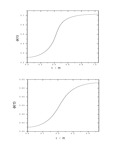
Figure 2: The instanton, $\phi(\tau)$, as a function of the Euclidean time $\tau$ is shown for Einstein GR and BW. The upper panel shows the case $\beta=10$, and the lower panel shows the case $\beta=10^{-3}$.

In Fig. 3 we show $|V^{{}^{\prime\prime}}|\,/\,H^{2}$ as a function of the Euclidean time $\tau$ for our models. From this plot we observe that most of the time during the tunneling we obtain $|V^{{}^{\prime\prime}}|\,>\,H^{2}$, analogous to that occurs in Einstein’s Theory of Relativity. Note that, for $\beta=10$, the peak becomes narrower and deeper, and thus the above inequality is better satisfied.

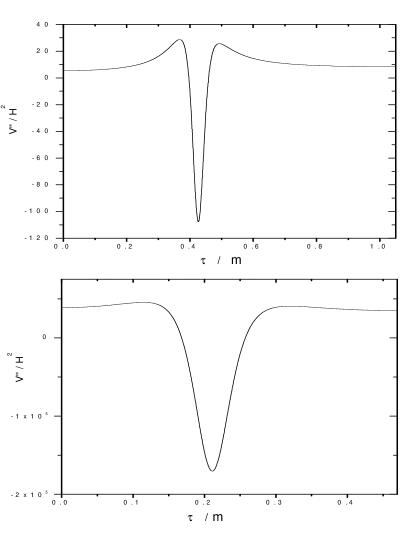
Figure 3: This plot shows how during the tunneling process the inequality $|V^{{}^{\prime\prime}}|\gg H^{2}$ holds. The GR lines represents the same inequality for Einstein’s Theory of Relativity. The upper panel shows this case, and the lower panel show the Gauss Bonnet Brane world case.

III Inflation after tunneling

After the tunneling has occurred, we make an analytical continuation to the Lorentzian space-time, and the time evolution of the scale factor $a(t)$ and the scalar field $\phi(t)$, are given by

$$\ddot{a} = a\beta_{q}m^{2\left(q-1\right)}\left(\frac{\dot{\phi}^{2}}{2}+V(\phi)\right)^{q}\left[1-\frac{3}{2}q\frac{\dot{\phi}^{2}}{\left(\frac{\dot{\phi}^{2}}{2}+V(\phi)\right)}\right],$$ (14)

$$\begin{array}[]{ll}&\ddot{\phi}+3\frac{\dot{a}}{a}\dot{\phi}+V_{,\phi}=0,\end{array}$$

respectively. Here the dots represent derivative with respect to cosmological time.

Before, to solve this equations we want to discuss the slow-roll approximation in order to justify in ours models the values of the parameters $\beta_{q}$’s and the mass of the inflaton field. During the inflationary epoch the energy density associated to the scalar field is of the order of the potential, i.e. $\rho\sim V$, where we have used the slow-roll conditions ($\dot{\phi}^{2}\ll V(\phi)$). Therefore, the Friedmann equation reduces to

$$H^{2}\approx\beta_{q}\,V^{q},$$ (15)

since we are interested in an inflationary universe model, the term proportional to $\frac{1}{a^{2}}$ is rapidly diluted. The field equation of motion for the field $\phi$ becomes

$$3H\dot{\phi}\approx-V_{,\,\phi}.$$ (16)

After the tunnel has occurred, the potential energy just corresponds to the chaotic scalar potential ($V(\phi)\simeq\,m^{2}\phi^{2}/2$) by integrating equation (16) in the slow roll approximation, we get for arbitrary $q$

$$\dot{\phi}(t)=-\frac{2^{q/2}\,m^{2-q}}{3\beta_{q}^{1/2}}\,\phi^{1-q},$$ (17)

and the full evolution of inflaton field in the Lorentzian era read as follows

$$\phi(t)=\left[\phi_{i}^{q}-\frac{2^{q/2}\,\,q\,m^{2-q}}{3\beta_{q}^{1/2}}\,t\right]^{1/q},$$ (18)

where $\phi_{i}$ is a constant and corresponds to the initial value of the scalar field $\phi$. On the other hand, the scale factor results to be

$$a(t)=a_{i}\,\exp\left(\frac{\beta_{q}^{1/2}\,m^{2}}{2^{q/2}}\,t\left[\phi_{i}^{q}-\frac{2^{q/2}\,\,q\,m^{2-q}}{6\beta_{q}^{1/2}}\,t\right]\right).$$ (19)

Where we can see that the energy density associated to the inflaton field decreases in order to reach the kinetic epoch ($\rho_{kin}\sim a^{-6}$) and the scale factor satisfies the condition $\ddot{a}>0$.

The consequences of the dynamics of an open inflationary universe, such as, slow roll parameters, density perturbations and tensor perturbations are quite complicate to be realized, since it involves several contributions. As was shown in Refs. re6 ; ramon ; delCampo:2004gh ; del Campo:2004ee in an open inflationary universe model this correction should be somewhat corrected during the very first stages of the inflationary period, at $N=O(1)$. For instance, during the first three e-folds the fluctuations of the inflaton field are not produced inside the bubble. In this way one may since $N$ should be of order hundred or more in order to solve the cosmological ”puzzles”, we may get rid of them and consider the standard flat-space expressions give correct results for $N>3$.

In order to constrain the parameters of our model we considered the dimensionless slow-roll parameters Kim:2004gs ; Kim:2004jc ; Kim:2004hu ; Murray:2006fw ,

$$\epsilon=-\frac{\dot{H}}{H^{2}}=\frac{q}{6\beta_{q}}\,\frac{V_{\,,\phi}^{2}}{V^{q+1}},\;\;\;\,\eta=\frac{V_{\,,\phi\phi}}{3H^{2}}=\frac{V_{\,,\phi\phi}}{3\beta_{q}\,V^{q}}.$$ (20)

The condition under which we could that ensure that the inflationary epoch could take place can be summarized with the inequality $\epsilon<1$ (note that this condition is analogue to the requirement that $\ddot{a}>0$). Inflation ends when the field takes the value,

$$\phi_{f}\simeq\left[\frac{2^{q+1}\,q\,m^{2(1-q)}}{6\beta_{q}}\right]^{1/2q},$$ (21)

or equivalently, in term of the value of potential at the end of inflation,

$$V_{f}\simeq\,\frac{q\,m^{2}}{3\,\beta_{q}}.$$ (22)

In the following, the subscripts $*$ and $f$ are used to denote the epoch when the cosmological scale exits the cosmological horizon and the end of inflation, respectively. At the end of inflation we can compute the number of e-folds which is given by

$$N=\int_{t_{*}}^{t_{f}}\,H\,dt^{\prime}=-3\int_{\phi_{*}}^{\phi_{f}}\frac{H^{2}}{V_{,\,\phi}}d\phi^{\prime}=-3\,\beta_{q}\int_{\phi_{*}}^{\phi_{f}}\frac{V^{q}}{V_{,\,\phi}}d\phi^{\prime},$$ (23)

and using the chaotic potential the number of e-folds becomes

$$N\simeq\,\frac{3\beta_{q}}{2q\,m^{2}}\,\left(\frac{m}{\sqrt{2}}\right)^{2q}\,[\phi_{*}^{2q}-\phi_{f}^{2q}]\simeq\frac{3\beta_{q}}{2q\,m^{2}}\,[V_{*}^{q}-V_{f}^{q}]\simeq\frac{3\beta_{q}}{2q\,m^{2}}\,V_{*}^{q}-\frac{1}{2}.$$ (24)

In order to study the scalar perturbations of the inflaton fields we considerer that the conservation of energy-momentum on the brane, ($\nabla^{\nu}T_{\nu\mu}=0$), implies that the adiabatic matter curvature perturbation $\zeta$ over one uniform density hypersurface is conserved on large scales, independent of the gravitational physics Wand . Consequently, the amplitudes of a given mode that re-enters the Hubble radius after inflation is given by

$$A_{S}^{2}\;|_{k=k_{*}=aH}=\,\left.\frac{H^{4}}{2\pi^{2}\dot{\phi}^{2}}\right|_{k_{*}=aH}=\left.\frac{9}{2\pi^{2}}\,\frac{H^{6}}{V_{\,,\phi}^{2}}\right|_{k_{*}=aH}=\left.\frac{9\,\beta_{q}^{3}}{2\pi^{2}}\,\frac{V^{3q}}{V_{\,,\phi}^{2}}\right|_{k_{*}=aH}=\frac{9\,\beta_{q}^{3}}{4\pi^{2}}\,\frac{V_{*}^{3q-1}}{m^{2}}.$$ (25)

Finally, from Eqs.(24) and (25) we obtain a constrain on the ratio

$$\frac{m^{2/q-4}}{\beta_{q}^{1/q}}=\frac{9}{4\pi^{2}}\,\frac{1}{A_{s}^{2}}\,\left[\frac{q\,(2\,N+1)}{3}\right]^{\frac{3q-1}{q}}.$$ (26)

This latter expression allows us to fix the values of the parameters of our model. The needed $N\sim 65$ e-folds of inflations after tunneling has occurred, in order to solve of the most cosmological puzzles. On the other hand, $A_{S}\sim 10^{-5}$ in order to fit over the observational data.

Finally, we solve the Lorentzian field Equations (14) numerically, we use the following boundary conditions: $\dot{\phi}(0)=0$, $a(0)=0$ and $\dot{a}(0)=1$. As in re6 ,shiba and ramon , the scalar field slowly rolls down to its minimum of the effective potential, and its field starts to oscillate near the minimum. During this stage, the $N$ e-folds parameter presents different values for our models. The results are summarized in Figure 4.

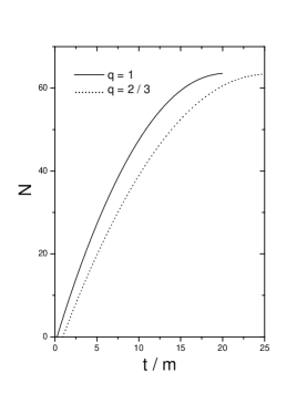
Figure 4: The plot shows the number $N$ of e-folds as a function of the scaled cosmological times $t/m$. The solid line represents Einstein’s Theory of Relativity, and the dashed line represents the Gauss Bonnet Brane World.

IV conclusion

In this paper we have studied one-field open inflationary universe models in which the gravitational effects are described by Gauss-Bonnet Brane World cosmology. In this kind of theory, the Friedmann equation have a complicated structure as show by Eq. (3) and at the limits of Gauss-Bonnet and 4D regime we obtain an effective Friedmann equation whose form is given by term: $\beta_{q}\rho^{q}$, where $q=2/3$ and $q=1$ for the GB and 4D Einstein’s Theory of Relativity respectively. We have described solutions for the Euclidean fields Eqs.(11) with an effective potentials describe in Ref.re6 in which the CDL instanton exist. The existence of this instanton becomes guaranteed since the inequality $|V^{{}^{\prime\prime}}|>H^{2}$ is satisfied, and in the case of $q=2/3$ this inequality is most stronger satisfy ($|V^{{}^{\prime\prime}}|\gg H^{2}$) than the Einstein-Hilbert case ($q=1$). Therefore, the conditions for create an open inflationary universes are better satisfied in the context of Gauss-Bonnet Brane world cosmology, and thus, with the slow-roll approximation, inflationary universes models are realized. For the two values i.e.($q=1$ and $q=2/3$), $V^{{}^{\prime\prime}}$ remains greater than $H^{2}$ during the first e-folds of inflation.

We also found that the modification of the Friedmann equation ($\rho^{q}$) improves the characteristics of inflation . This is accentuated in the number of the e-folds $N$ if we take a little different values for $\beta_{2/3}$ parameter as it is shown by Eq.(24).

For $m\sim 10^{-6}$ we have found that, the scalar potential ($V_{f}$) at the end of inflationary epoch in the Gauss Bonnet Brane cosmology ($q=2/3$) is greater than the standard general relativity ($q=1$). In theory with Gauss Bonnet correction the ”velocity” ($\dot{\phi}$) of scalar field decreased in comparison with the theory without correction term. This remark it is explicitly show by Eq.(17). Consequently, in the Gauss Bonnet brane world cosmology the time interval required to generate the appropriate N e-folds numbers of inflations, in order to solve of the most cosmological puzzles, becomes greater than in comparison with the general relativity theory ($q=1$). This is shown in figure 4. Eq. (26) shows the possible constraint between the mass parameter of the inflaton field $m$ and the parameter $\beta_{q}$. This constraint is quite strong related to observational data through the N e-folds number and the amplitude of the scalar perturbation ($A_{S}$). It is well know that, when $q=1$ the parameter $\beta_{1}$ is fixed ($\beta_{1}=\frac{8\pi}{3}\sim O(10)$), then from Eq.(26) we can establish the mass parameter of the inflaton field by $m\sim 10^{-6}$, which corresponds to its standard value. When $q=2/3$ the parameter $\beta_{2/3}$ is given by the value of the Gauss Bonnet coupling constant ($\beta_{2/3}=\beta_{2/3}(\alpha)\sim 1/\alpha$). If we consider the fact that $\alpha\sim 1/g_{s}$ where $g_{s}$ is the scale of the string theory, the value obtained from Eq.(26) for the mass parameter is extremely large. Finally, from Eq. (26) we can change both parameters in order to fit ours results with observational data. This changing the constraint of the parameter $\beta_{2/3}$, and we would also change the value of the Gauss-Bonnet coupling constant ($\alpha$) arise from string theory. For example, if we consider the well know value for the mass of the inflaton field ($m\sim 10^{-6}$), we obtain that $\beta_{2/3}\sim 10^{-3}$.

- (1) C.L. Bennett et al.Astrophys. J. Suppl. 148, 1 (2003).
- (2) J. P. Uzan, U. Kirchner and G. F. R. Ellis, Mon.Not.Roy.Astron.Soc.L 65, 344 (2003).
- (3) B. Ratra and P. J. E. Peebles, Astrophys. J. Lett. 432, L5 (1994);
- (4) B. Ratra and P. J. E. Peebles, Phys. Rev. D 52, 1837 (1995).
- (5) A. Linde, Phys. Rev. D 59 , 023503 (1998).
- (6) A. Linde, M. Sasaki and T. Tanaka, Phys. Rev. D 59, 123522 (1999).
- (7) T. Chiba and M. Yamaguchi, Phys.Rev.D 61, 027304 (2000).
- (8) S. del Campo and R. Herrera, Phys.Rev.D 67, 063507 (2003).
- (9) S. del Campo, R. Herrera and J. Saavedra, Phys. Rev. D 70, 023507 (2004).
- (10) S. del Campo, R. Herrera and J. Saavedra, Int. J. Mod. Phys. D 14, 861 (2005).
- (11) L. Balart, S. del Campo, R. Herrera, P. Labrana and J. Saavedra, Phys. Lett. B 647, 313 (2007).
- (12) M. Bouchmadi and P. F. González-Días, Phys. Rev. D 65, 063510 (2002).
- (13) M. Bouchmadi and P. F. González-Días and A. Zhuk Class.Quant.Grav. 19 , 4863 (2002).
- (14) G. Kofinas, R. Maartens, E. Papantonopoulos. hep-th/0307138.
- (15) P. Horava and E. Witten, Nucl.Phys.B 475, 94 (1996).
- (16) P. Horava and E. Witten, Nucl.Phys.B 460, 506 (1996) .
- (17) J. Lidsey, astro-ph/0305528.
- (18) P. Brax, C. van de Bruck. Class.Quant.Grav.20, R201-R232 (2003).
- (19) E. Papantonopoulos, Lect.Notes Phys. 592, 458 (2002).
- (20) R. Maartens, D. Wands, B. A. Bassett, I. Heard, Phys.Rev.D 62, 041301 (2000).
- (21) X. H. Meng and P. Wang, Class. Quant. Grav. 21, 2527 (2004)
- (22) J. E. Lidsey and N. J. Nunes, Phys. Rev. D 67, 103510 (2003)
- (23) G. Calcagni and S. Tsujikawa, Phys. Rev. D 70, 103514 (2004).
- (24) H. Kim, K. H. Kim, H. W. Lee and Y. S. Myung, Phys. Lett. B 608, 1 (2005).
- (25) K. H. Kim and Y. S. Myung, JCAP 0412, 004 (2004).
- (26) K. H. Kim and Y. S. Myung, Int. J. Mod. Phys. D 14, 1813 (2005).
- (27) B. M. Murray and Y. S. Myung, Phys. Lett. B 642, 426 (2006).
- (28) B. M. Leith and I. P. Neupane, JCAP 0705, 019 (2007).
- (29) T. Koivisto and D. F. Mota, Phys. Rev. D 75, 023518 (2007).
- (30) A. K. Sanyal, Phys. Lett. B 645, 1 (2007).
- (31) T. Koivisto and D. F. Mota, Phys. Lett. B 644, 104 (2007).
- (32) B. M. N. Carter and I. P. Neupane, JCAP 0606, 004 (2006).
- (33) S. Nojiri, S. D. Odintsov and O. G. Gorbunova, J. Phys. A 39, 6627 (2006).
- (34) S. Nojiri, S. D. Odintsov and M. Sasaki, Phys. Rev. D 71, 123509 (2005).
- (35) S.C. Davis, Phys. Rev. D67 (2003) 024030.
- (36) D. Wands et. al., Phys. Rev. D 62, 043527 (2000).