Two-Dimensional Electron Gas with Cold Atoms in Non-Abelian Gauge Potentials

Abstract

Motivated by the possibility of creating non-Abelian fields using cold atoms in optical lattices, we explore the richness and complexity of non-interacting two-dimensional electron gases (2DEGs) in a lattice, subjected to such fields. In the continuum limit, a non-Abelian system characterized by a two-component “magnetic flux” describes a harmonic oscillator existing in two different charge states (mimicking a particle-hole pair) where the coupling between the states is determined by the non-Abelian parameter, namely the difference between the two components of the “magnetic flux”. A key feature of the non-Abelian system is a splitting of the Landau energy levels, which broaden into bands, as the spectrum depends explicitly on the transverse momentum. These Landau bands result in a coarse-grained “moth”, a continuum version of the generalized Hofstadter butterfly. Furthermore, the bands overlap, leading to effective relativistic effects. Importantly, similar features also characterize the corresponding two-dimensional lattice problem when at least one of the components of the magnetic flux is an irrational number. The lattice system with two competing “magnetic fluxes” penetrating the unit cell provides a rich environment in which to study localization phenomena. Some unique aspects of the transport properties of the non-Abelian system are the possibility of inducing localization by varying the quasimomentum, and the absence of localization of certain zero-energy states exhibiting a linear energy-momentum relation. Furthermore, non-Abelian systems provide an interesting localization scenario where the localization transition is accompanied by a transition from relativistic to non-relativistic theory.

I Introduction

Methods for creating fields that couple to neutral atoms in the same way that electromagnetic fields couple to charged particles have created the exciting possibility of studying the effects of a generalized magnetism using cold atoms.mono ; NJP ; NA Using laser induced hopping, a controlled phase can be imposed upon particles moving along a closed loop in an optical lattice. The associated synthetic fields can be sufficiently strong to enter the regime of exotic magnetic phenomena that have been difficult to explore in condensed matter experiments, such as the fragmented fractal spectrum of a two dimensional electron gas (2DEG) in a magnetic field, the famous “Hofstadter butterfly”Hofs . Such fields need not obey Maxwell’s equations, thus providing the possibility of discovering fundamentally new physics. Escher . For example, we discuss here the generation of non-Abelian fields, by using cold atoms that occupy two Zeeman states in the hyperfine ground level NA ; these two states may be thought of as “colors” of the gauge fields, and such a system may be used to simulate lattice gauge theories in (2+1) dimensions. Other potential applications of non-Abelian fields are the creation of counterparts of magnetic monopoles mono , and integer and fractional quantum Hall effects.chern

In this paper, we adopt the 2DEG as a motif for the study of cold atom systems. The subject of 2DEGs in a magnetic field is a textbook topic Prange , as the problem maps to a one-dimensional harmonic oscillator. The discrete energy levels of the oscillator are the Landau levels that describe free particle energies in terms of the quantized units $\hbar\omega_{c}$, where $\omega_{c}=eB/mc$ is the cyclotron frequency of the corresponding classical motion. Each level is highly degenerate, reflecting the fact that a classical electron spirals about a line parallel to the magnetic field, with an arbitrary center in the transverse plane. The degree of degeneracy is equal to $L^{2}/2\pi\delta^{2}$ where $\delta=\sqrt{\hbar c/eB}$ is the magnetic length and $L^{2}$ is the area of the system.

Beginning with the celebrated work of Onsager Ons , Harper Harper and then Hofstadter Hofs , the subject of 2DEGs in a crystalline lattice in a magnetic field has fascinated physicists as well as mathematicians. In the presence of a lattice, each Landau energy level splits into $Q$ bands, where the rational number $P/Q$ is the magnetic flux through the unit cell in units of the magnetic flux quantum (fluxoid). The heart of the problem is the two competing periodicities related to the ratio of the reciprocal of the cyclotron frequency and the period of the motion of the electron in the periodic lattice. Two key aspects that have been explored extensively are the exotic multifractal spectrum (Hofstadter butterfly), and the metal-insulator transition obtained by tuning the ratio of the tunneling along the two directions of the lattice Harper . Recent studies have shown that these properties can be demonstrated using ultracold atoms in an artificial magnetic field  NJP ; Drese . This paper revisits the metal-insulator transition when the 2DEG is subjected to a non-Abelian gauge field which is a natural generalization of the uniform magnetic field. Such fields yield a much richer spectral and transport landscape than is encountered in the Abelian case.

The generic experimental setup for producing non-Abelian $U(2)$ gauge fields that we consider here, consists of a two-dimensional optical lattice populated with cold atoms that occupy two hyperfine states NJP ; NA . Such systems exhibit three competing length scales , associated with two distinct “magnetic fluxes” (denoted by $\alpha_{1}$ and $\alpha_{2}$) that penetrate the unit cell. Our aim is to describe some of the generic properties of such systems. Although our main focus is on optical lattices, we first discuss the corresponding continuum problem, where the the infinite degeneracy of the Landau levels is lifted by non-Abelian interactions. The continuum problem mirrors some of the features subsequently encountered in the lattice system.

In the discussion of the metal-insulator transition in the lattice, we focus on the ground state as well as the states at the band center. These two cases are respectively relevant for experimental systems involving Bose condensates and fermionic gases near half-filling. Some of these results were described in an earlier paper prl . In addition to a detailed analysis, here we describe new results, such as the simulation of relativistic phenomena using cold atoms in non-Abelian fields. By tuning lattice anisotropy, we can implement relativistic as well as non-relativistic dynamics, with a particular focus on the effects of disorder. Simulation and detection of Dirac fermions using single-component cold atoms in a hexagonal lattice was recently proposed duan . The systems we propose here provide the possibility of observing relativistic particles and also of studying their localization properties. We show that the non-Abelian systems provide an experimental realization of the defiance of localization by disordered relativistic fermions, a topic that has been the subject of extensive study Fradkin .

In Section II, we introduce non-Abelian gauge fields and the corresponding effective “magnetic fields.” Section III examines the continuum limit of a single particle in a non-Abelian gauge field. In Section IV, we discuss lattice systems subjected to these fields, and describe methods of calculation. In Section V, we study various spectral characteristics of the non-Abelian lattice systems. There, following long establised practice for studying metal-insulator transition in Abelian systems, we fix $\alpha_{1}=(\sqrt{5}-1)/2$, the golden mean, which we denote as $\gamma$. The irrationality of $\alpha_{1}$ ensures the existence of a localization transition.Harper ; Sok For $\alpha_{2}$, we consider a selected set of both rational and irrational values. Sections VI and VII discuss localization properties of the states at the band center ($E=0$) and at the band edge. The localization of the $E=0$ states brings out some of the most important features of the non-Abelian cases, including the dependence of the transition upon a conserved momentum. Furthermore, a unique aspect of the the non-Abelian system, namely the defiance of localization of the $E=0$ states, emerges when the energy-momentum relation mimics the behavior of relativistic particles. Section VIII describes the experimental realization of the metal-insulator transition in cold atom lattices.

II Non-Abelian Gauge Fields

Effective non-Abelian vector potentials arise naturally in systems where the atoms have $N$ degenerate internal states. The most general vector potential couples the states, and thus gives rise to a $U(N)$ gauge symmetry. We here consider the case where $N=2$. In our treatment of the non-Abelian case, we follow the convention of an earlier study NA , adopting its form of vector potential,

$$\vec{A} = \frac{\hbar c}{ea}\left(\frac{\pi}{2}\left(\begin{array}[]{cc}-1&1\\ 1&-1\\ \end{array}\right),\>2\pi\frac{x}{a}\left(\begin{array}[]{cc}\alpha_{1}&0\\ 0&\alpha_{2}\\ \end{array}\right),\>0\right).$$ (5)

The $\alpha_{i}$ determine the “magnetic fluxes” of the lattice with lattice constant $a$.

Equation (5) is in the Landau gauge: $\vec{A}(x,y)=(A_{x},A_{y}(x),0)$, where $A_{x}$ is a constant and $A_{y}$ depends only on $x$.

We rewrite the vector potential in terms of Pauli matrices $\sigma_{i}$, separating the Abelian and the non-Abelian parts of the gauge field,

$$\vec{A} = \frac{\hbar c}{ea}\left[-\frac{\pi}{2}(I-\sigma_{x})\hat{\mathbf{x}}+2\pi\frac{x}{a}\alpha I\hat{\mathbf{y}}+\Delta\,\frac{x}{a}\sigma_{z}\hat{\mathbf{y}}\right],$$ (6)

where we have defined quantities $\alpha=(\alpha_{1}+\alpha_{2})/2$ and $\Delta=\pi(\alpha_{1}-\alpha_{2})$. Here $\sigma_{a}$, $a=x,y,z$ denotes Pauli matrices. The parameter $\Delta$ characterizes the non-Abelian feature of the system.

For non-Abelian fields, the effective “magnetic field” is given by,

$$\hat{\mathbf{B}}=\nabla\times\hat{\mathbf{A}}-\frac{ie}{\hbar c}\hat{\mathbf{A}}\times\hat{\mathbf{A}}.$$ (7)

The origin of the extra term $\hat{\mathbf{A}}\times\hat{\mathbf{A}}$ can be traced to the commutator for the generalized velocity operator $(p-\frac{e}{c}A)/M$,

$$[v_{n},v_{m}] = \frac{\hbar e}{M^{2}c}\left(\partial_{n}A_{m}-\partial_{m}A_{n}-\frac{ie}{\hbar c}[A_{n},A_{m}]\right)$$

$$= \frac{i\hbar e}{M^{2}c}\epsilon_{mnr}B_{r}.$$

For the vector potential in Eq. (5), this gives

$$\hat{B}_{z}=\hat{B}_{0}+\Delta\left(\frac{\hbar c}{ea^{2}}\right)(\hat{\mathbf{\sigma}}_{z}-\pi\frac{x}{a}\hat{\mathbf{\sigma}}_{y}),$$ (8)

where $B_{0}=2\pi\alpha(\frac{\hbar c}{ea^{2}})$. Thus, $\alpha=B_{0}a^{2}/(2\pi\hbar c/e)$ describes the Abelian flux quanta penetrating per unit cell of the lattice. The non-Abelian gauge potential generates a non-uniform magnetic field, as $\hat{\mathbf{B}}$ depends explicitly on the spatial coordinate $x$ when $\Delta\neq 0$.

III Continuum Limit of the Non-Abelian System

We now consider the continuum limit of the non-Abelian problem. Although the $\hat{\mathbf{A}}$ of the Eq. (6) is ill-defined in the continuum limit $a\rightarrow 0$, the study is useful in illustrating some key aspects of the non-Abelian systems. In general, continuum problems can also be experimentally realized, as in Ref. mono .

It can be shown, after some algebra, that the two-component continuum Hamiltonian $\hat{\mathbf{H}}_{c}=(\hat{\mathbf{p}}-\frac{e}{c}\hat{\mathbf{A}})^{2}/(2M)$ resulting from the vector potential in Eq. (6) is gauge-equivalent to

$$\hat{\mathbf{H}} = \frac{1}{2M}\left(\begin{array}[]{cc}(\hat{p}_{x}+\beta)^{2}+V(x)&C\Delta(x-x_{0})^{2}\\ C\Delta(x-x_{0})^{2}&(\hat{p}_{x}-\beta)^{2}+V(x)\end{array}\right)$$ (11)

up to a $k_{y}$ dependent term. The transverse momentum $k_{y}$ is a conserved quantity as the Hamiltonian $\hat{\mathbf{H}}_{c}$ with $\vec{A}$ given by Eq  6 is cyclic in $y$. Here, $\beta=\frac{\hbar\pi}{2a}$, $C=8\pi^{2}\alpha(\beta/a)^{2}$ ,$V(x)=M^{2}\omega^{2}x^{2}/2$ with $\omega=\frac{2\pi\beta}{ma}\sqrt{(\alpha_{1}^{2}+\alpha_{2}^{2})/2}$ and $x_{0}=2\pi a\frac{\hbar k_{y}\beta}{M^{2}\omega^{2}a}\frac{\alpha_{1}\alpha_{2}}{\alpha}$. This particular form of the Hamiltonian provides a new, illuminating picture of the non-Abelian problem; the particle behaves as a two-component harmonic oscillator existing in a positive as well as a negative charge state. The physics of this system is that of a particle-hole pair, with the non-Abelian parameter $\Delta$ , governing the coupling between states.

The spectrum of $\hat{\mathbf{H}}_{c}$ is obtained by numerical diagonalization in a basis of harmonic oscillator wave functions with frequency $\omega$. Figure (1) shows the six lowest energy levels. For fixed $k_{y}$, at $\Delta=0$, each Landau level is two-fold degenerate. For $\Delta\neq 0$ the degeneracy is lifted and the eigenstates become entangled states of a particle-hole pair.

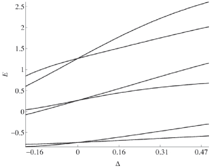
Figure 1: Six lowest energy levels of the continuum non-Abelian Hamiltonian in Eq. (11), $\beta=\pi/2,M=1,k_{y}=1$ and $2\pi\alpha_{1}=1$. The levels are equally spaced in (and only in) the Abelian case, $\Delta=0$, where the system reduces to two decoupled harmonic oscillators.

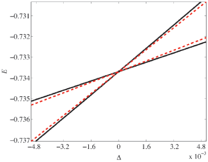
Figure 2: (color online) The ground state splitting obtained numerically (see Fig. 1) (solid black), compared with that obtained by perturbation theory (dashed red) about the Abelian point $\Delta=0$.

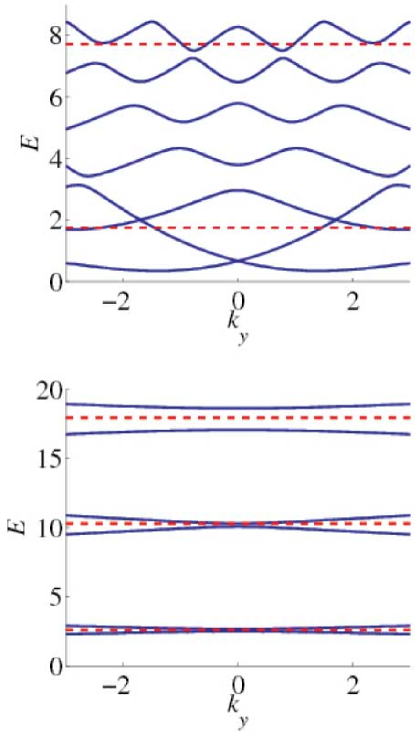
Figure 3: (color online) The three lowest energy levels of the non-Abelian system with $\alpha_{1}=1.32$ and $\alpha_{2}=0.253$ (top), $\alpha_{2}=1.11$ (bottom). The dashed line shows the Abelian levels corresponding to $\sqrt{\frac{1}{2}(\alpha_{1}^{2}+\alpha_{2}^{2})}$.

As Fig. 1 shows, the energy levels are equally spaced only for the Abelian case, $\alpha_{1}=\alpha_{2}$. We can explicitly understand the splitting of each Landau level via degenerate perturbation theory, with $\Delta$ as a small parameter and using degenerate eigenstates,

$$f_{1}^{n}=e^{ik_{y}y}\left(\begin{array}[]{cc}e^{-i\beta x}\psi_{n}(x)\\ 0\end{array}\right),\>f_{2}^{n}=e^{ik_{y}y}\left(\begin{array}[]{cc}0\\ e^{i\beta x}\psi_{n}(x)\end{array}\right),$$

where $\psi_{n}(x)$ are the eigenstates of the corresponding harmonic oscillator. Figure 2 compares the perturbative splitting of the lowest Landau level with the numerical result.

Figure 3 shows the variation of the energies with $k_{y}$, obtained numerically. In highly non-Abelian cases, the energies bear no relation to their Abelian values. Close to the Abelian limit (bottom) the energy levels are simply split around the Abelian energies. The energies oscillate with $k_{y}$, resulting in actual and avoided crossings (i.e., the Landau bands overlap). In the vicinity of the crossings, the bands exhibit a linear dispersion relation. As we shall discuss, these features reappear in the corresponding problem of the non-Abelian gauge field on an optical lattice.

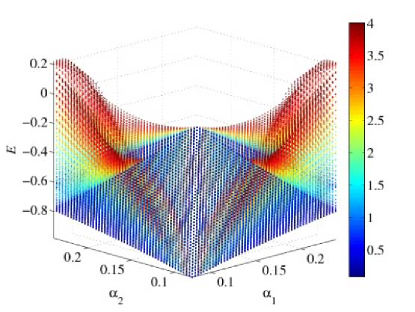
Figure 4: (color online) The continuum version of the Hofstadter “moth” NA . This plot shows the energies as a function of $\alpha_{1}$ and $\alpha_{2}$ for a range of $k_{y}$; the color scale indicates the range of $k_{y}$. Along the line $\alpha_{1}=\alpha_{2}$ , the Abelian “backbone” of the moth, there is no $k_{y}$ dependence.

Figure 4 summarizes the effects of the non-Abelian gauge potential on the lowest Landau level of the corresponding Abelian problem. The figure describes the continuum limit of the Hofstadter “moth” NA , which is the generalization of the Hofstadter “butterfly” as the underlying gauge field becomes non-Abelian. This coarse-grained “moth” illustrates the symmetry breaking feature of the non-Abelian system as it lifts the degeneracy of the corresponding Abelian problem.

IV Two-Dimensional Lattice in Non-Abelian Gauge Fields

Our starting point is a tight binding model (TBM) of a particle moving on a two-dimensional rectangular lattice $(x,y)$, with lattice constants $(a,b)$ and nearest-neighbor hopping characterized by the tunneling amplitudes $(J,J\Lambda)$. When a weak external vector potential, $\vec{A}(x,y)=(A_{x},A_{y},0)$, is applied to the system, the Hamiltonian,

$$\hat{H}=-J\left[\cos\left((p_{x}-\frac{e}{c}A_{x})\frac{a}{\hbar}\right)+\Lambda\cos\left((p_{y}-\frac{e}{c}A_{y})\frac{b}{\hbar}\right)\right],$$

where $\vec{p}$ is the momentum operator. Alternatively, the Hamilonian of a 2DEG on a lattice in the presence of a magnetic fied can be written as,

$$H=-\sum_{<ij>}J_{ij}c_{j}^{\dagger}c_{i}e^{i\theta_{ij}}+H.C.$$ (13)

where $c_{i}$ is the usual fermion operator at site $i$. The $J_{ij}$ is the nearest-neighbor anisotropic hopping with values $J$ and $J\Lambda$ along the $x$ and the $y$-direction.

The phase factor $\theta_{ij}=-\theta_{ji}$ defined on a link $<i,j>$ is identified as $(2\pi e/ch)\oint{\bf A}.{\bf dl}$, where ${\bf A}$ is the vector potential, and

$$frac{1}{2\pi}\sum_{unit{}cell}\theta_{ij}=e/ch\oint{\bf A}.{\bf dl}=\frac{1}{\Phi_{0}}\oint{\bf B}.{\bf dS}$$ (14)

is the magnetic flux penetrating the unit cell in units of magnetic flux quantum, $\Phi_{0}=ch/e$.

We denote the eigenfunction (projected onto the $x,y$ basis), corresponding to the eigenvalue equation $H|\Psi>=E|\psi>$ as $\Psi(x,y)$. With the transverse wave number of the plane wave as $\tilde{k}_{y}=k_{y}/a$, the wave function can be written as: $\Psi(ma,na)=e^{i2\pi k_{y}n}{\bf g}_{m}$ with $x=ma$ and $y=na$.

Subsituting the vector potential defined in the Eq.  6, the two-component vector ${\bf g}_{m}=\left(\begin{array}[]{cc}\theta_{m}\\ \eta_{m}\end{array}\right)$ can be shown to result in the following equations,

$$\left(\begin{array}[]{cc}\theta_{m+1}\\ \eta_{m+1}\end{array}\right)+\left(\begin{array}[]{cc}\theta_{m-1}\\ \eta_{m-1}\end{array}\right)-\left(\begin{array}[]{cc}0&E-V_{m}\\ E-U_{m}&0\end{array}\right)\left(\begin{array}[]{cc}\theta_{m}\\ \eta_{m}\end{array}\right)=0,$$

where

$$U_{m} = 2\Lambda\cos(2\pi\alpha_{1}m-2\pi k_{y}),$$

$$V_{m} = 2\Lambda\cos(2\pi\alpha_{2}m-2\pi k_{y}).$$

For $\alpha_{1}=\alpha_{2}$ (mod 1), we recover the Abelian limit described by the Harper equation Harper

$$g_{m+1}+g_{m-1}+2\Lambda\cos(2\pi\alpha m-2\pi k_{y})g_{m}=E\,g_{m},$$ (16)

For irrational values of the flux $\alpha$, the system exhibits a metal-insulator transition at $\Lambda=1$.

The approach to the irrational values of $\alpha_{i}$ is studied by considering a sequence of periodic systems obtained by rational approximants $\alpha_{i}=p_{i}/q_{i}$. This corresponds to truncating the continued fractional expansion of $\alpha_{1}$ and $\alpha_{2}$. The resulting periodic system will have period $Q$, the least common multiple of $q_{1}$ and $q_{2}$.

The $2Q$-dimensional system can be cast in the form of two $Q$-dimensional eigenvalue problems:

$$\left(\begin{array}[]{cccccccc}U_{1}&1&0&0&.&.&.&e^{-ik_{A}}\\ 1&V_{2}&1&0&0&.&.&0\\ 0&1&U_{3}&1&0&.&.&0\\ 0&0&1&V_{4}&1&0&.&0\\ 0&0&0&1&U_{5}&1&.&0\\ .&.&.&.&.&.&.&.\\ e^{ik_{A}}&.&.&0&0&0&1&V_{Q}\end{array}\right)\>\left(\begin{array}[]{cc}\theta_{1}\\ \eta_{2}\\ \theta_{3}\\ \eta_{4}\\ .\\ .\\ .\\ \eta_{Q}\\ \end{array}\right)\>=E_{A}\left(\begin{array}[]{cc}\theta_{1}\\ \eta_{2}\\ \theta_{3}\\ \eta_{4}\\ .\\ .\\ .\\ \eta_{Q}\end{array}\right)\>$$

and

$$\left(\begin{array}[]{cccccccc}U_{2}&1&0&0&.&.&.&e^{-ik_{B}}\\ 1&V_{3}&1&0&0&.&.&0\\ 0&1&U_{4}&1&0&.&.&0\\ 0&0&1&V_{5}&1&0&.&0\\ 0&0&0&1&U_{6}&1&.&0\\ .&.&.&.&.&.&.&.\\ e^{ik_{B}}&.&.&0&0&0&1&V_{1}\end{array}\right)\>\left(\begin{array}[]{cc}\theta_{2}\\ \eta_{3}\\ \theta_{4}\\ \eta_{5}\\ .\\ .\\ .\\ \eta_{1}\\ \end{array}\right)\>=E_{B}\left(\begin{array}[]{cc}\theta_{2}\\ \eta_{3}\\ \theta_{4}\\ \eta_{5}\\ .\\ .\\ .\\ \eta_{1}\end{array}\right)\>$$

Here $E_{A}$ and $E_{B}$ denote the two sets of eigenvalues of the two uncoupled systems. The allowed eigenenergies of the full system are the union of these two sets.

In the above two eigenvalue equations, we have used the Bloch condition,

$$\left(\begin{array}[]{cc}\theta_{2m-1+Q}\\ \eta_{2m+Q}\end{array}\right)\> = e^{ik_{A}Q}\left(\begin{array}[]{cc}\theta_{2m-1}\\ \eta_{2m}\end{array}\right),$$

$$\left(\begin{array}[]{cc}\theta_{2m+Q}\\ \eta_{2m+1+Q}\end{array}\right)\> = e^{ik_{B}Q}\left(\begin{array}[]{cc}\theta_{2m}\\ \eta_{2m+1}\end{array}\right).$$

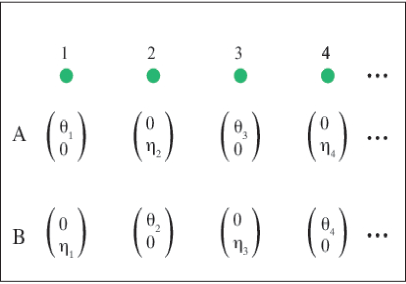
Figure 5: (color online) The two possible antiferrimagnetic states designated as A and B.

An important consequence of this decoupling of the $2Q$-dimensional problem into two $Q$-dimensional problems is that the eigenstates of the system are of an “antiferrimagnetic” type, as shown schematically in Fig. 5. We will refer to them as of the A and B-type. The corresponding states denoted as $\chi_{A}$ and $\chi_{B}$ are in general non-degenerate.

It is instructive to compare the eigenvalue formulation to the transfer matrix approach discussed in earlier studies NA . The TBM equation can be written as a transfer matrix equation,

$$\left(\begin{array}[]{cc}\theta_{m+1}\\ \eta_{m+1}\\ \theta_{m}\\ \eta_{m}\end{array}\right)\>=T(m)\left(\begin{array}[]{cc}\theta_{m}\\ \eta_{m}\\ \theta_{m-1}\\ \eta_{m-1}\end{array}\right),$$

where

$$T(m)=\left(\begin{array}[]{cccc}0&(E-V_{m})&-1&0\\ (E-U_{m})&0&0&-1\\ 1&0&0&0\\ 0&1&0&0\end{array}\right).$$

The allowed energies are those for which the product of $Q$ successive matrices $B(m)$ has an eigenvalue on the unit circle. $e^{\pm i\phi_{1}}$ and $e^{\pm i\phi_{2}}$. Alternatively, the 4-dimensional transfer matrix equation can be reduced to two independent 2-dimensional transfer matrices as

$$\left(\begin{array}[]{cc}\theta_{m+2}\\ \eta_{m+1}\\ \end{array}\right)\> = T_{A}(m)\left(\begin{array}[]{cc}\theta_{m}\\ \eta_{m-1}\\ \end{array}\right),$$ (27)

$$\left(\begin{array}[]{cc}\theta_{m+1}\\ \eta_{m}\\ \end{array}\right)\> = T_{B}(m)\left(\begin{array}[]{cc}\theta_{m-1}\\ \eta_{m-1}\\ \end{array}\right),$$ (32)

where the 2x2 matrices $T_{A}$ and $T_{B}$ are given by,

$$T_{A}(m)=\left(\begin{array}[]{cc}(E-V_{m+1})(E-U_{m-1})-1&-(E-V_{m+1})\\ (E-U_{m})&-1\\ \end{array}\right)\>$$

and

$$T_{B}(m)=\left(\begin{array}[]{cc}(E-V_{m})(E-U_{m-2})-1&-(E-U_{m})\\ (E-V_{m-1})&-1\\ \end{array}\right).\>$$

This decoupling of the $4$-dimensional transfer matrix problem into two $2$-dimensional transfer matrices is equivalent to the decoupling discussed earlier for the eigenvalue problem, which in turn implies the possibility of “antiferrimagnetic” type states as shown in Fig. 5. An important consequence of this type of state is that (out of four), only two of the eigenvalues of the $4$-dimensional transfer matrix have to be on the unit circle. In other words, in contrast to the statement made in an earlier paper NA , the allowed energies include states where two of the four eigenvalues of the transfer matrix are not on the unit circle prl .

The existence of “antiferrimagnetic” states and the relationship between the direct diagonalization method and the transfer matrix approach can be illustrated by considering a simple non-Abelian system, namely the one with $\alpha_{1}=1/2$ and $\alpha_{2}=0$ which can be treated analytically.

Diagonalization of two independent 2x2 matrices Eq. (32) gives

$$E_{A}(k_{A},k_{y}) = 2\left[\Lambda\cos 2\pi k_{y}\pm\cos k_{A}\right],$$

$$E_{B}(k_{B},k_{y}) = \pm 2\sqrt{\Lambda^{2}\cos^{2}2\pi k_{y}+\cos^{2}k_{B}},$$

and the corresponding eigenvectors

$$\chi_{A}=\left(\begin{array}[]{cc}\pm e^{-ik_{A}}\\ 0\\ 1\\ 0\end{array}\right),\>\chi_{B}=\left(\begin{array}[]{cc}0\\ e^{-ik_{B}}\frac{E/2\pm\Lambda\cos 2\pi k_{y}}{\cos k_{B}}\\ 0\\ 1\end{array}\right).$$

In general, the A and the B-states are non-degenerate. As is explicit in this example, the magnitude of the two components of the vectors are in general unequal, and hence the solutions correspond to antiferrimagnetic states. However, at $k_{y}=\pi/2$, the $E_{A}=E_{B}$ and the two degenerate states are antiferrimagnetic.

The spectrum can also be obtained by iterating the transfer matrix problem where the energies can be written in terms of the eigenvalues of the transfer matrix, $e^{\pm i\phi_{A}},e^{\pm i\phi_{B}}$. Comparison of the spectrum obtained by these two methods shows that $\phi_{A}=k_{A}/2$ and $\phi_{B}=k_{B}/2$.

The results of this paper were obtained using the direct diagonalzation method. We shall henceforth set $\alpha_{1}=\gamma$, the golden mean, and explore various complexities of the problem for different values of $\alpha_{2}$.

V Non-Abelian Spectrum for Irrational $\alpha_{1}$

The energy spectrum of the system is the union over $k_{y}$ of the individual energy spectra of the A and the B types of the tight binding equations. In the Abelian case, $\alpha_{1}=\alpha_{2}$, and when $\alpha_{1}$ is rational, equal to $p/q$, the spectrum consists of $q$ bands which are usually separated by gaps. As $k_{y}$ varies, the bands shift and their width may change, but they do not overlap, except at the band edges. For irrational $\alpha$, the spectrum is independent of $k_{y}$.

A striking aspect of the non-Abelian problem is the overlapping of the bands, as illustrated in figures 6 and  7. These figures depict two different classes of typical non-Abelian spectra with rational $\alpha_{2}$: In Fig.  6, type A and B solutions result in a non-degenerate spectrum; and Fig.  7 shows the case where A and B solutions are degenerate. Below we discuss various spectral characteristics of the system.

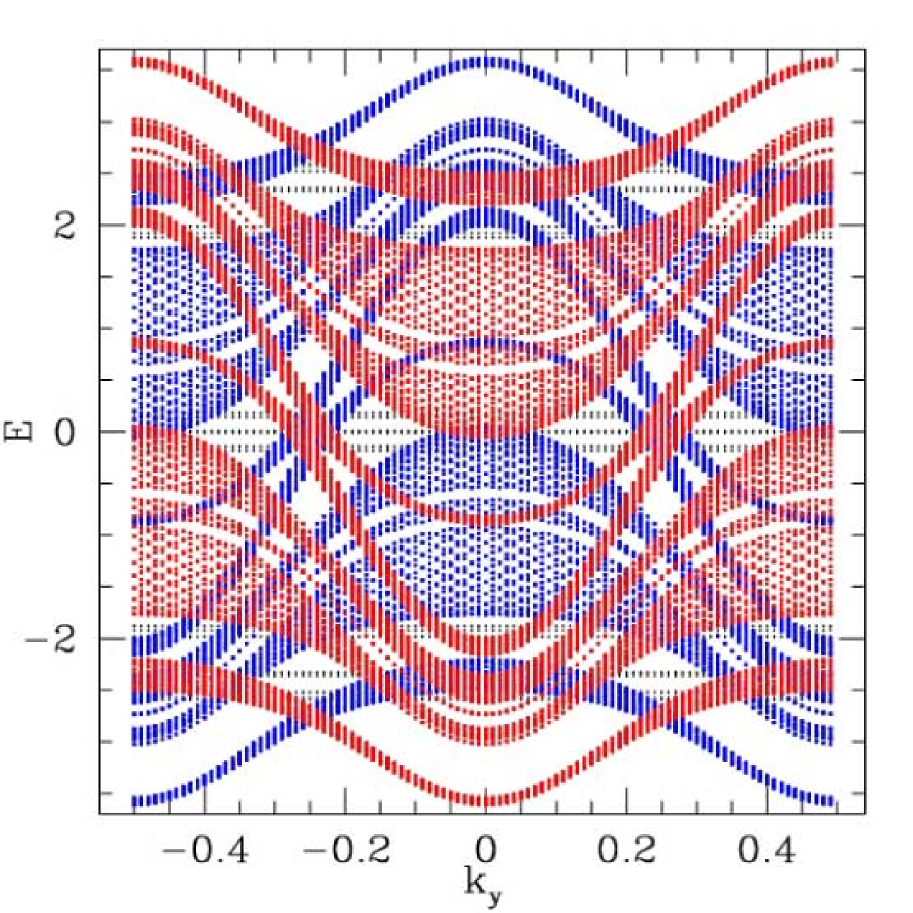
Figure 6: (color online) Energy spectrum viewed as a function of $k_{y}$ for $\alpha_{1}=89/144$ and $\alpha_{2}=\frac{1}{2}$ with $\Lambda=1$ for a range of $k_{x}$ values. The red and blue correspond to $E_{A}$ and $E_{B}$ respectively. The grey dots show the corresponding Abelian case with $\alpha_{1}=\alpha_{2}=\gamma$.

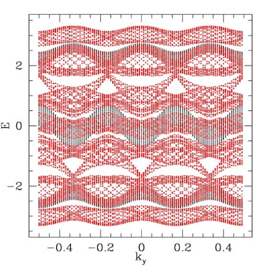
Figure 7: (color online) Energy spectrum viewed as a function of $k_{y}$ for $\alpha_{1}=89/144$ and $\alpha_{2}=\frac{1}{3}$ with $\Lambda=0.5$. The grey dots show a corresponding Abelian case with $\alpha_{1}=\alpha_{2}=\frac{1}{3}$.

For rational $\alpha_{2}=p_{2}/q_{2}$, the spectrum is a periodic function of $k_{y}$. This is due to the fact that for irrational $\alpha_{1}$, the set $\{U_{m}\}$ is ergodic in $m$, while the set $\{V_{m}\}$ is periodic in $m$ for rational $\alpha_{2}$. We list below some of the characteristic properties of the spectrum:

(1) $E_{A,B}(2\pi k_{y})=-E_{A,B}(2\pi k_{y}+2\pi\alpha_{2})$,

(2) $E_{A}(2\pi k_{y})=-E_{B}(2\pi k_{y}+2\pi\alpha_{2})$,

(3) $E_{A,B}(2\pi k_{y})=E_{A,B}(2\pi k_{y}+4\pi\alpha_{2})$,

(4) $E(2\pi k_{y})=E(2\pi k_{y}+4\pi\alpha_{2})$.

For certain values of $\alpha_{2}$, A and B-type of states are degenerate. This happens when the two sets $V_{2m}(k_{y})$ and $V_{2m+1}(-k_{y})$ coincide. This degeneracy occurs when (a) $\alpha_{2}$ is an irrational number and (b) $\alpha_{2}=p/q$ with $q$-odd as $V_{m+qn}(k_{y})=V_{q-m+qn}(-k_{y})$ (where $n$ is an integer and $m<q$). For even $q$, the A and B states are in general non-degenerate. This distinction between the odd and the even cases leads to significant differences between these two cases.

VI The Localization Transition

The metal-insulator transitionSok in 2DEGs in the presence of a magnetic (Abelian) field is a paradigm for the Anderson localization transition. We now discuss the corresponding localization transition that exists in the non-Abelian systems. In contrast to the Abelian case, where all states localize at the same value of the tunneling anisotropy, localization in the non-Abelian case varies throughout the spectrum.

In this section, we will discuss the localization properties of the $E=0$ state a study is relevant for fermionic atoms near half-filling. As shown below, for $\alpha_{2}=\frac{1}{2}$ as well as for $\alpha_{2}=\frac{1}{4}$, the onset to a localization transition can be inferred from the well-known localization characteristics of the Harper equation.

A1: Localization Boundary for $\alpha_{2}=1/2$

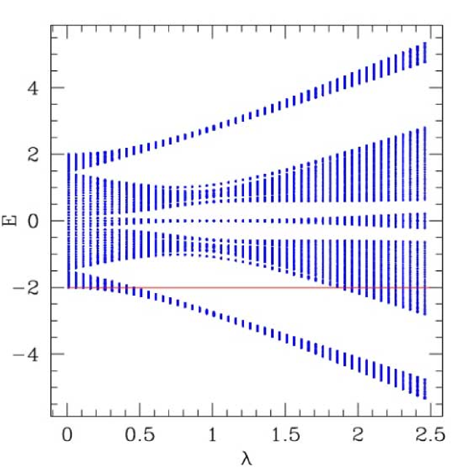
Figure 8: (color online) The eigenvalues of the effective TBM (Eq. (VI)) describing $E=0$ states as $\lambda$ varies. The line (red online) shows the values of $\lambda$ where $E=0$ is an eigenvalue of the TBM (Eq. VI)

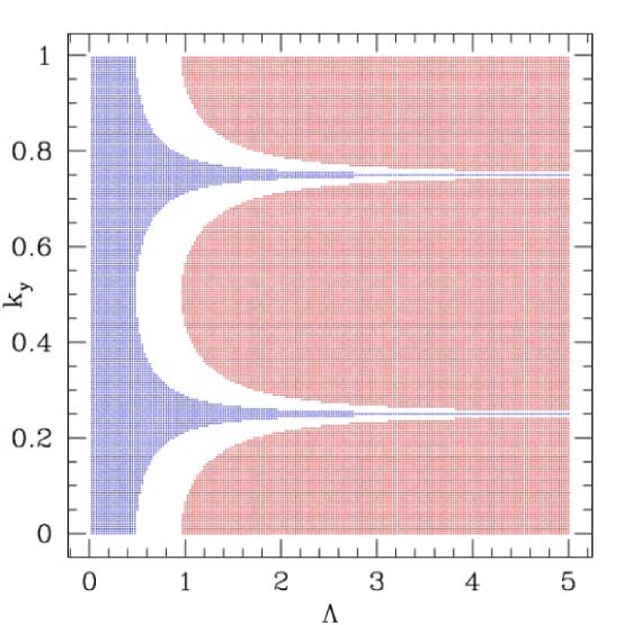
Figure 9: (color online) With $\alpha_{2}=1/2$ shaded regime (blue) shows the extended phase while shaded red shows the localized phase of $E=0$ state in $\Lambda-k_{y}$ plane.

For $\alpha_{2}=\frac{1}{2}$, the coupled TBM equations (Eq.  VI) for $E=0$ reduce to

$$\theta_{m+2}+\theta_{m-2}+2(-1)^{m}\lambda\cos(2\pi\alpha_{1}m-2\pi k_{y})\theta_{m} = \epsilon\theta_{m}$$

$$\eta_{m+1}+\eta_{m-1}+2\Lambda\cos(2\pi\alpha_{1}m-2\pi k_{y})\theta_{m} = 0$$

where $\epsilon=-2$ and $\lambda=2\Lambda^{2}\cos(2\pi k_{y})$.

For $E=0$, the uncoupled $\theta$-equation maps to an $E=-2$ Harper-like equation (Eq. (VI)), where the on-site quasiperiodic potential is a sinusoidal function of $k_{y}$. The eigenstates of this system localize at $\lambda=1$, providing an explicit threshold for localization of the $E=0$ state of the non-Abelian system provided $\epsilon=-2$ is the eigenvalue of Eq. (VI).

As shown in Fig. 8, $\epsilon=-2$ is an eigenvalue of the system provided $\lambda=\lambda_{1}\lesssim 0.48$ or $\lambda=\lambda_{2}\geq 1.83$. These critical values determine the boundary curves for the localization of the $E=0$ state: in the Harper equation, all states are extended for values of $\lambda\leq 1$. These two localization boundaries are exhibited in Fig.  LABEL:locb.2

A2: Localization Boundary for $\alpha_{2}=1/4$

For $\alpha_{2}=\frac{1}{4}$, the uncoupled $\theta$-equations for the A and the B-sectors of the TBM for $E=0$ reduce to

$$\bar{\theta}^{A}_{m+2}+\bar{\theta}^{A}_{m-2}+2i\lambda_{A}\cos(2\pi\alpha_{1}m-2\pi k_{y})\bar{\theta}^{A}_{m} = 0,$$

$$\bar{\theta}^{B}_{m+2}+\bar{\theta}^{B}_{m-2}+2i\lambda_{B}\sin(2\pi\alpha_{1}m-2\pi k_{y})\bar{\theta}^{B}_{m} = 0,$$

where

$$\lambda_{A} = 2\Lambda^{2}\cos(2\pi k_{y}),$$

$$\lambda_{B} = 2\Lambda^{2}\sin(2\pi k_{y}).$$

The above two equations correspond to A and B-type states with $E=0$, respectively. Here $\bar{\theta}_{m}^{A,B}=i^{m}\theta_{m}^{A,B}$. In a manner analogous to the corresponding Hermitian problem, the system exhibits self-duality at $\lambda_{A,B}=1$ and this self-dual point describes the onset of localization Amin . For $k_{y}=\frac{1}{8}$ (mod $\frac{1}{4}$), both types of solutions localize simultaneously. However, at other values of the transverse momentum, only one of the states is localized. This is an example of two degenerate states with different transport properties: depending upon $(\Lambda,k_{y})$, type A states may be extended (localized) while type B states will be localized (extended). This localization boundary in $\Lambda-k_{y}$ space is shown for types A and B in Fig. 10.

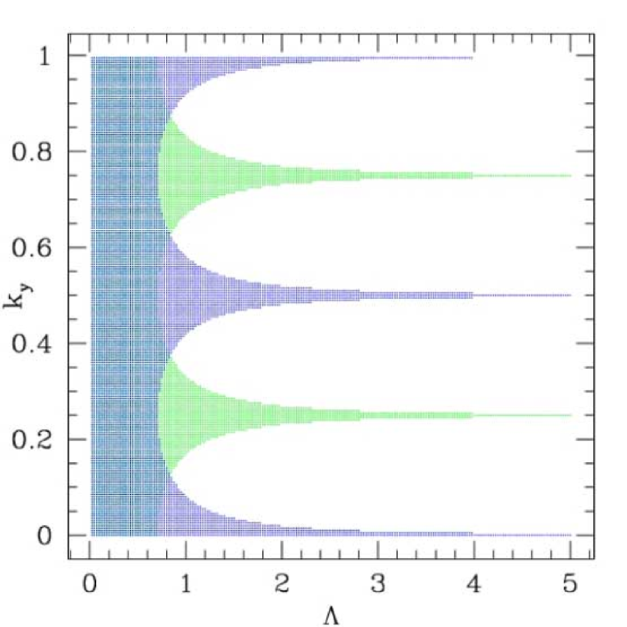
Figure 10: (color online) For $\alpha_{2}=1/4$, shaded regimes show extended phase for two degenerate $E=0$ states belonging to the A (green) and B (blue) sectors in $\Lambda-k_{y}$ plane.

The existence of conducting states for all values of $\Lambda$ is one of the most intriguing characteristics of the non-Abelian system. Below we show that these states defying localization describe relativistic particles.

B: Relativistic Dispersion and Defiance of Localization

Figure 11 shows the energy-momentum relation for $\alpha_{2}=1/2$ near $E=0,k_{y}=1/4$. Although the level structure is complicated, near $k_{y}=1/4$, the energy bands exhibit the linear dispersion characteristic of the one-dimensional relativistic particles. Thus, the non-Abelian system with A and B type states, provides an interesting manifestation of the positive and the negative energy states of a one-dimensional relativistic particle.

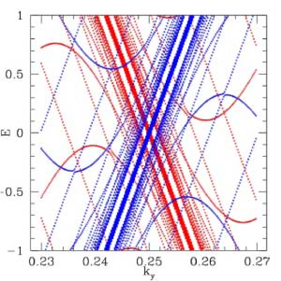
Figure 11: (color online) Blowup of the $E=0$ and $k_{y}=1/4$ neighborhood for $\alpha_{1}=89/144$ and $\alpha_{2}=\frac{1}{2}$ and $\Lambda=10$. The red and blue respectively correspond to $E_{a}$ and $E_{b}$.

An important characteristic of the states that reside at the crossings is that they defy localization. It should be noted that a crossing at $E=0$ exists irrespective of the value of $\Lambda$. In other words, we have a relativistic theory for all values of $\Lambda$ as shown in the Figures 6 and 11. Such states remain extended irrespective of the quasiperiodic disorder in the system as the linear dispersion exists for the full range of $\Lambda$ values.

For $\alpha_{2}=\frac{1}{4}$, we obtain an effective relativistic theory for zero-energy states near $k_{y}=0$ for type-A and near $k_{y}=\pi/2$ for type-B states. These states remain conducting for all values of $\Lambda$.

We would like to note that in the Abelian system, a linear energy-momentum relation resulting in a Dirac cone occurs for rational values of $\alpha$ in the neighborhood of some special values of $k_{x},k_{y}$ near $E=0$. However, for irrational $\alpha$, the spectrum is independent of $k_{y}$ and the Dirac cone disappears. Therefore, in the Abelian case, effective relativistic theory bears no relationship to the transport properties as the states are always extended for rational $\alpha$.

C: Localization Transition and Loss of Relativistic Dispersion

Our detailed investigation for various values of $\alpha_{2}$ shows that the presence of conducting states for all values of $\Lambda$ is not a generic property of the system. In particular, for cases where the type-A and type-B states are always degenerate, all states are found to localize. Interestingly, the transition to localization is accompanied by a loss of the relativistic character of the energy momentum relation.

For example, for $\alpha_{2}=p/q$ where $q$ is odd, as well as for irrational $\alpha_{2}$, the crossings characterizing certain $E=0$ states disappear beyond a certain critical value of $\Lambda$. Interestingly, this threshold for the disappearance of the crossing is always found to coincide with the onset to localization of that state. Figures 12 and 13 illustrate this for irrational $\alpha_{2}$ as the disappearance of band crossings is accompanied by the broadening and flattening of the Bragg peaks.

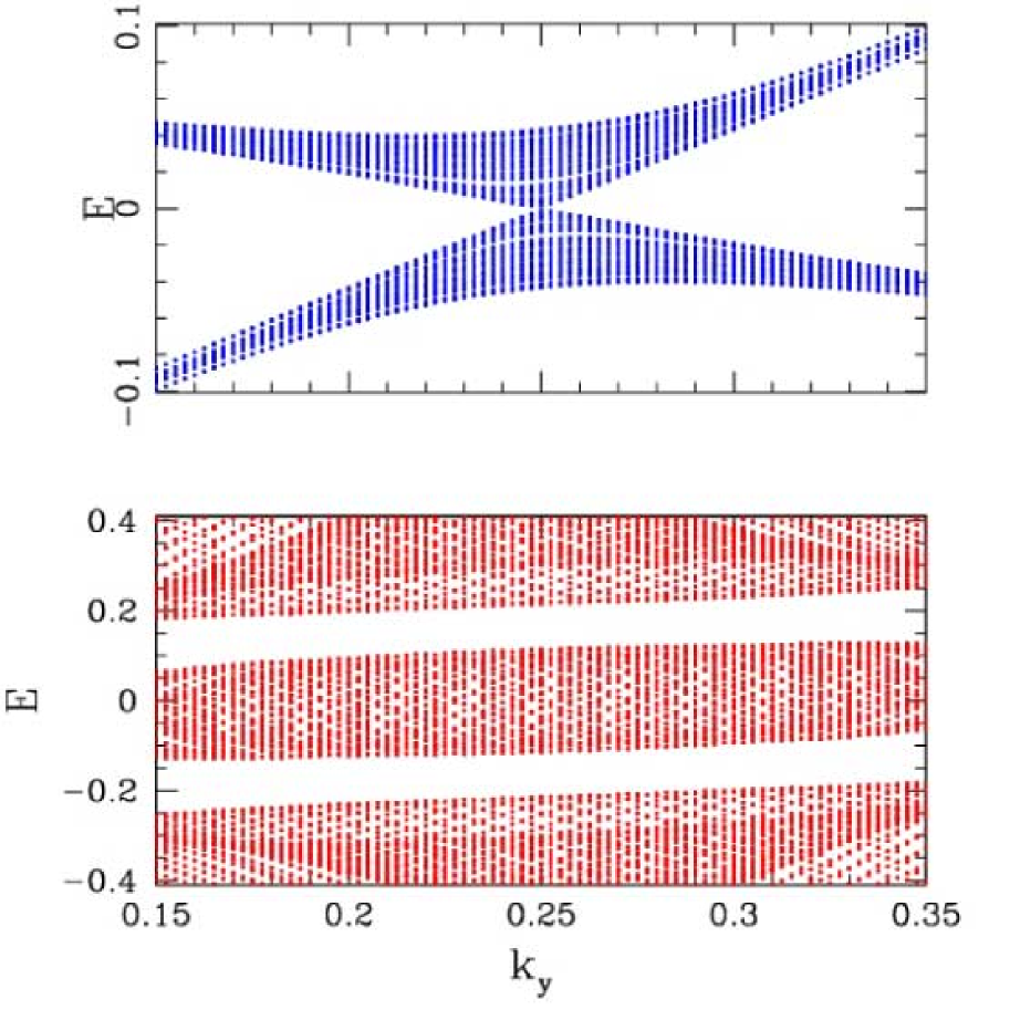
Figure 12: (color online) Top and bottom panel respectively show the spectrum for $\alpha_{2}=\gamma^{3}$ with $\Lambda=0.75,1.25$ which respectively correspond to extended and localized $E=0$ states.

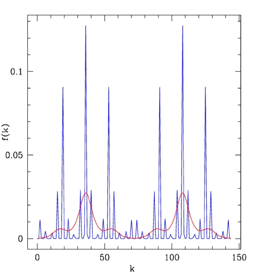
Figure 13: (color online) Fourier transform of the wave function for $E=0$ state with $\alpha_{2}=\gamma^{3}$ with $\Lambda=0.75$ (sharp fringes) and $\Lambda=1.25$ (smeared out fringes). The label $k$ on the x-axis corresponds to the momentum $2\pi k/L$, where $L$ is the size of the lattice.

VII Localization Transition of Bose-Einstein Condensates

The natural locus for BEC in ultracold atoms in optical lattices is the band edge. We now explore the spectral and transport properties of the states at band edges, namely the minimum energy states as $k_{y}$ varies.

In contrast to the preceding analytical treatment of the band centers, we have investigated localization properties of the states at the band edge with numerical methods.

As seen from Figs 6 and 14, the energy spectrum for $\alpha_{2}=\frac{1}{2}$ shows the existence of a linear dispersion relation near the band crossings. As the lattice anisotropy $\Lambda$ varies, we see a transition from relativistic to non-relativistic behavior near $\Lambda\approx 2.5$; this transition is accompanied by the loss of the wave function’s spinor character, causing an effective spin polarization.

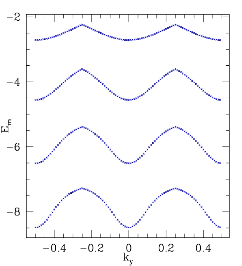
Figure 14: (color online) Minimum energy as a function of $k_{y}$ for $\alpha_{2}=\frac{1}{2}$ with $\Lambda=0.5,1.5,2.5,3.5$ (top-bottom) illustrating the change from linear to quadratic dispersion near $k_{y}=\pm 1/4$.

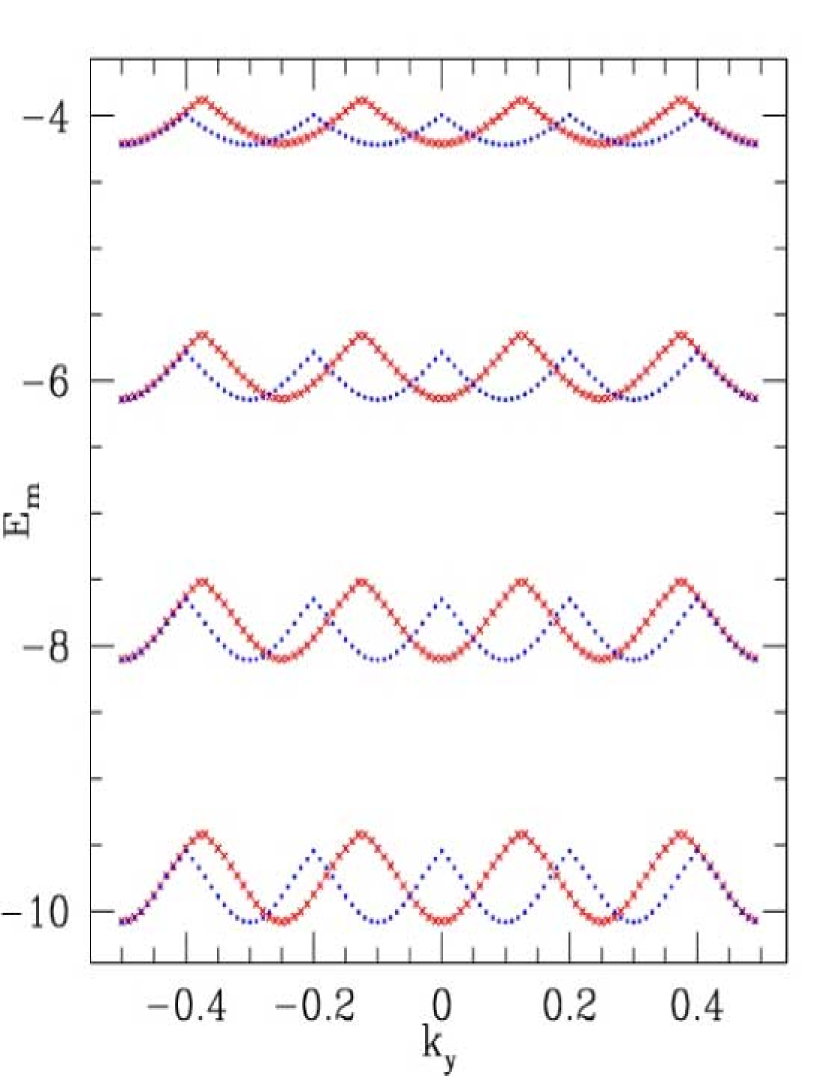
Figure 15: (color online) Minimum energy as a function of $k_{y}$ for $\alpha_{2}=1/4$ (cross), $\alpha_{2}=1/5$ (dots) with $\Lambda=1.5,2.5,3.5,4.5$ (top-bottom) illustrating the change from the linear to quadratic dispersion near $k_{y}=\pm 1/4$.

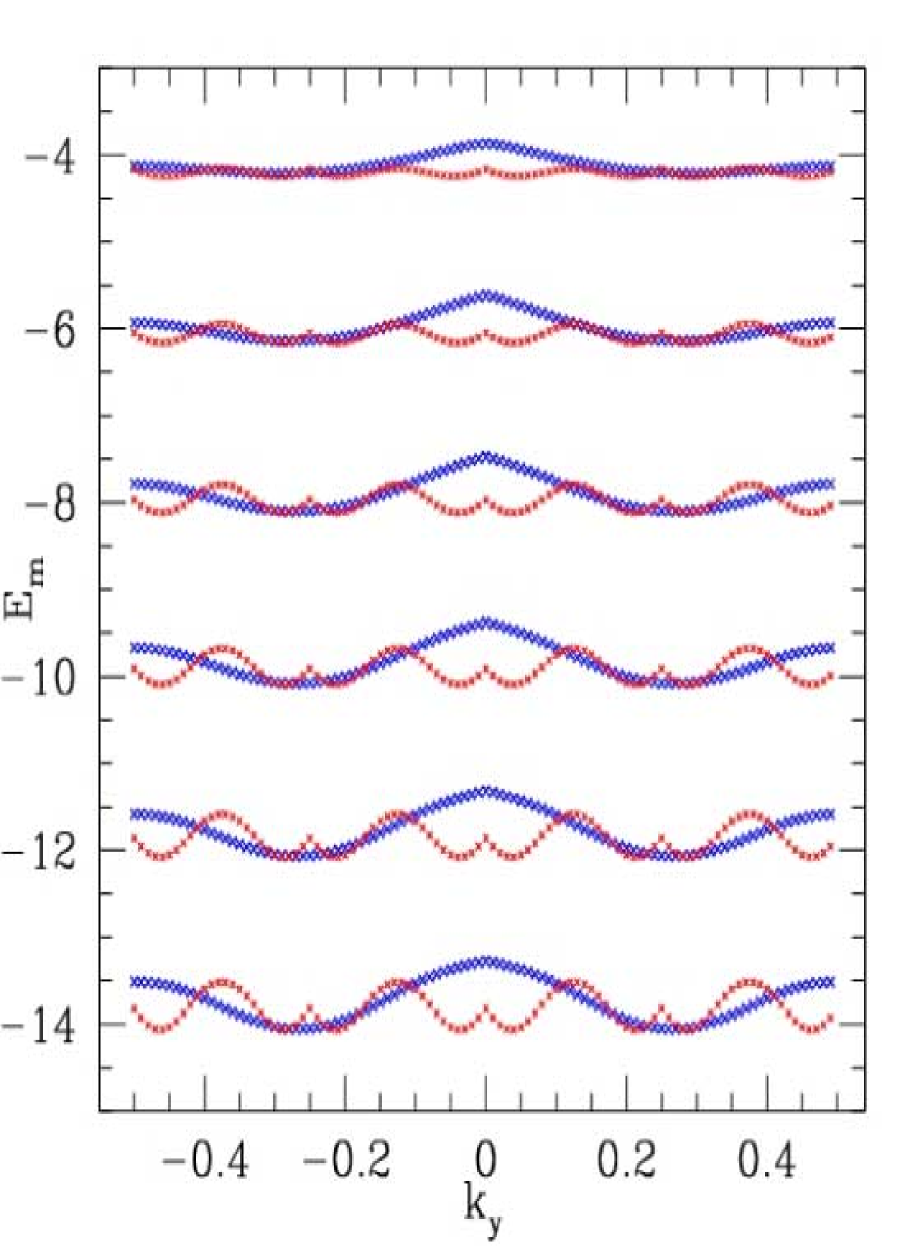
Figure 16: (color online) Variation of minimum energy with $k_{y}$ for $\alpha_{2}=\gamma^{3}$ (large crosses) and $\alpha_{2}=\gamma^{4}$ (smaller crosses) with $\Lambda=1.5,2.5,3.5,4.5,5.5,6.5$ (top-bottom).

The robustness of the linear dispersion in non-Abelian systems is shown for various values of $\alpha_{2}$ in Figs.  15 and  16. It appears that it is only in the even-$q$ cases that the nature of the dispersion changes as $\Lambda$ varies. Similarly, for $\alpha_{2}=\gamma^{4}$ (an odd harmonic of $\gamma$, as $\gamma^{4}=2-3\gamma$), linear dispersion at $k_{y}=0$ and at $k_{y}=1/4$ occurs for all values of $\Lambda$, while for $\alpha_{2}=\gamma^{3}$ (an even harmonic of $\gamma$, as $\gamma^{3}=2\gamma-1$), a relativistic energy-momentum relation is seen for small and large values of $\Lambda$ as illustrated in Fig. 16. In other words, a “transition” from relativistic to non-relativistic behavior can be induced by varying $\Lambda$ for some values of $\alpha_{2}$.

Another point to be noted is that the ground state of the system may have nonzero momentum: for even $q$, the global energy minimum occurs at $k_{y}=0$, while for odd $q$, it occurs at $k_{y}=\alpha_{2}/2$.

Figures 17 illustrate the localization transition of the minimum energy states. Extended states in these figures are characterized by sharp Bragg peaks in the momentum distribution, and the localization transition is signaled by the broadening of these peaks. As we increase the parameter $\Lambda$, the $k_{y}=\pm 1/4$ states localize before the $k_{y}=0$ state. Our detailed investigation shows that $k_{y}=0$ is the last state to localize as $\Lambda$ is varied for all values of $\alpha_{2}$. This is contrary to familiar experience, in which localization begins at the band edge. The localization for the minimum energy state is insensitive to the energy-momentum relation, in contrast to the $E=0$ states.

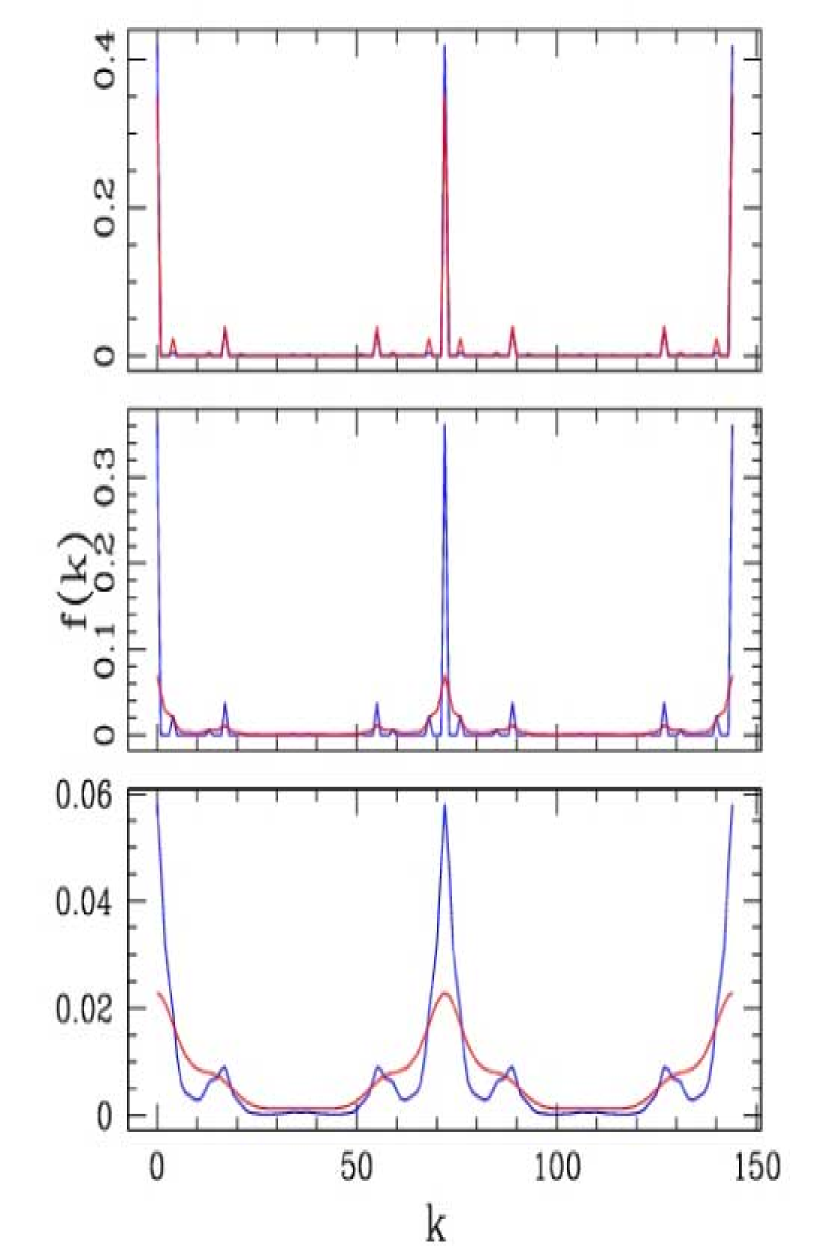
Figure 17: (color online) Fourier transform of the wave function for $\Lambda=.4,.5,.7$ (top-bottom). Each caption shows $k_{y}=.25$(red) and $k_{y}=0$(blue) for the minimum energy state for $\alpha_{2}=1/2$. The x-axis index $k$ corresponds to the Bloch vector $2\pi k/L$. There are peaks corresponding to the irrational values of $\alpha_{1}$, occuring at $k$ values equal to half of the Fibonacci numbers (as anti-ferromagnetic nature effectively doubles the size of the unit cell). Additional satellite peaks characterize the non-Abelian ferature of the system.

For irrational $\alpha_{2}$, we expect the localization threshold to be lowered. Our numerical results show that the minimum energy states begin to localize at a relatively small value of $\Lambda\approx 0.15$. As discussed earlier, $E=0$ states resist localization due to their linear dispersion but eventually localize. Our numerical studies show that localization is complete at $\Lambda=1$, as in the Abelian case.

VIII Experimental Observation of Metal-Insulator Transition

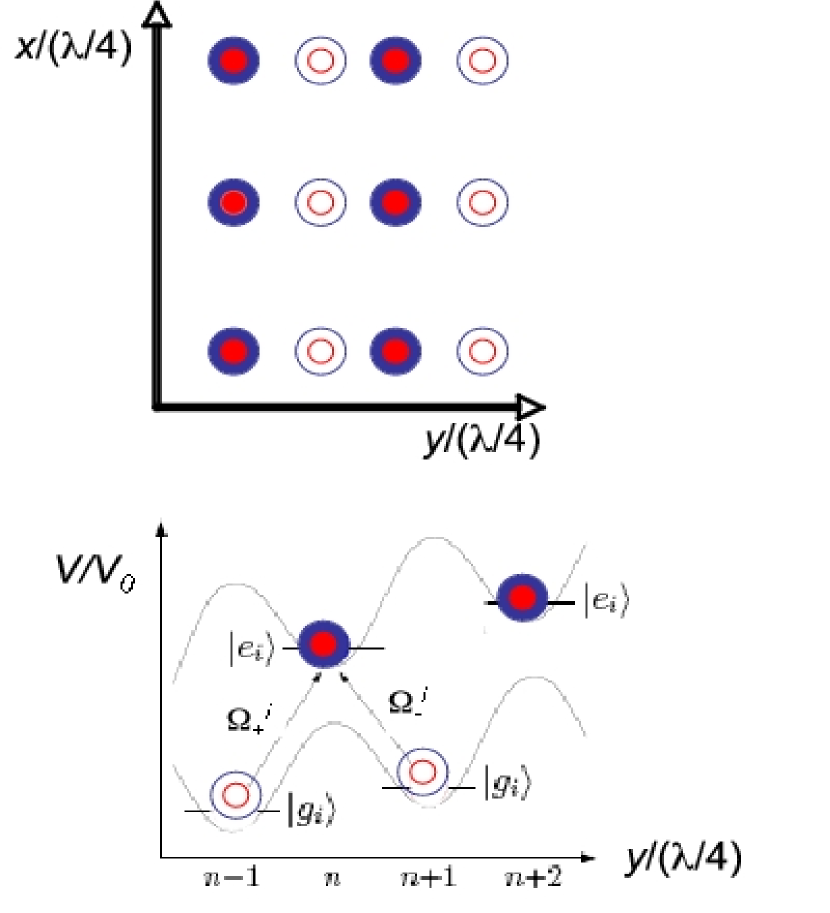
Figure 18: (color online) Schematic diagram illustrating the non-Abelian $U(2)$ set up. The ground states are hollow and the excited states are filled. Red and blue represent the two “colors” of the $U(2)$ group.

An experimental setup for generating artificial Abelian and non-Abelian fields consists of NJP ; NA a two-dimensional optical lattice populated with cold atoms that occupy two hyperfine states. The lattice laser polarization is adjusted to confine these states to alternating columns. The non-Abelian scheme requires atoms with two pairs of hyperfine levels: $|g_{1}\rangle$, $|e_{1}\rangle$, $|g_{2}\rangle$, $|e_{2}\rangle$ as shown in Fig. 18.

The typical kinetic energy tunneling along the $y$-direction is suppressed by accelerating the system or applying an inhomogeneous electric field in that direction such that the lattice is tilted. Tunneling is instead accomplished with two sets of laser-driven Raman transitions with space-dependent Rabi couplings $\Omega_{j}e^{iq_{j}y}$ where $j=1,2$. The wave numbers $q_{j}$ generate an effective magnetic flux where $q_{j}=(2\pi\alpha_{j})/a$, where $\lambda=2a$ is the wavelength of the laser light. In an optical lattice with a finite number of sites, the two components of the ”magnetic flux” ( $\alpha_{1},\alpha_{2}$ ) can be adjusted, in a controlled manner, to a sequence of rational approximants to the golden mean by tuning the $q_{j}$. We direct readers to Refs.NJP ; NA regarding various details for generating these artificial gauge fields.

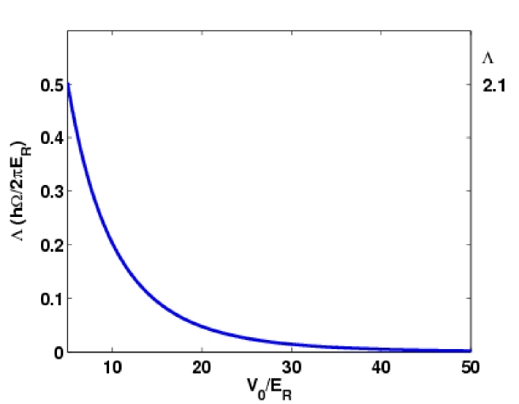
Figure 19: (color online) $\Lambda$ as the depth of the 2D optical lattice is tuned with $\alpha=\frac{1}{2}$. The factor $E_{R}/\hbar\Omega\approx 4.2$ with the following laser parameters: $I_{g}=1$ mW/cm², $x=11$, $\delta_{r}=100$ GHz, $E_{R}/h=3.2$ kHz.

We now describe the experimental feasibility of tuning $\Lambda$ to induce metal-insulator transitions by adjusting the lattice beam intensity $V_{0}$. For simplicity, we will initially discuss the Abelian case. Let us first consider the laser assisted coupling $J_{y}$ as a function of $V_{0}/E_{R}$, where $E_{R}=2\pi^{2}\hbar^{2}/M\lambda^{2}$ is the photon recoil energy. The tunneling is defined as the matrix element of the Rabi coupling ($\Omega$) between Wannier functions $w$, evaluated at the two adjacent lattice sites:

$$J_{y}=\int w(\vec{x}-\vec{x}_{i})\frac{\hbar}{2}\Omega\exp(iqx)w(\vec{x}-\vec{x}_{i-1})d^{3}\vec{x},$$ (36)

where $q=(2\pi\alpha)/a$. The Wannier functions for $V(x)=V_{0}\sin^{2}(2\pi x/\lambda)$] have been computed  NJP ; $J_{y}$ decreases monotonically with $V_{0}/E_{R}$. This basic behavior can be demonstrated analytically by assuming a deep lattice approximated by a harmonic oscillator potential and taking the Wannier functions to have the corresponding Gaussian form. The Gaussian approximation yields

$$J_{y}=\frac{\hbar\Omega}{2}\exp[-\frac{\pi^{2}}{16}\sqrt{V_{0}/E_{R}}]\exp[-\frac{\alpha^{2}}{\sqrt{V_{0}/E_{R}}}].$$ (37)

The kinetic energy coupling in the $x$-direction $J_{x}$ also decreases monotonically with $V_{0}/E_{R}$ for sufficiently large values RPCW as described by

$$J_{x}\approx 1.397E_{R}\left(\frac{V_{0}}{E_{R}}\right)^{1.051}\exp[-2.121\sqrt{V_{0}/E_{R}}].$$ (38)

The ratio of $\Lambda=J_{x}/J_{y}=(E_{R}/\hbar\Omega)\,f(V_{0}/E_{R},\alpha)$ is shown in Fig. 19 for a characteristic range of $V_{0}/E_{R}$ with the scale set by the factor $\hbar\Omega/E_{R}$. In order to generate a useful range of $\Lambda$ values (e.g.,$0<\Lambda\lesssim 2$), the parameter $\hbar\Omega/E_{R}$ must be set to order unity.

We now argue that it is possible to achieve this with reasonable experimental settings. We consider the case of ⁸⁷Rb, where the $|g\rangle$ and $|e\rangle$ states are taken to be the hyperfine levels of the $5^{2}S_{1/2}$ level data and the Raman level is $5^{2}P_{3/2}^{\circ}$. The parameter $\hbar\Omega/E_{R}$ can be fixed near unity if the Raman laser beams have intensities on the order of 1 mW/cm² with $x\approx 11$ and are detuned from the ⁸⁷Rb $D_{2}$ line by about $\delta_{r}\approx 100$ GHz. We require that the Rabi coupling of the Raman transition $\Omega$, the detuning $\Delta$, and the lattice trapping frequency $\nu_{x}=\sqrt{4E_{R}V_{0}}/\hbar$ have well separated magnitudes such that $\Omega\ll\Delta\ll\nu_{x}$, to ensure that only the lowest band of the lattice is occupied and no other excitations occur. Typical values of $\nu_{x}$ are on the order of tens of kilohertz. The Raman transition is stimulated by two lasers with Rabi couplings $\Omega_{g}^{(1)}$ and $\Omega_{e}^{(1)}$ and intensities $I_{g}$ and $I_{e}$ with a large detuning $\delta_{r}$ such that the effective Rabi coupling magnitude is $\Omega=\Omega_{g}^{(1)}\Omega_{e}^{(1)}/2\delta_{r}$. The Rabi coupling $\Omega$ can be written as a product of atomic factors and laser tuning parameters,

$$\Omega=\left(\frac{\Gamma^{2}}{4I_{sat}}\right)\left(\frac{\sqrt{\xi}I_{g}}{\delta_{r}}\right),$$

where $\Gamma$ is the natural decay rate of the $5^{2}P_{3/2}\circ$ state and $I_{sat}$ is the saturation intensity of the $D_{2}$ line (See Ref. data ). The ratio $\xi=I_{e}/I_{g}$ must be less than 0.17 or greater than 5.8 to satisfy the $\Omega\ll\Delta$ condition. The separation of scales between the Rabi coupling $\Omega$ of the Raman transition and lattice trapping frequency $\nu_{x}$ necessary to generate the magnetic field in the above scheme (i.e., $\Omega\ll\nu_{x}$) is sufficient to generate a reasonable range of $\Lambda$ values.

In the non-Abelian case, there are generally two possible values of $\Lambda$ corresponding to $\Omega_{1}$ and $\Omega_{2}$, one for each “color”. By adjusting $\Omega_{2}/\Omega_{1}=f(V_{0}/E_{R},\alpha_{1})/f(V_{0}/E_{R},\alpha_{2})$, we obtain a single $\Lambda$ in correspondence with the theoretical studies described here.

IX Summary

This paper discusses spectral and transport properties of the cold atom analog of a 2DEG in a lattice, subject to a non-Abelian gauge field with $U(2)$ symmetry.

In the continuum limit of the lattice, the system maps onto two oppositely-charged coupled harmonic oscillators, with a coupling constant proportional to the strength of the non-Abelian field. The Landau energy levels of the Abelian problem evolve into entangled states of this particle-hole pair.

These features also characterize the energy spectrum of the the corresponding lattice problem. In fact, the transition from Landau levels to Landau bands is the analog of the generalization from the butterfly to the moth spectrum as the Abelian system becomes non-Abelian. The non-Abelian coupling breaks the degeneracy of the Landau levels; the spectrum depends explicitly on the transverse momentum.

The non-Abelian system exhibits antiferrimagnetic-type ground states, whose components, A and B, need not be degenerate, and in fact may have very different transport properties. A particularly interesting example of this is the zero-energy state for $\alpha_{2}=1/4$, where the degenerate A and B components have different localization properties. Additionally, an intriguing relationship between the A and the B components occurs for $\alpha_{2}=\frac{1}{2}$, as these two components correspond to the positive and the negative energy states of the system. Such novelties may open new avenues for exploring frontiers of physics with cold atoms.

The use of ultracold atoms to simulate relativistic as well as non-relativistic theories and study the effect of disorder is an exciting field of research. In a two-dimensional lattice subject to a non-Abelian gauge field, one can induce not only localization transitions, but also a transition from relativistic to non-relativistic theory by tuning the lattice anisotropy. A well known feature of the Dirac Hamiltonian is an extra term in the conductivity attributed to Zitterbewegung (ZB) ZB corresponding to inter-band transitions. It has been suggested that such a term is responsible for the finite conductivity of graphene described by a massless Dirac energy spectrum ZB . In other words, it is ZB that makes it impossible to localize relativistic particles, as it is connected with the uncertainty of the position of a relativistic quantum particle due to the creation of particle-antiparticle pairs. Therefore, the origin of delocalization characterizing the non-Abelian system that persists even for infinite disorder ($\Lambda\rightarrow\infty$) can be attributed to ZB.

The detection of relativistic particle and a transition from non-relativistic to relativistic dispersion in cold atoms in optical lattices was recently discussed; it was shown that the relativistic dispersion can be detected using atomic density profiles as well as Bragg spectroscopy  duan .

Our detailed study for various values of $\alpha_{2}$ captures some of the universal features of non-Abelian systems. Exploration of the two-dimensional space ($\alpha_{1}$, $\alpha_{2}$) may reveal additional phenomena, and the richness of $U(N)$ gauge systems with $N>2$ remains to be explored. Moreover, the effects of interparticle interactions remain to be investigated gpe .

X Acknowledgment

We are grateful to Ashwin Rastogi for his efforts in initiating the study of the continuum limit of the problem and Jay Hanssen for helpful discussions regarding experimental aspects of this work. We would also like to thank Ian Spielman and Nathan Goldman for their comments and suggestions on the paper.

References

- (1) J. Ruseckas, G. Juzeliunas, P. Ohberg and M. Fleischhauer, Phys. Rev. Lett., 95 010404 (2005).
- (2) D. Jaksch and P. Zoller, New. J. Phys. 5, 56 (2003).
- (3) K. Osterloh, M. Baig, L. Santos, P. Zoller and M. Lewenstein, Phys. Rev. Lett., 95, 010403 (2005).
- (4) Erich J. Mueller, Phys. Rev. A, 70, 041603(R) (2004).
- (5) N. Goldman and P. Gaspard, Europhys. Lett., 78, 60001, (2007).
- (6) See for example, Richard Prange, “The Quantum Hall Effect,” Springer-Verlag, edited by Richard Prange and Steven Girvin, (1990).
- (7) L. Onsanger, Phil. Mag, 43, 1006, (1952).
- (8) P. G. Harper, Phys Soc. A, 68, 879, (1955); S. Aubry and G. Andre, Ann. Isr. Phys. Soc., 3, 133 (1980).
- (9) D. R. Hofstadter, Phys. Rev. B, 14, 2239 (1976).
- (10) K. Drese and M. Holthaus, Phys. Rev. Lett., 78, 2932, (1997).
- (11) For a review, see J. B. Sokoloff, Phys. Rep. 126, 189 (1985).
- (12) Indubala I. Satija, Daniel C. Dakin and Charles W. Clark, Phys. Rev. Lett., 97, 21640 (2006), erratum at 98, 269904 (2007).
- (13) Shi-Liang Zhu, Baigeng Wang and L.M. Duan, Phys. Rev. Lett., 98 260402 (2007).
- (14) L. Balents and M. Fisher, Phys. Rev. B, 56, 12970 (1997).
- (15) Amin Jazeri and Indubala I. Satija, Phys. Rev. E, 63, 036222 (2001).
- (16) M. I. Katsnelson, Eur. Phys. J. B, 51, 157 (2006).
- (17) D. A. Steck, data available at http://steck.us/alkalidata.
- (18) A. M. Rey, G. Pupillo, C. W. Clark and C. J. Williams, Phys. Rev. A 72, 033616, (2005)
- (19) N. Goldman, Europhys. Lett. 80, 20001 (2007).