Eingereicht am 24.11.2006
bei der Fakultät für Physik und Astronomie

1. Gutachter: Prof. Dr. W. Kinzel
2. Gutachter: Prof. Dr. F. Assaad
der Dissertation.
 
1. Prüfer: Prof. Dr. W. Kinzel
2. Prüfer: Prof. Dr. F. Assaad
3. Prüfer: Prof. Dr. P. Jakob
im Promotionskolloquium
 
Tag des Promotionskolloquiums: 18.05.2007
 
Doktorurkunde ausgehändigt am: 20.07.2007

Abstract

Neural networks can synchronize by learning from each other. For that purpose they receive common inputs and exchange their outputs. Adjusting discrete weights according to a suitable learning rule then leads to full synchronization in a finite number of steps. It is also possible to train additional neural networks by using the inputs and outputs generated during this process as examples. Several algorithms for both tasks are presented and analyzed.

In the case of Tree Parity Machines the dynamics of both processes is driven by attractive and repulsive stochastic forces. Thus it can be described well by models based on random walks, which represent either the weights themselves or order parameters of their distribution. However, synchronization is much faster than learning. This effect is caused by different frequencies of attractive and repulsive steps, as only neural networks interacting with each other are able to skip unsuitable inputs. Scaling laws for the number of steps needed for full synchronization and successful learning are derived using analytical models. They indicate that the difference between both processes can be controlled by changing the synaptic depth. In the case of bidirectional interaction the synchronization time increases proportional to the square of this parameter, but it grows exponentially, if information is transmitted in one direction only.

Because of this effect neural synchronization can be used to construct a cryptographic key-exchange protocol. Here the partners benefit from mutual interaction, so that a passive attacker is usually unable to learn the generated key in time. The success probabilities of different attack methods are determined by numerical simulations and scaling laws are derived from the data. If the synaptic depth is increased, the complexity of a successful attack grows exponentially, but there is only a polynomial increase of the effort needed to generate a key. Therefore the partners can reach any desired level of security by choosing suitable parameters. In addition, the entropy of the weight distribution is used to determine the effective number of keys, which are generated in different runs of the key-exchange protocol using the same sequence of input vectors.

If the common random inputs are replaced with queries, synchronization is possible, too. However, the partners have more control over the difficulty of the key exchange and the attacks. Therefore they can improve the security without increasing the average synchronization time.

Zusammenfassung

Neuronale Netze, die die gleichen Eingaben erhalten und ihre Ausgaben austauschen, können voneinander lernen und auf diese Weise synchronisieren. Wenn diskrete Gewichte und eine geeignete Lernregel verwendet werden, kommt es in endlich vielen Schritten zur vollständigen Synchronisation. Mit den dabei erzeugten Beispielen lassen sich weitere neuronale Netze trainieren. Es werden mehrere Algorithmen für beide Aufgaben vorgestellt und untersucht.

Attraktive und repulsive Zufallskräfte treiben bei Tree Parity Machines sowohl den Synchronisationsvorgang als auch die Lernprozesse an, so dass sich alle Abläufe gut durch Random-Walk-Modelle beschreiben lassen. Dabei sind die Random Walks entweder die Gewichte selbst oder Ordnungsparameter ihrer Verteilung. Allerdings sind miteinander wechselwirkende neuronale Netze in der Lage, ungeeignete Eingaben zu überspringen und so repulsive Schritte teilweise zu vermeiden. Deshalb können Tree Parity Machines schneller synchronisieren als lernen. Aus analytischen Modellen abgeleitete Skalengesetze zeigen, dass der Unterschied zwischen beiden Vorgängen von der synaptischen Tiefe abhängt. Wenn die beiden neuronalen Netze sich gegenseitig beeinflussen können, steigt die Synchronisationszeit nur proportional zu diesem Parameter an; sie wächst jedoch exponentiell, sobald die Informationen nur in eine Richtung fließen.

Deswegen lässt sich mittels neuronaler Synchronisation ein kryptographisches Schlüsselaustauschprotokoll realisieren. Da die Partner sich gegenseitig beeinflussen, der Angreifer diese Möglichkeit aber nicht hat, gelingt es ihm meistens nicht, den erzeugten Schlüssel rechtzeitig zu finden. Die Erfolgswahrscheinlichkeiten der verschiedenen Angriffe werden mittels numerischer Simulationen bestimmt. Die dabei gefundenen Skalengesetze zeigen, dass die Komplexität eines erfolgreichen Angriffs exponentiell mit der synaptischen Tiefe ansteigt, aber der Aufwand für den Schlüsselaustausch selbst nur polynomial anwächst. Somit können die Partner jedes beliebige Sicherheitsniveau durch geeignete Wahl der Parameter erreichen. Außerdem wird die effektive Zahl der Schlüssel berechnet, die das Schlüsselaustauschprotokoll bei vorgegebener Zeitreihe der Eingaben erzeugen kann.

Der neuronale Schlüsselaustausch funktioniert auch dann, wenn die Zufallseingaben durch Queries ersetzt werden. Jedoch haben die Partner in diesem Fall mehr Kontrolle über die Komplexität der Synchronisation und der Angriffe. Deshalb gelingt es, die Sicherheit zu verbessern, ohne den Aufwand zu erhöhen.

Inhaltsverzeichnis

1. 1 Introduction
2. 2 Neural synchronization
   1. 2.1 Tree Parity Machines
   2. 2.2 Learning rules
   3. 2.3 Order parameters
   4. 2.4 Neural cryptography
      1. 2.4.1 Simple attack
      2. 2.4.2 Geometric attack
      3. 2.4.3 Majority attack
      4. 2.4.4 Genetic attack
3. 3 Dynamics of the neural synchronization process
   1. 3.1 Effect of the learning rules
      1. 3.1.1 Distribution of the weights
      2. 3.1.2 Attractive and repulsive steps
   2. 3.2 Transition probabilities
      1. 3.2.1 Simple attack
      2. 3.2.2 Synchronization
      3. 3.2.3 Geometric attack
   3. 3.3 Dynamics of the weights
      1. 3.3.1 Waiting time for a reflection
      2. 3.3.2 Synchronization of two random walks
      3. 3.3.3 Probability distribution
      4. 3.3.4 Extreme order statistics
   4. 3.4 Random walk of the overlap
      1. 3.4.1 Synchronization on average
      2. 3.4.2 Synchronization by fluctuations
   5. 3.5 Synchronization time
      1. 3.5.1 Number of hidden units
      2. 3.5.2 Learning rules
4. 4 Security of neural cryptography
   1. 4.1 Success probability
      1. 4.1.1 Attacks using a single neural network
      2. 4.1.2 Genetic attack
      3. 4.1.3 Majority attack
      4. 4.1.4 Comparison of the attacks
   2. 4.2 Security by interaction
      1. 4.2.1 Version space
      2. 4.2.2 Mutual information
   3. 4.3 Number of keys
      1. 4.3.1 Synchronization without interaction
      2. 4.3.2 Effective key length
   4. 4.4 Secret inputs
      1. 4.4.1 Feedback mechanism
      2. 4.4.2 Synchronization with feedback
      3. 4.4.3 Key exchange with authentication
5. 5 Key exchange with queries
   1. 5.1 Queries
   2. 5.2 Synchronization time
   3. 5.3 Security against known attacks
      1. 5.3.1 Dynamics of the overlap
      2. 5.3.2 Success probability
      3. 5.3.3 Optimal local field
      4. 5.3.4 Genetic attack
      5. 5.3.5 Comparison of the attacks
   4. 5.4 Possible security risks
      1. 5.4.1 Known local field
      2. 5.4.2 Information about weight vectors
6. 6 Conclusions and outlook
7. A Notation
8. B Iterative calculation
   1. B.1 Local field and output bits
   2. B.2 Equations of motion
9. C Generation of queries

Kapitel 1 Introduction

Synchronization is an interesting phenomenon, which can be observed in a lot of physical and also biological systems [1]. It has been first discovered for weakly coupled oscillators, which develop a constant phase relation to each other. While a lot of systems show this type of synchronization, a periodic time evolution is not required. This is clearly visible in the case of chaotic systems. These can be synchronized by a common source of noise [2, 3] or by interaction [4, 5].

As soon as full synchronization is achieved, one observes two or more systems with identical dynamics. But sometimes only parts synchronize. And it is even possible that one finds a fixed relation between the states of the systems instead of identical dynamics. Thus these phenomena look very different, although they are all some kind of synchronization. In most situations it does not matter, if the interaction is unidirectional or bidirectional. So there is usually no difference between components, which influence each other actively and those which are passively influenced by the dynamics of other systems.

Recently it has been discovered that artificial neural networks can synchronize, too [6, 7]. These mathematical models have been first developed to study and simulate the behavior of biological neurons. But it was soon discovered that complex problems in computer science can be solved by using neural networks. This is especially true if there is little information about the problem available. In this case the development of a conventional algorithm is very difficult or even impossible. In contrast, neural networks have the ability to learn from examples. That is why one does not have to know the exact rule in order to train a neural network. In fact, it is sufficient to give some examples of the desired classification and the network takes care of the generalization. Several methods and applications of neural networks can be found in [8].

A feed-forward neural network defines a mapping between its input vector $\mathbf{x}$ and one or more output values $\sigma_{i}$. Of course, this mapping is not fixed, but can be changed by adjusting the weight vector $\mathbf{w}$, which defines the influence of each input value on the output. For the update of the weights there are two basic algorithms possible: In batch learning all examples are presented at the same time and then an optimal weight vector is calculated. Obviously, this only works for static rules. But in online learning only one example is used in each time step. Therefore it is possible to train a neural network using dynamical rules, which change over time. Thus the examples can be generated by another neural network, which adjusts its weights, too.

This approach leads to interacting neural feed-forward networks, which synchronize by mutual learning [6]. They receive common input vectors and are trained using the outputs of the other networks. After a short time full synchronization is reached and one observes either parallel or anti-parallel weight vectors, which stay synchronized, although they move in time. Similar to other systems there is no obvious difference between unidirectional and bidirectional interaction in the case of simple perceptrons [9].

But Tree Parity Machines, which are more complex neural networks with a special structure, show a new phenomenon. Synchronization by mutual learning is much faster than learning by adapting to examples generated by other networks [10, 11, 9, 12]. Therefore one can distinguish active and passive participants in such a communication. This allows for new applications, which are not possible with the systems known before. Especially the idea to use neural synchronization for a cryptographic key-exchange protocol, which has been first proposed in [13], has stimulated most research in this area [10, 9, 12, 11, 14, 15, 16, 17, 18, 19, 20, 21, 22, 23, 24].

Abbildung 1.1: Key exchange between two partners with a passive attacker listening to the communication.

Such an algorithm can be used to solve a common cryptographic problem [25]: Two partners Alice and Bob want to exchange secret messages over a public channel. In order to protect the content against an opponent Eve, A encrypts her message using a fast symmetric encryption algorithm. But now B needs to know A’s key for reading her message. This situation is depicted in figure 1.1.

In fact, there are three possible solutions for this key-exchange problem [26]. First A and B could use a second private channel to transmit the key, e. g. they could meet in person for this purpose. But usually this is very difficult or just impossible. Alternatively, the partners can use public-key cryptography. Here an asymmetric encryption algorithm is employed so that the public keys of A’s and B’s key pair can be exchanged between the partners without the need to keep them secret. But asymmetric encryption is much slower than symmetric algorithms. That is why it is only used to transmit a symmetric session key. However, one can achieve the same result by using a key-exchange protocol. In this case messages are transmitted over the public channel and afterwards A and B generate a secret key based on the exchanged information. But E is unable to discover the key because listening to the communication is not sufficient.

Such a protocol can be constructed using neural synchronization [13]. Two Tree Parity Machines, one for A and one for B respectively, start with random initial weights, which are kept secret. In each step a new random input vector is generated publicly. Then the partners calculate the output of their neural networks and send it to each other. Afterwards the weight vectors are updated according to a suitable learning rule. Because both inputs and weights are discrete, this procedure leads to full synchronization, $\mathbf{w}_{i}^{A}=\mathbf{w}_{i}^{B}$, after a finite number of steps. Then A and B can use the weight vectors as a common secret key.

In this case the difference between unidirectional learning and bidirectional synchronization is essential for the security of the cryptographic application. As E cannot influence A and B, she is usually not able to achieve synchronization by the time A and B finish generating the key and stop the transmission of the output bits [10]. Consequently, attacks based on learning have only a small probability of success [16]. But using other methods is difficult, too. After all the attacker does not know the internal representation of the multi-layer neural networks. In contrast, it is easy to reconstruct the learning process of a perceptron exactly due to the lack of hidden units. This corresponds with the observation that E is nearly always successful, if these simple networks are used [9].

Of course, one wants to compare the level of security achieved by the neural key-exchange protocol with other algorithms for key exchange. For that purpose some assumptions are necessary, which are standard for all cryptographic systems:

• The attacker E knows all the messages exchanged between A and B. Thus each participant has the same amount of information about all the others. Furthermore the security of the neural key-exchange protocol does not depend on some special properties of the transmission channel.

• E is unable to change the messages, so that only passive attacks are considered. In order to achieve security against active methods, e. g. man-in-the-middle attacks, one has to implement additional provisions for authentication.

• The algorithm is public, because keeping it secret does not improve the security at all, but prevents cryptographic analysis. Although vulnerabilities may not be revealed, if one uses security by obscurity, an attacker can find them nevertheless.

In chapter 2 the basic algorithm for neural synchronization is explained. Definitions of the order parameters used to analyze this effect can be found there, too. Additionally, it contains descriptions of all known methods for E’s attacks on the neural key-exchange protocol.

Then the dynamics of neural synchronization is discussed in chapter 3. It is shown that it is, in fact, a complex process driven by stochastic attractive and repulsive forces, whose properties depend on the chosen parameters. Looking especially at the average change of the overlap between corresponding hidden units in A’s, B’s and E’s Tree Parity Machine reveals the differences between bidirectional and unidirectional interaction clearly.

Chapter 4 focuses on the security of the neural key-exchange protocol, which is essential for this application of neural synchronization. Of course, simulations of cryptographic useful systems do not show successful attacks and the other way round. That is why finding scaling laws in regard to effort and security is very important. As these relations can be used to extrapolate reliably, they play a major role here.

Finally, chapter 5 presents a modification of the neural key-exchange protocol: Queries generated by A and B replace the random sequence of input vectors. Thus the partners have more influence on the process of synchronization, because they are able to control the frequency of repulsive steps as a function of the overlap. In doing so, A and B can improve the security of the neural key-exchange protocol without increasing the synchronization time.

Kapitel 2 Neural synchronization

Synchronization of neural networks [6, 7, 10, 11, 9] is a special case of an online learning situation. Two neural networks start with randomly chosen weight vectors. In each time step they receive a common input vector, calculate their outputs, and communicate them to each other. If they agree on the mapping between the current input and the output, their weights are updated according to a suitable learning rule.

In the case of discrete weight values this process leads to full synchronization in a finite number of steps [9, 10, 12, 11, 27]. Afterwards corresponding weights in both networks have the same value, even if they are updated by further applications of the learning rule. Thus full synchronization is an absorbing state.

Additionally, a third neural network can be trained using the examples, input vectors and output values, generated by the process of synchronization. As this neural network cannot influence the others, it corresponds to a student network which tries to learn a time dependent mapping between inputs and outputs.

In the case of perceptrons, which are simple neural networks, one cannot find any significant difference between these two situations: the average number of steps needed for synchronization and learning is the same [6, 7]. But in the case of the more complex Tree Parity Machines an interesting phenomenon can be observed: two neural networks learning from each other synchronize faster than a third network only listening to the communication [10, 9, 12, 11].

This difference between bidirectional and unidirectional interaction can be used to solve the cryptographic key-exchange problem [13]. For that purpose the partners A and B synchronize their Tree Parity Machines. In doing so they generate their common session key faster than an attacker is able to discover it by training another neural network. Consequently, the difference between synchronization and learning is essential for the security of the neural key-exchange protocol.

In this chapter the basic framework for neural synchronization is presented. This includes the structure of the networks, the learning rules, and the quantities used to describe the process of synchronization.

2.1 Tree Parity Machines

Tree Parity Machines, which are used by partners and attackers in neural cryptography, are multi-layer feed-forward networks. Their general structure is shown in figure 2.1.

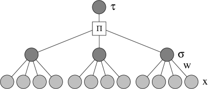
Abbildung 2.1: A Tree Parity Machine with $K=3$ and $N=4$.

Such a neural network consists of $K$ hidden units, which are perceptrons with independent receptive fields. Each one has $N$ input neurons and one output neuron. All input values are binary,

$$x_{i,j}\in\{-1,+1\}\,,$$ (2.1)

and the weights, which define the mapping from input to output, are discrete numbers between $-L$ and $+L$,

$$w_{i,j}\in\{-L,-L+1,\dots,+L\}\,.$$ (2.2)

Here the index $i=1,\dots,K$ denotes the $i$-th hidden unit of the Tree Parity Machine and $j=1,\dots,N$ the elements of the vector.

As in other neural networks the weighted sum over the current input values is used to determine the output of the hidden units. Therefore the full state of each hidden neuron is given by its local field

$$h_{i}=\frac{1}{\sqrt{N}}\mathbf{w}_{i}\cdot\mathbf{x}_{i}=\frac{1}{\sqrt{N}}\sum_{j=1}^{N}w_{i,j}\,x_{i,j}\,.$$ (2.3)

The output $\sigma_{i}$ of the $i$-th hidden unit is then defined as the sign of $h_{i}$,

$$\sigma_{i}=\mathrm{sgn}(h_{i})\,,$$ (2.4)

but the special case $h_{i}=0$ is mapped to $\sigma_{i}=-1$ in order to ensure a binary output value. Thus a hidden unit is only active, $\sigma_{i}=+1$, if the weighted sum over its inputs is positive, otherwise it is inactive, $\sigma_{i}=-1$.

Then the total output $\tau$ of a Tree Parity Machine is given by the product (parity) of the hidden units,

$$\tau=\prod_{i=1}^{K}\sigma_{i}\,,$$ (2.5)

so that $\tau$ only indicates, if the number of inactive hidden units, with $\sigma_{i}=-1$, is even ($\tau=+1$) or odd ($\tau=-1$). Consequently, there are $2^{K-1}$ different internal representations $(\sigma_{1},\sigma_{2},\dots,\sigma_{K})$, which lead to the same output value $\tau$.

If there is only one hidden unit, $\tau$ is equal to $\sigma_{1}$. Consequently, a Tree Parity Machine with $K=1$ shows the same behavior as a perceptron, which can be regarded as a special case of the more complex neural network.

2.2 Learning rules

At the beginning of the synchronization process A’s and B’s Tree Parity Machines start with randomly chosen and therefore uncorrelated weight vectors $\mathbf{w}^{A/B}_{i}$. In each time step $K$ public input vectors $\mathbf{x}_{i}$ are generated randomly and the corresponding output bits $\tau^{A/B}$ are calculated.

Afterwards A and B communicate their output bits to each other. If they disagree, $\tau^{A}\not=\tau^{B}$, the weights are not changed. Otherwise one of the following learning rules suitable for synchronization is applied:

• In the case of the Hebbian learning rule [16] both neural networks learn from each other:

  $$w_{i,j}^{+}=g(w_{i,j}+x_{i,j}\tau\Theta(\sigma_{i}\tau)\Theta(\tau^{A}\tau^{B}))\,.$$ (2.6)

• It is also possible that both networks are trained with the opposite of their own output. This is achieved by using the anti-Hebbian learning rule [11]:

  $$w_{i,j}^{+}=g(w_{i,j}-x_{i,j}\tau\Theta(\sigma_{i}\tau)\Theta(\tau^{A}\tau^{B}))\,.$$ (2.7)

• But the set value of the output is not important for synchronization as long as it is the same for all participating neural networks. That is why one can use the random-walk learning rule [12], too:

  $$w_{i,j}^{+}=g(w_{i,j}+x_{i,j}\Theta(\sigma_{i}\tau)\Theta(\tau^{A}\tau^{B}))\,.$$ (2.8)

In any way only weights are changed by these learning rules, which are in hidden units with $\sigma_{i}=\tau$. By doing so it is impossible to tell which weights are updated without knowing the internal representation $(\sigma_{1},\sigma_{2},\dots,\sigma_{K})$. This feature is especially needed for the cryptographic application of neural synchronization.

Of course, the learning rules have to assure that the weights stay in the allowed range between $-L$ and $+L$. If any weight moves outside this region, it is reset to the nearest boundary value $\pm L$. This is achieved by the function $g(w)$ in each learning rule:

$$g(w)=\left\{\begin{array}[]{cl}\mathrm{sgn}(w)\,L&\mbox{ for $|w|>L$ }\\ w&\mbox{ otherwise }\\ \end{array}\right.\,.$$ (2.9)

Afterwards the current synchronization step is finished. This process can be repeated until corresponding weights in A’s and B’s Tree Parity Machine have equal values, $\mathbf{w}_{i}^{A}=\mathbf{w}_{i}^{B}$. Further applications of the learning rule are unable to destroy this synchronization, because the movements of the weights depend only on the inputs and weights, which are then identical in A’s and B’s neural networks.

2.3 Order parameters

In order to describe the correlations between two Tree Parity Machines caused by the synchronization process, one can look at the probability distribution of the weight values in each hidden unit. It is given by $(2L+1)$ variables

$$p_{a,b}^{i}=P(w_{i,j}^{A}=a\wedge w_{i,j}^{B}=b)\,,$$ (2.10)

which are defined as the probability to find a weight with $w_{i,j}^{A}=a$ in A’s Tree Parity Machine and $w_{i,j}^{B}=b$ in B’s neural network.

While these probabilities are only approximately given as relative frequencies in simulations with finite $N$, their development can be calculated using exact equations of motion in the limit $N\rightarrow\infty$ [17, 18, 19]. This method is explained in detail in appendix B.

In both cases, simulation and iterative calculation, the standard order parameters [28], which are also used for the analysis of online learning, can be calculated as functions of $p_{a,b}^{i}$:

$$Q_{i}^{A}= \displaystyle\frac{1}{N}\mathbf{w}_{i}^{A}\mathbf{w}_{i}^{A} =\sum_{a=-L}^{L}\sum_{b=-L}^{L}a^{2}\,p_{a,b}^{i}\,,$$ (2.11)

$$Q_{i}^{B}= \displaystyle\frac{1}{N}\mathbf{w}_{i}^{B}\mathbf{w}_{i}^{B} =\sum_{a=-L}^{L}\sum_{b=-L}^{L}b^{2}\,p_{a,b}^{i}\,,$$ (2.12)

$$R_{i}^{AB}= \displaystyle\frac{1}{N}\mathbf{w}_{i}^{A}\mathbf{w}_{i}^{B} =\sum_{a=-L}^{L}\sum_{b=-L}^{L}a\,b\,p_{a,b}^{i}\,.$$ (2.13)

Then the level of synchronization is given by the normalized overlap [28] between two corresponding hidden units:

$$\rho_{i}^{AB}=\frac{\mathbf{w}_{i}^{A}\cdot\mathbf{w}_{i}^{B}}{\sqrt{\mathbf{w}_{i}^{A}\cdot\mathbf{w}_{i}^{A}}\sqrt{\mathbf{w}_{i}^{B}\cdot\mathbf{w}_{i}^{B}}}=\frac{R_{i}^{AB}}{\sqrt{Q_{i}^{A}Q_{i}^{B}}}\,.$$ (2.14)

Uncorrelated hidden units, e. g. at the beginning of the synchronization process, have $\rho_{i}=0$, while the maximum value $\rho_{i}=1$ is reached for fully synchronized weights. Consequently, $\rho_{i}$ is the most important quantity for analyzing the process of synchronization.

But it is also interesting to estimate the mutual information gained by the partners during the process of synchronization. For this purpose one has to calculate the entropy [29]

$$S_{i}^{AB}=-N\sum_{a=-L}^{L}\sum_{b=-L}^{L}p_{a,b}^{i}\ln p_{a,b}^{i}$$ (2.15)

of the joint weight distribution of A’s and B’s neural networks. Similarly the entropy of the weights in a single hidden unit is given by

$$S_{i}^{A} = -N\sum_{a=-L}^{L}\left(\sum_{b=-L}^{L}p_{a,b}^{i}\right)\ln\left(\sum_{b=-L}^{L}p_{a,b}^{i}\right)\,,$$ (2.16)

$$S_{i}^{B} = -N\sum_{b=-L}^{L}\left(\sum_{a=-L}^{L}p_{a,b}^{i}\right)\ln\left(\sum_{a=-L}^{L}p_{a,b}^{i}\right)\,.$$ (2.17)

Of course, these equations assume that there are no correlations between different weights in one hidden unit. This is correct in the limit $N\rightarrow\infty$, but not necessarily for small systems.

Using (2.15), (2.16), and (2.17) the mutual information [29] of A’s and B’s Tree Parity Machines can be calculated as

$$I^{AB}=\sum_{i=1}^{K}\left(S_{i}^{A}+S_{i}^{B}-S_{i}^{AB}\right)\,.$$ (2.18)

At the beginning of the synchronization process, the partners only know the weight configuration of their own neural network, so that $I^{AB}=0$. But for fully synchronized weight vectors this quantity is equal to the entropy of a single Tree Parity Machine, which is given by

$$S_{0}=KN\ln(2L+1)$$ (2.19)

in the case of uniformly distributed weights.

2.4 Neural cryptography

The neural key-exchange protocol [13] is an application of neural synchronization. Both partners A and B use a Tree Parity Machine with the same structure. The parameters $K$, $L$ and $N$ are public. Each neural network starts with randomly chosen weight vectors. These initial conditions are kept secret. During the synchronization process, which is described in section 2.2, only the input vectors $\mathbf{x}_{i}$ and the total outputs $\tau^{A}$, $\tau^{B}$ are transmitted over the public channel. Therefore each participant just knows the internal representation $(\sigma_{1},\sigma_{2},\dots,\sigma_{K})$ of his own Tree Parity Machine. Keeping this information secret is essential for the security of the key-exchange protocol. After achieving full synchronization A and B use the weight vectors as common secret key.

The main problem of the attacker E is that the internal representations $(\sigma_{1},\sigma_{2},\dots,\sigma_{K})$ of A’s and B’s Tree Parity Machines are not known to her. As the movement of the weights depends on $\sigma_{i}$, it is important for a successful attack to guess the state of the hidden units correctly. Of course, most known attacks use this approach. But there are other possibilities and it is indeed possible that a clever attack method will be found, which breaks the security of neural cryptography completely. However, this risk exists for all cryptographic algorithms except the one-time pad.

2.4.1 Simple attack

For the simple attack [13] E just trains a third Tree Parity Machine with the examples consisting of input vectors $\mathbf{x}_{i}$ and output bits $\tau^{A}$. These can be obtained easily by intercepting the messages transmitted by the partners over the public channel. E’s neural network has the same structure as A’s and B’s and starts with random initial weights, too.

In each time step the attacker calculates the output of her neural network. Afterwards E uses the same learning rule as the partners, but $\tau^{E}$ is replaced by $\tau^{A}$. Thus the update of the weights is given by one of the following equations:

• Hebbian learning rule:

  $$w_{i,j}^{E+}=g(w_{i,j}^{E}+x_{i,j}\tau^{A}\Theta(\sigma_{i}^{E}\tau^{A})\Theta(\tau^{A}\tau^{B}))\,.$$ (2.20)

• Anti-Hebbian learning rule:

  $$w_{i,j}^{E+}=g(w_{i,j}^{E}-x_{i,j}\tau^{A}\Theta(\sigma_{i}^{E}\tau^{A})\Theta(\tau^{A}\tau^{B}))\,.$$ (2.21)

• Random walk learning rule:

  $$w_{i,j}^{E+}=g(w_{i,j}^{E}+x_{i,j}\Theta(\sigma_{i}^{E}\tau^{A})\Theta(\tau^{A}\tau^{B}))\,.$$ (2.22)

So E uses the internal representation $(\sigma_{1}^{E},\sigma_{2}^{E},\dots,\sigma_{K}^{E})$ of her own network in order to estimate A’s, even if the total output is different. As $\tau^{A}\not=\tau^{E}$ indicates that there is at least one hidden unit with $\sigma_{i}^{A}\not=\sigma_{i}^{E}$, this is certainly not the best algorithm available for an attacker.

2.4.2 Geometric attack

The geometric attack [20] performs better than the simple attack, because E takes $\tau^{E}$ and the local fields of her hidden units into account. In fact, it is the most successful method for an attacker using only a single Tree Parity Machine.

Similar to the simple attack E tries to imitate B without being able to interact with A. As long as $\tau^{A}=\tau^{E}$, this can be done by just applying the same learning rule as the partners A and B. But in the case of $\tau^{E}\not=\tau^{A}$ E cannot stop A’s update of the weights. Instead the attacker tries to correct the internal representation of her own Tree Parity Machine using the local fields $h_{1}^{E}$, $h_{2}^{E}$, …, $h_{K}^{E}$ as additional information. These quantities can be used to determine the level of confidence associated with the output of each hidden unit [30]. As a low absolute value $|h_{i}^{E}|$ indicates a high probability of $\sigma_{i}^{A}\not=\sigma_{i}^{E}$, the attacker changes the output $\sigma_{i}^{E}$ of the hidden unit with minimal $|h_{i}^{E}|$ and the total output $\tau^{E}$ before applying the learning rule.

Of course, the geometric attack does not always succeed in estimating the internal representation of A’s Tree Parity Machine correctly. Sometimes there are several hidden units with $\sigma_{i}^{A}\not=\sigma_{i}^{E}$. In this case the change of one output bit is not enough. It is also possible that $\sigma_{i}^{A}=\sigma_{i}^{E}$ for the hidden unit with minimal $|h_{i}^{E}|$, so that the geometric correction makes the result worse than before.

2.4.3 Majority attack

With the majority attack [21] E can improve her ability to predict the internal representation of A’s neural network. For that purpose the attacker uses an ensemble of $M$ Tree Parity Machines instead of a single neural network. At the beginning of the synchronization process the weight vectors of all attacking networks are chosen randomly, so that their average overlap is zero.

Similar to other attacks, E does not change the weights in time steps with $\tau^{A}\not=\tau^{B}$, because the partners skip these input vectors, too. But for $\tau^{A}=\tau^{B}$ an update is necessary and the attacker calculates the output bits $\tau^{E,m}$ of her Tree Parity Machines. If the output bit $\tau^{E,m}$ of the $m$-th attacking network disagrees with $\tau^{A}$, E searches the hidden unit $i$ with minimal absolute local field $|h_{i}^{E,m}|$. Then the output bits $\sigma_{i}^{E,m}$ and $\tau^{E,m}$ are inverted similarly to the geometric attack. Afterwards the attacker counts the internal representations $(\sigma^{E,m}_{1},\dots,\sigma^{E,m}_{K})$ of her Tree Parity Machines and selects the most common one. This majority vote is then adopted by all attacking networks for the application of the learning rule.

But these identical updates create and amplify correlations between E’s Tree Parity Machines, which reduce the efficiency of the majority attack. Especially if the attacking neural networks become fully synchronized, this method is reduced to a geometric attack.

In order to keep the Tree Parity Machines as uncorrelated as possible, majority attack and geometric attack are used alternately [21]. In even time steps the majority vote is used for learning, but otherwise E only applies the geometric correction. Therefore not all updates of the weight vectors are identical, so that the overlap between them is reduced. Additionally, E replaces the majority attack by the geometric attack in the first $100$ time steps of the synchronization process.

2.4.4 Genetic attack

The genetic attack [22] offers an alternative approach for the opponent, which is not based on optimizing the prediction of the internal representation, but on an evolutionary algorithm. E starts with only one randomly initialized Tree Parity Machine, but she can use up to $M$ neural networks.

Whenever the partners update the weights because of $\tau^{A}=\tau^{B}$ in a time step, the following genetic algorithm is applied:

• As long as E has at most $M/2^{K-1}$ Tree Parity Machines, she determines all $2^{K-1}$ internal representations $(\sigma_{1}^{E},\dots,\sigma_{K}^{E})$ which reproduce the output $\tau^{A}$. Afterwards these are used to update the weights in the attacking networks according to the learning rule. By doing so E creates $2^{K-1}$ variants of each Tree Parity Machine in this mutation step.

• But if E already has more than $M/2^{K-1}$ neural networks, only the fittest Tree Parity Machines should be kept. This is achieved by discarding all networks which predicted less than $U$ outputs $\tau^{A}$ in the last $V$ learning steps, with $\tau^{A}=\tau^{B}$, successfully. A limit of $U=10$ and a history of $V=20$ are used as default values for the selection step. Additionally, E keeps at least $20$ of her Tree Parity Machines.

The efficiency of the genetic attack mostly depends on the algorithm which selects the fittest neural networks. In the ideal case the Tree Parity Machine, which has the same sequence of internal representations as A is never discarded. Then the problem of the opponent E would be reduced to the synchronization of $K$ perceptrons and the genetic attack would succeed certainly. However, this algorithm as well as other methods available for the opponent E are not perfect, which is clearly shown in chapter 4.

Kapitel 3 Dynamics of the neural synchronization process

Neural synchronization is a stochastic process consisting of discrete steps, in which the weights of participating neural networks are adjusted according to the algorithms presented in chapter 2. In order to understand why unidirectional learning and bidirectional synchronization show different effects, it is reasonable to take a closer look at the dynamics of these processes.

Although both are completely determined by the initial weight vectors $\mathbf{w}_{i}$ of the Tree Parity Machines and the sequence of random input vectors $\mathbf{x}_{i}$, one cannot calculate the result of each initial condition, as there are too many except for very small systems. Instead of that the effect of the synchronization steps on the overlap $\rho_{i}$ of two corresponding hidden units is analyzed. This order parameter is defined as the cosine of the angle between the weight vectors [28]. Attractive steps increase the overlap, while repulsive steps decrease it [19].

As the probabilities for both types of steps as well as the average step sizes $\langle\Delta\rho_{\mathrm{a}}\rangle$, $\langle\Delta\rho_{\mathrm{r}}\rangle$ depend on the current overlap, neural synchronization can be regarded as a random walk in $\rho$-space. Hence the average change of the overlap $\langle\Delta\rho(\rho)\rangle$ shows the most important properties of the dynamics. Especially the difference between bidirectional and unidirectional interaction is clearly visible.

As long as two Tree Parity Machines influence each other, repulsive steps have only little effect on the process of synchronization. Therefore it is possible to neglect this type of step in order to determine the scaling of the synchronization time $t_{\mathrm{sync}}$. For that purpose a random walk model consisting of two corresponding weights is analyzed [27].

But in the case of unidirectional interaction the higher frequency of repulsive steps leads to a completely different dynamics of the system, so that synchronization is only possible by fluctuations. Hence the scaling of $\langle t_{\mathrm{sync}}\rangle$ changes to an exponential increase with $L$. This effect is important for the cryptographic application of neural synchronization, as it is essential for the security of the neural key-exchange protocol.

3.1 Effect of the learning rules

The learning rules used for synchronizing Tree Parity Machines, which have been presented in section 2.2, share a common structure. That is why they can be described by a single equation

$$w_{i,j}^{+}=g(w_{i,j}+f(\sigma_{i},\tau^{A},\tau^{B})x_{i,j})$$ (3.1)

with a function $f(\sigma,\tau^{A},\tau^{B})$, which can take the values $-1$, $0$, or $+1$. In the case of bidirectional interaction it is given by

$$f(\sigma,\tau^{A},\tau^{B})=\Theta(\sigma\tau^{A})\Theta(\tau^{A}\tau^{B})\left\{\begin{array}[]{cl}\sigma&\mbox{ Hebbian learning rule }\\ -\sigma&\mbox{ anti-Hebbian learning rule }\\ 1&\mbox{ random walk learning rule }\end{array}\right.\,.$$ (3.2)

The common part $\Theta(\sigma\tau^{A})\Theta(\tau^{A}\tau^{B})$ of $f(\sigma,\tau^{A},\tau^{B})$ controls, when the weight vector of a hidden unit is adjusted. Because it is responsible for the occurrence of attractive and repulsive steps as shown in section 3.1.2, all three learning rules have similar effects on the overlap. But the second part, which influences the direction of the movements, changes the distribution of the weights in the case of Hebbian and anti-Hebbian learning. This results in deviations, especially for small system sizes, which is the topic of section 3.1.1.

Equation (3.1) together with (3.2) also describes the update of the weights for unidirectional interaction, after the output $\tau^{E}$ and the internal representation $(\sigma_{1}^{E},\sigma_{2}^{E},\dots,\sigma_{K}^{E})$ have been adjusted by the learning algorithm. That is why one observes the same types of steps in this case.

3.1.1 Distribution of the weights

According to (3.2) the only difference between the learning rules is, whether and how the output $\sigma_{i}$ of a hidden unit affects $\Delta w_{i,j}=w_{i,j}^{+}-w_{i,j}$. Although this does not change the qualitative effect of an update step, it influences the distribution of the weights [22].

In the case of the Hebbian rule (2.6), A’s and B’s Tree Parity Machines learn their own output. Therefore the direction in which the weight $w_{i,j}$ moves is determined by the product $\sigma_{i}x_{i,j}$. As the output $\sigma_{i}$ is a function of all input values, $x_{i,j}$ and $\sigma_{i}$ are correlated random variables. Thus the probabilities to observe $\sigma_{i}x_{i,j}=+1$ or $\sigma_{i}x_{i,j}=-1$ are not equal, but depend on the value of the corresponding weight $w_{i,j}$:

$$P(\sigma_{i}x_{i,j}=1)=\frac{1}{2}\left[1+\mathrm{erf}\left(\frac{w_{i,j}}{\sqrt{NQ_{i}-w_{i,j}^{2}}}\right)\right]\,.$$ (3.3)

According to this equation, $\sigma_{i}x_{i,j}=\mathrm{sgn}(w_{i,j})$ occurs more often than the opposite, $\sigma_{i}x_{i,j}=-\mathrm{sgn}(w_{i,j})$. Consequently, the Hebbian learning rule (2.6) pushes the weights towards the boundaries at $-L$ and $+L$.

In order to quantify this effect the stationary probability distribution of the weights for $t\rightarrow\infty$ is calculated using (3.3) for the transition probabilities. This leads to [22]

$$P(w_{i,j}=w)=p_{0}\prod_{m=1}^{|w|}\frac{1+\mathrm{erf}\left(\frac{m-1}{\sqrt{NQ_{i}-(m-1)^{2}}}\right)}{1-\mathrm{erf}\left(\frac{m}{\sqrt{NQ_{i}-m^{2}}}\right)}\,.$$ (3.4)

Here the normalization constant $p_{0}$ is given by

$$p_{0}=\left(\sum_{w=-L}^{L}\prod_{m=1}^{|w|}\frac{1+\mathrm{erf}\left(\frac{m-1}{\sqrt{NQ_{i}-(m-1)^{2}}}\right)}{1-\mathrm{erf}\left(\frac{m}{\sqrt{NQ_{i}-m^{2}}}\right)}\right)^{-1}\,.$$ (3.5)

In the limit $N\rightarrow\infty$ the argument of the error functions vanishes, so that the weights stay uniformly distributed. In this case the initial length

$$\sqrt{Q_{i}(t=0)}=\sqrt{\frac{L(L+1)}{3}}$$ (3.6)

of the weight vectors is not changed by the process of synchronization.

But, for finite $N$ the probability distribution (3.4) itself depends on the order parameter $Q_{i}$. Therefore its expectation value is given by the solution of the following equation:

$$Q_{i}=\sum_{w=-L}^{L}w^{2}P(w_{i,j}=w)\,.$$ (3.7)

Expanding it in terms of $N^{-1/2}$ results in [22]

$$Q_{i}=\frac{L(L+1)}{3}+\frac{8L^{4}+16L^{3}-10L^{2}-18L+9}{15\sqrt{3\pi L(L+1)}}\frac{1}{\sqrt{N}}+\mathrm{O}\left(\frac{L^{4}}{N}\right)$$ (3.8)

as a first-order approximation of $Q_{i}$ for large system sizes. The asymptotic behavior of this order parameter in the case of $1\ll L\ll\sqrt{N}$ is given by

$$Q_{i}\sim\frac{L(L+1)}{3}\left(1+\frac{8}{5\sqrt{3\pi}}\frac{L}{\sqrt{N}}\right)\,.$$ (3.9)

Thus each application of the Hebbian learning rule increases the length of the weight vectors $\mathbf{w}_{i}$ until a steady state is reached. The size of this effect depends on $L/\sqrt{N}$ and disappears in the limit $L/\sqrt{N}\rightarrow 0$.

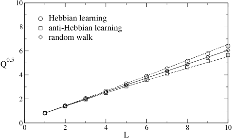
Abbildung 3.1: Length of the weight vectors in the steady state for $K=3$ and $N=1000$. Symbols denote results averaged over $1000$ simulations and lines show the first-order approximation given in (3.8) and (3.10).

In the case of the anti-Hebbian rule (2.7) A’s and B’s Tree Parity Machines learn the opposite of their own outputs. Therefore the weights are pulled away from the boundaries instead of being pushed towards $\pm L$. Here the first-order approximation of $Q_{i}$ is given by [22]

$$Q_{i}=\frac{L(L+1)}{3}-\frac{8L^{4}+16L^{3}-10L^{2}-18L+9}{15\sqrt{3\pi L(L+1)}}\frac{1}{\sqrt{N}}+\mathrm{O}\left(\frac{L^{4}}{N}\right)\,,$$ (3.10)

which asymptotically converges to

$$Q_{i}\sim\frac{L(L+1)}{3}\left(1-\frac{8}{5\sqrt{3\pi}}\frac{L}{\sqrt{N}}\right)$$ (3.11)

in the case $1\ll L\ll\sqrt{N}$. Hence applying the anti-Hebbian learning rule decreases the length of the weight vectors $\mathbf{w}_{i}$ until a steady state is reached. As before, $L/\sqrt{N}$ determines the size of this effect.

In contrast, the random walk rule (2.8) always uses a fixed set output. Here the weights stay uniformly distributed, as the random input values $x_{i,j}$ alone determine the direction of the movements. Consequently, the length of the weight vectors is always given by (3.6).

Figure 3.1 shows that the theoretical predictions are in good quantitative agreement with simulation results as long as $L^{2}$ is small compared to the system size $N$. The deviations for large $L$ are caused by higher-order terms which are ignored in (3.8) and (3.10).

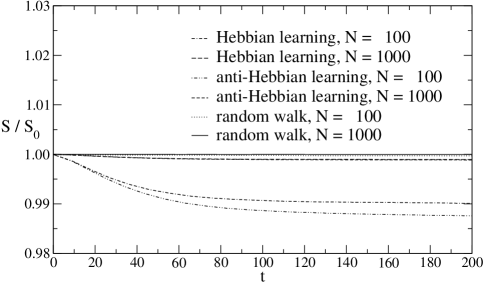
Abbildung 3.2: Time evolution of the weight distribution in the case of synchronization with $K=3$ and $L=5$, obtained in $100$ simulations consisting of $100$ pairs of Tree Parity Machines.

Of course, the change of the weight distribution is also directly visible in the relative entropy $S^{A}/S_{0}$ as shown in figure 3.2. While the weights are always uniformly distributed at the beginning of the synchronization process, so that $S^{A}=S_{0}$, only the random walk learning rule preserves this property. Otherwise $S^{A}$ decreases until the length of the weight vectors reaches its stationary state after a few steps. Therefore the transient has only little influence on the process of synchronization and one can assume a constant value of both $Q_{i}$ and $S^{A}$.

In the limit $N\rightarrow\infty$, however, a system using Hebbian or anti-Hebbian learning exhibits the same dynamics as observed in the case of the random walk rule for all system sizes. Consequently, there are two possibilities to determine the properties of neural synchronization without interfering finite-size effects. First, one can run simulations for the random walk learning rule and moderate system sizes. Second, the evolution of the probabilities $p_{a,b}^{i}$, which describe the distribution of the weights in two corresponding hidden units, can be calculated iteratively for $N\rightarrow\infty$. Both methods have been used in order to obtain the results presented in this thesis.

3.1.2 Attractive and repulsive steps

As the internal representation $(\sigma_{1},\sigma_{2},\dots,\sigma_{K})$ is not visible to other neural networks, two types of synchronization steps are possible:

• For $\tau^{A}=\sigma_{i}^{A}=\sigma_{i}^{B}=\tau^{B}$ the weights of both corresponding hidden units are moved in the same direction. As long as both weights, $w_{i,j}^{A}$ and $w_{i,j}^{B}$, stay in the range between $-L$ and $+L$, their distance $d_{i,j}=|w_{i,j}^{A}-w_{i,j}^{B}|$ remains unchanged. But if one of them hits the boundary at $\pm L$, it is reflected, so that $d_{i,j}$ decreases by one, until $d_{i,j}=0$ is reached. Therefore a sequence of these attractive steps leads to full synchronization eventually.

• If $\tau^{A}=\tau^{B}$, but $\sigma_{i}^{A}\not=\sigma_{i}^{B}$, only the weight vector of one hidden unit is changed. Two corresponding weights which have been already synchronized before, $w_{i,j}^{A}=w_{i,j}^{B}$, are separated by this movement, unless this is prevented by the boundary conditions. Consequently, this repulsive step reduces the correlations between corresponding weights and impedes the process of synchronization.

In all other situations the weights of the $i$-th hidden unit in A’s and B’s Tree Parity Machines are not modified at all.

In the limit $N\rightarrow\infty$ the effects of attractive and repulsive steps can be described by the following equations of motion for the probability distribution of the weights [17, 18, 19]. In attractive steps the weights perform an anisotropic diffusion

$$p_{a,b}^{i+}=\frac{1}{2}\left(p^{i}_{a+1,b+1}+p^{i}_{a-1,b-1}\right)$$ (3.12)

and move on the diagonals of a $(2L+1)\times(2L+1)$ square lattice. Repulsive steps, instead, are equal to normal diffusion steps

$$p_{a,b}^{i+}=\frac{1}{4}\left(p^{i}_{a+1,b}+p^{i}_{a-1,b}+p^{i}_{a,b+1}+p^{i}_{a,b-1}\right)$$ (3.13)

on the same lattice. However, one has to take the reflecting boundary conditions into account. Therefore (3.12) and (3.13) are only defined for $-L<a,b<+L$. Similar equations for the weights on the boundary can be found in appendix B.

Starting from the development of the variables $p_{a,b}$ one can calculate the change of the overlap in both types of steps. In general, the results

$$\Delta\rho_{\mathrm{a}}=\frac{3}{L(L+1)}\left(1-\sum_{j=-L}^{L}(2j+2)p_{L,j}+p_{L,L}\right)$$ (3.14)

for attractive steps and

$$\Delta\rho_{\mathrm{r}}=-\frac{3}{L(L+1)}\sum_{j=-L}^{L}\frac{j}{2}(p_{L,j}-p_{-L,j})$$ (3.15)

for repulsive steps are not only functions of the current overlap, but also depend explicitly on the probability distribution of the weights. That is why $\Delta\rho_{\mathrm{a}}(\rho)$ and $\Delta\rho_{\mathrm{r}}(\rho)$ are random variables, whose properties have to be determined in simulations of finite systems or iterative calculations for $N\rightarrow\infty$.

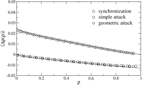
Abbildung 3.3: Effect of attractive (upper curve) and repulsive steps (lower curve) for $K=3$ and $L=10$. Symbols represent averages over $1000$ simulations using $N=100$ and the random walk learning rule. The line shows the corresponding result of $1000$ iterative calculations for synchronization in the limit $N\rightarrow\infty$.

Figure 3.3 shows that each attractive step increases the overlap on average. At the beginning of the synchronization it has its maximum effect [31],

$$\Delta\rho_{\mathrm{a}}(\rho=0)=\frac{12L}{(L+1)(2L+1)^{2}}\sim\frac{3}{L^{2}}\,,$$ (3.16)

as the weights are uncorrelated,

$$p_{a,b}(\rho=0)=\frac{1}{(2L+1)^{2}}\,.$$ (3.17)

But as soon as full synchronization is reached, an attractive step cannot increase the overlap further, so that $\Delta\rho_{\mathrm{a}}(\rho=1)=0$. Thus $\rho=1$ is a fixed point for a sequence of these steps.

In contrast, a repulsive step reduces a previously gained positive overlap on average. Its maximum effect [31],

$$\Delta\rho_{\mathrm{r}}(\rho=1)=-\frac{3}{(L+1)(2L+1)}\sim-\frac{3}{2L^{2}}\,,$$ (3.18)

is reached in the case of fully synchronized weights,

$$p_{a,b}(\rho=1)=\left\{\begin{array}[]{cl}(2L+1)^{-1}&\mbox{ for $a=b$ }\\ 0&\mbox{ for $a\not=b$ }\end{array}\right.\,.$$ (3.19)

But if the weights are uncorrelated, $\rho=0$, a repulsive step has no effect. Hence $\rho=0$ is a fixed point for a sequence of these steps.

It is clearly visible in figure 3.3 that the results obtained by simulations with the random walk learning rule and iterative calculations for $N\rightarrow\infty$ are in good quantitative agreement. This shows that both $\langle\Delta\rho_{\mathrm{a}}(\rho)\rangle$ and $\langle\Delta\rho_{\mathrm{r}}(\rho)\rangle$ are independent of the system size $N$. Additionally, the choice of the synchronization algorithm does not matter, which indicates a similar distribution of the weights for both unidirectional and bidirectional interaction. Consequently, the differences observed between learning and synchronization are caused by the probabilities of attractive and repulsive steps, but not their effects.

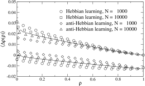
Abbildung 3.4: Effect of attractive (upper curves) and repulsive steps (lower curves) for different learning rules with $K=3$ and $L=10$. Symbols denote averages over $1000$ simulations, while the lines show the results of $1000$ iterative calculations.

However, the distribution of the weights is obviously altered by Hebbian and anti-Hebbian learning in finite systems, so that average change of the overlap in attractive and repulsive steps is different from the result for the random walk learning rule. This is clearly visible in figure 3.4. In the case of the Hebbian learning rule the effect of both types of steps is enhanced, but for anti-Hebbian learning it is reduced. It is even possible that an repulsive step has an attractive effect on average, if the overlap $\rho$ is small. This explains why one observes finite-size effects in the case of large $L/\sqrt{N}$ [16].

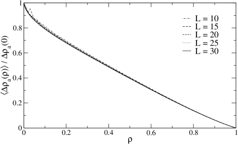
Abbildung 3.5: Scaling behavior of the average step size $\langle\Delta\rho_{\mathrm{a}}\rangle$ for attractive steps. These results were obtained in $1000$ iterative calculations for $K=3$ and $N\rightarrow\infty$.

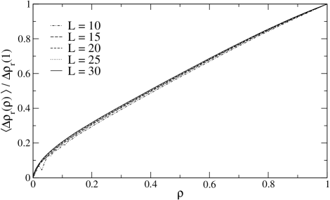
Abbildung 3.6: Scaling behavior of the average step size $\langle\Delta\rho_{\mathrm{r}}\rangle$ for repulsive steps. These results were obtained in $1000$ iterative calculations for $K=3$ and $N\rightarrow\infty$.

Using the equations (3.16) and (3.18) one can obtain the rescaled quantities $\langle\Delta\rho_{\mathrm{a}}(\rho)\rangle/\Delta\rho_{\mathrm{a}}(0)$ and $\langle\Delta\rho_{\mathrm{r}}(\rho)\rangle/\Delta\rho_{\mathrm{r}}(1)$. They become asymptotically independent of the synaptic depth $L$ in the limit $L\rightarrow\infty$ as shown in figure 3.5 and figure 3.6. Therefore these two scaling functions together with $\Delta\rho_{\mathrm{a}}(0)$ and $\Delta\rho_{\mathrm{r}}(1)$ are sufficient to describe the effect of attractive and repulsive steps [31].

3.2 Transition probabilities

While $\langle\Delta\rho_{\mathrm{a}}\rangle$ and $\langle\Delta\rho_{\mathrm{r}}\rangle$ are identical for synchronization and learning, the probabilities of attractive and repulsive steps depend on the type of interaction between the neural networks. Therefore these quantities are important for the differences between partners and attackers in neural cryptography.

A repulsive step can only occur if two corresponding hidden units have different $\sigma_{i}$. The probability for this event is given by the well-known generalization error [28]

$$\epsilon_{i}=\frac{1}{\pi}\arccos\rho_{i}$$ (3.20)

of the perceptron. However, disagreeing hidden units alone are not sufficient for a repulsive step, as the weights of all neural networks are only changed if $\tau^{A}=\tau^{B}$. Therefore the probability of a repulsive step is given by

$$P_{\mathrm{r}}=P(\sigma_{i}^{A}\not=\sigma_{i}^{B/E}|\tau^{A}=\tau^{B})\,,$$ (3.21)

after possible corrections of the output bits have been applied in the case of advanced learning algorithms. Similarly, one finds

$$P_{\mathrm{a}}=P(\tau^{A}=\sigma_{i}^{A}=\sigma_{i}^{B/E}|\tau^{A}=\tau^{B})$$ (3.22)

for the probability of attractive steps.

3.2.1 Simple attack

In the case of the simple attack, the outputs $\sigma_{i}^{E}$ of E’s Tree Parity Machine are not corrected before the application of the learning rule and the update of the weights occurs independent of $\tau^{E}$, as mutual interaction is not possible. Therefore a repulsive step in the $i$-th hidden unit occurs with probability [19]

$$P_{\mathrm{r}}^{E}=\epsilon_{i}\,.$$ (3.23)

But if two corresponding hidden units agree on their output $\sigma_{i}$, this does not always lead to an attractive step, because $\sigma_{i}=\tau$ is another necessary condition for an update of the weights. Thus the probability of an attractive step is given by [31]

$$P_{\mathrm{a}}^{E}=\frac{1}{2}(1-\epsilon_{i})$$ (3.24)

for $K>1$. In the special case $K=1$, however, $\sigma_{i}=\tau$ is always true, so that this type of steps occurs with double frequency: $P_{\mathrm{a}}^{E}=1-\epsilon_{i}$.

3.2.2 Synchronization

In contrast, mutual interaction is an integral part of bidirectional synchronization. When an odd number of hidden units disagrees on the output, $\tau^{A}\not=\tau^{B}$ signals that adjusting the weights would have a repulsive effect on at least one of the weight vectors. Therefore A and B skip this synchronization step.

But when an even number of hidden units disagrees on the output, the partners cannot detect repulsive steps by comparing $\tau^{A}$ and $\tau^{B}$. Additionally, identical internal representations in both networks are more likely than two or more different output bits $\sigma_{i}^{A}\not=\sigma_{i}^{B}$, if there are already some correlations between the Tree Parity Machines. Consequently, the weights are updated if $\tau^{A}=\tau^{B}$.

In the case of identical overlap in all $K$ hidden units, $\epsilon_{i}=\epsilon$, the probability of this event is given by

$$P_{\mathrm{u}}=P(\tau^{A}=\tau^{B})=\sum_{i=0}^{K/2}{K\choose 2i}(1-\epsilon)^{K-2i}\,\epsilon^{2i}\,.$$ (3.25)

Of course, only attractive steps are possible if two perceptrons learn from each other ($K=1$). But for synchronization of Tree Parity Machines with $K>1$, the probabilities of attractive and repulsive are given by:

$$P_{\mathrm{a}}^{B} = \frac{1}{2P_{\mathrm{u}}}\sum_{i=0}^{(K-1)/2}{K-1\choose 2i}(1-\epsilon)^{K-2i}\,\epsilon^{2i}\,,$$ (3.26)

$$P_{\mathrm{r}}^{B} = \frac{1}{P_{\mathrm{u}}}\sum_{i=1}^{K/2}{K-1\choose 2i-1}(1-\epsilon)^{K-2i}\,\epsilon^{2i}\,.$$ (3.27)

In the case of three hidden units ($K=3$), which is the usual choice for the neural key-exchange protocol, this leads to [19, 31]

$$P_{\mathrm{a}}^{B} = \frac{1}{2}\,\frac{(1-\epsilon)^{3}+(1-\epsilon)\epsilon^{2}}{(1-\epsilon)^{3}+3(1-\epsilon)\epsilon^{2}}\,,$$ (3.28)

$$P_{\mathrm{r}}^{B} = \frac{2(1-\epsilon)\epsilon^{2}}{(1-\epsilon)^{3}+3(1-\epsilon)\epsilon^{2}}\,.$$ (3.29)

Abbildung 3.7: Probability $P_{\mathrm{r}}^{B}(\rho)$ of repulsive steps for synchronization with mutual interaction under the condition $\tau^{A}=\tau^{B}$. The dotted line shows $P_{\mathrm{r}}^{E}(\rho)$ for a simple attack.

Figure 3.7 shows that repulsive steps occur more frequently in E’s Tree Parity Machine than in A’s or B’s for equal overlap $0<\rho<1$. That is why the partners A and B have a clear advantage over a simple attacker in neural cryptography. But this difference becomes smaller and smaller with increasing $K$. Consequently, a large number of hidden units is detrimental for the security of the neural key-exchange protocol against the simple attack.

3.2.3 Geometric attack

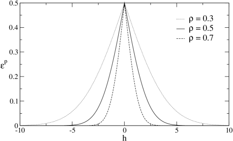
Abbildung 3.8: Prediction error $\epsilon_{i}^{\mathrm{p}}$ as a function of the local field $h_{i}^{E}$ for different values of the overlap $\rho_{i}^{AE}$ and $Q_{i}=1$.

However, E can do better than simple learning by taking the local field into account. Then the probability of $\sigma_{i}^{E}\not=\sigma_{i}^{A}$ is given by the prediction error [30]

$$\epsilon^{\mathrm{p}}_{i}=\frac{1}{2}\left[1-\mathrm{erf}\left(\frac{\rho_{i}}{\sqrt{2(1-\rho_{i}^{2})}}\frac{|h_{i}|}{\sqrt{Q_{i}}}\right)\right]$$ (3.30)

of the perceptron, which depends not only on the overlap $\rho_{i}$, but also on the absolute value $|h_{i}^{E}|$ of the local field. This quantity is a strictly decreasing function of $|h_{i}^{E}|$ as shown in figure 3.8. Therefore the geometric attack is often able to find the hidden unit with $\sigma_{i}^{E}\not=\sigma_{i}^{A}$ by searching for the minimum of $|h_{i}^{E}|$. If only the $i$-th hidden unit disagrees and all other have $\sigma_{j}^{E}=\sigma_{j}^{A}$, the probability for a successful correction of the internal representation by using the geometric attack is given by [22]

$$P_{\mathrm{g}}=\int_{0}^{\infty}\prod_{j\neq i}\left(\int_{h_{i}}^{\infty}\frac{2}{\sqrt{2\pi Q_{j}}}\frac{1-\epsilon^{\mathrm{p}}_{j}}{1-\epsilon_{j}}\,e^{-\frac{h_{j}^{2}}{2Q_{j}}}\,\mathrm{d}h_{j}\right)\frac{2}{\sqrt{2\pi Q_{i}}}\frac{\epsilon^{\mathrm{p}}_{i}}{\epsilon_{i}}\,e^{-\frac{h_{i}^{2}}{2Q_{i}}}\,\mathrm{d}h_{i}\,.$$ (3.31)

In the case of identical order parameters $Q=Q_{j}^{E}$ and $R=R_{j}^{AE}$ this equation can be easily extended to $k$ out of $K$ hidden units with different outputs $\sigma_{j}^{A}\not=\sigma_{j}^{E}$. Then the probability for successful correction of $\sigma_{i}^{E}\not=\sigma_{i}^{A}$ is given by

$$P_{k}^{+} = \int_{0}^{\infty}\left(\frac{2}{\sqrt{2\pi Q}}\right)^{K}\left(\int_{h_{i}}^{\infty}\frac{1-\epsilon^{\mathrm{p}}(h)}{1-\epsilon}\,e^{-\frac{h^{2}}{2Q}}\,\mathrm{d}h\right)^{K-k}$$ (3.32)

$$\times \left(\int_{h_{i}}^{\infty}\frac{\epsilon^{\mathrm{p}}(h)}{\epsilon}\,e^{-\frac{h^{2}}{2Q}}\,\mathrm{d}h\right)^{k-1}\frac{\epsilon^{\mathrm{p}}(h_{i})}{\epsilon}\,e^{-\frac{h_{i}^{2}}{2Q}}\,\mathrm{d}h_{i}\,.$$

Using a similar equation the probability for an erroneous correction of $\sigma_{i}^{E}=\sigma_{i}^{A}$ can be calculated, too:

$$P_{k}^{-} = \int_{0}^{\infty}\left(\frac{2}{\sqrt{2\pi Q}}\right)^{K}\left(\int_{h_{i}}^{\infty}\frac{1-\epsilon^{\mathrm{p}}(h)}{1-\epsilon}\,e^{-\frac{h^{2}}{2Q}}\,\mathrm{d}h\right)^{K-k-1}$$ (3.33)

$$\times \left(\int_{h_{i}}^{\infty}\frac{\epsilon^{\mathrm{p}}(h)}{\epsilon}\,e^{-\frac{h^{2}}{2Q}}\,\mathrm{d}h\right)^{k}\frac{1-\epsilon^{\mathrm{p}}(h_{i})}{1-\epsilon}\,e^{-\frac{h_{i}^{2}}{2Q}}\,\mathrm{d}h_{i}\,.$$

Taking all possible internal representations of A’s and E’s neural networks into account, the probability of repulsive steps consists of three parts in the case of the geometric attack.

• If the number of hidden units with $\sigma_{i}^{E}\not=\sigma_{i}^{A}$ is even, no geometric correction happens at all. This is similar to bidirectional synchronization, so that one finds

  $$P_{\mathrm{r,1}}^{E}=\sum_{i=1}^{K/2}{K-1\choose 2i-1}(1-\epsilon)^{K-2i}\,\epsilon^{2i}\,.$$ (3.34)

• It is possible that the hidden unit with the minimum $|h_{i}^{E}|$ has the same output as its counterpart in A’s Tree Parity Machine. Then the geometric correction increases the deviation of the internal representations. The second part of $P_{\mathrm{r}}^{E}$ takes this event into account:

  $$P_{\mathrm{r,2}}^{E}=\sum_{i=1}^{K/2}{K-1\choose 2i-1}P_{2i-1}^{-}\,(1-\epsilon)^{K-2i+1}\,\epsilon^{2i-1}\,.$$ (3.35)

• Similarly the geometric attack does not fix a deviation in the $i$-th hidden unit, if the output of another one is flipped instead. Indeed, this causes a repulsive step with probability

  $$P_{\mathrm{r,3}}^{E}=\sum_{i=0}^{(K-1)/2}{K-1\choose 2i}(1-P_{2i+1}^{+})(1-\epsilon)^{K-2i-1}\,\epsilon^{2i+1}\,.$$ (3.36)

Thus the probabilities of attractive and repulsive steps in the $i$-th hidden unit for $K>1$ and identical order parameters are given by

$$P_{\mathrm{a}}^{E} = \frac{1}{2}\left(1-\sum_{j=1}^{3}P_{\mathrm{r,j}}^{E}\right)\,,$$ (3.37)

$$P_{\mathrm{r}}^{E} = \sum_{j=1}^{3}P_{\mathrm{r,j}}^{E}\,.$$ (3.38)

In the case $K=1$, however, only attractive steps occur, because the algorithm of the geometric attack is then able to correct all deviations. And especially for $K=3$ one can calculate these probabilities using (3.31) instead of the general equations, which yields [22]

$$P_{\mathrm{a}}^{E} = \frac{1}{2}(1+2P_{\mathrm{g}})(1-\epsilon)^{2}\epsilon+\frac{1}{2}(1-\epsilon)^{3}$$ (3.39)

$$+ \frac{1}{2}(1-\epsilon)\epsilon^{2}+\frac{1}{6}\epsilon^{3}\,$$

$$P_{\mathrm{r}}^{E} = 2(1-P_{\mathrm{g}})(1-\epsilon)^{2}\epsilon+2(1-\epsilon)\epsilon^{2}+\frac{2}{3}\epsilon^{3}\,.$$ (3.40)

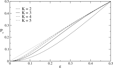
Abbildung 3.9: Probability of repulsive steps for an attacker using the geometric attack. The dotted line shows $P_{\mathrm{r}}$ for the simple attack.

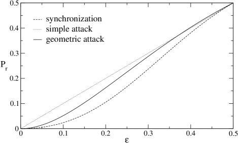
Abbildung 3.10: Probability of repulsive steps for Tree Parity Machines with $K=3$ hidden units and different types of interaction.

As shown in figure 3.9 $P_{\mathrm{r}}^{E}$ grows, if the number of hidden units is increased. It is even possible that the geometric attack performs worse than the simple attack at the beginning of the synchronization process ($\epsilon\approx 0.5$). While this behavior is similar to that observed in figure 3.7, $P_{\mathrm{r}}^{E}$ is still higher than $P_{\mathrm{r}}^{B}$ for identical $K$. Consequently, even this advanced algorithm for unidirectional learning has a disadvantage compared to bidirectional synchronization, which is clearly visible in figure 3.10.

3.3 Dynamics of the weights

In each attractive step corresponding weights of A’s and B’s Tree Parity Machines move in the same direction, which is chosen with equal probability in the case of the random walk learning rule. The same is true for Hebbian and anti-Hebbian learning in the limit $N\rightarrow\infty$ as shown in section 3.1.1. Of course, repulsive steps disturb this synchronization process. But for small overlap they have little effect, while they occur only seldom in the case of large $\rho$. That is why one can neglect repulsive steps in some situations and consequently describe neural synchronization as an ensemble of random walks with reflecting boundaries, driven by pairwise identical random signals [10, 9].

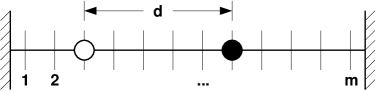
Abbildung 3.11: Random walks with reflecting boundaries.

This leads to a simple model for a pair of weights, which is shown in figure 3.11 [27]. Two random walks corresponding to $w_{i,j}^{A}$ and $w_{i,j}^{B}$ can move on a one-dimensional line with $m=2L+1$ sites. In each step a direction, either left or right, is chosen randomly. Then the random walkers move in this direction. If one of them hits the boundary, it is reflected, so that its own position remains unchanged. As this does not affect the other random walker, which moves towards the first one, the distance $d$ between them shrinks by $1$ at each reflection. Otherwise $d$ remains constant.

The most important quantity of this model is the synchronization time $T$ of the two random walkers, which is defined as the number of steps needed to reach $d=0$ starting with random initial positions. In order to calculate the mean value $\langle T\rangle$ and analyze the probability distribution $P(T=t)$, this process is divided into independent parts, each of them with constant distance $d$. Their duration $S_{d,z}$ is given by the time between two reflections. Of course, this quantity depends not only on the distance $d$, but also on the initial position $z=L+\mathrm{min}(w_{i,j}^{A},w_{i,j}^{B})+1$ of the left random walker.

3.3.1 Waiting time for a reflection

If the first move is to the right, a reflection only occurs for $z=m-d$. Otherwise, the synchronization process continues as if the initial position had been $z+1$. In this case the average number of steps with distance $d$ is given by $\langle S_{d,z+1}+1\rangle$. Similarly, if the two random walkers move to the left in the first step, this quantity is equal to $\langle S_{d,z-1}+1\rangle$. Averaging over both possibilities leads to the following difference equation [27]:

$$\langle S_{d,z}\rangle=\frac{1}{2}\langle S_{d,z-1}\rangle+\frac{1}{2}\langle S_{d,z+1}\rangle+1\,.$$ (3.41)

Reflections are only possible, if the current position $z$ is either $1$ or $m-d$. In both situations $d$ changes with probability $\frac{1}{2}$ in the next step, which is taken into account by using the boundary conditions

$$S_{d,0}=0\quad\mbox{and}\quad S_{d,m-d+1}=0\,.$$ (3.42)

As (3.41) is identical to the classical ruin problem [32], its solution is given by

$$\langle S_{d,z}\rangle=(m-d+1)z-z^{2}\,.$$ (3.43)

In order to calculate the standard deviation of the synchronization time an additional difference equation,

$$\langle S_{d,z}^{2}\rangle=\frac{1}{2}\langle(S_{d,z-1}+1)^{2}\rangle+\frac{1}{2}\langle(S_{d,z+1}+1)^{2}\rangle\,,$$ (3.44)

is necessary, which can be obtained in a similar manner as equation (3.41). Using both (3.43) and (3.44) leads to the relation [27]

$$\langle S_{d,z}^{2}\rangle-\langle S_{d,z}\rangle^{2} = \frac{\langle S_{d,z-1}^{2}\rangle-\langle S_{d,z-1}\rangle^{2}}{2}+\frac{\langle S_{d,z+1}^{2}\rangle-\langle S_{d,z+1}\rangle^{2}}{2}$$ (3.45)

$$+ (m-d+1-2z)^{2}$$

for the variance of $S_{d,z}$. Applying a Z-transformation finally yields the solution

$$\langle S_{d,z}^{2}\rangle-\langle S_{d,z}\rangle^{2}=\frac{(m-d+1-z)^{2}+z^{2}-2}{3}\,\langle S_{d,z}\rangle\,.$$ (3.46)

While the first two moments of $S_{d,z}$ are sufficient to calculate the mean value and the standard deviation of $T$, the probability distribution $P(S_{d,z}=t)$ must be known in order to further analyze $P(T=t)$. For that purpose a result known from the solution of the classical ruin problem [32] is used: The probability that a fair game ends with the ruin of one player in time step $t$ is given by

$$u(t)=\frac{1}{a}\sum_{k=1}^{a-1}\sin\left(\frac{k\pi z}{a}\right)\left[\sin\left(\frac{k\pi}{a}\right)+\sin\left(k\pi-\frac{k\pi}{a}\right)\right]\left[\cos\left(\frac{k\pi}{a}\right)\right]^{t-1}\,.$$ (3.47)

In the random walk model $a-1=m-d$ denotes the number of possible positions for two random walkers with distance $d$. And $u(t)$ is the probability distribution of the random variable $S_{d,z}$. As before, $z=L+\mathrm{min}(w_{i,j}^{A},w_{i,j}^{B})+1$ denotes the initial position of the left random walker.

3.3.2 Synchronization of two random walks

With these results one can determine the properties of the synchronization time $T_{d,z}$ for two random walks starting at position $z$ and distance $d$. After the first reflection at time $S_{d,z}$ one of the random walkers is located at the boundary. As the model is symmetric, both possibilities $z=1$ or $z=m-d$ are equal. Hence the second reflection takes place after $S_{d,z}+S_{d-1,1}$ steps and, consequently, the total synchronization time is given by

$$T_{d,z}=S_{d,z}+\sum_{j=1}^{d-1}S_{j,1}\,.$$ (3.48)

Using (3.43) leads to [27]

$$\langle T_{d,z}\rangle=(m-d+1)z-z^{2}+\,\frac{1}{2}(d-1)(2m-d)$$ (3.49)

for the expectation value of this random variable. In a similar manner one can calculate the variance of $T_{d,z}$, because the parts of the synchronization process are mutually independent.

Finally, one has to average over all possible initial conditions in order to determine the mean value and the standard deviation of the synchronization time $T$ for randomly chosen starting positions of the two random walkers [27]:

$$\langle T\rangle = \frac{2}{m^{2}}\sum_{d=1}^{m-1}\sum_{z=1}^{m-d}\langle T_{d,z}\rangle=\frac{(m-1)^{2}}{3}+\frac{m-1}{3m}\,,$$ (3.50)

$$\langle T^{2}\rangle = \frac{2}{m^{2}}\sum_{d=1}^{m-1}\sum_{z=1}^{m-d}\langle T_{d,z}^{2}\rangle$$ (3.51)

$$= \frac{17m^{5}-51m^{4}+65m^{3}-45m^{2}+8m+6}{90m}\,.$$

Abbildung 3.12: Synchronization time of two random walks as a function of the system size $m=2L+1$. Error bars denote the standard deviation observed in $1000$ simulations. The analytical solution (3.50) is plotted as dashed curve.

Thus the average number of attractive steps required to reach a synchronized state, which is shown in figure 3.12, increases nearly proportional to $m^{2}$. In particular for large system sizes $m$ the asymptotic behavior is given by

$$\langle T\rangle\sim\frac{1}{3}m^{2}\sim\frac{4}{3}L^{2}\,.$$ (3.52)

As shown later in section 3.4.1 this result is consistent with the scaling behavior $\langle t_{\mathrm{sync}}\rangle\propto L^{2}$ found in the case of neural synchronization [16].

In numerical simulations, both for random walks and neural networks, large fluctuations of the synchronization time are observed. The reason for this effect is that not only the mean value but also the standard deviation of $T$ [27],

$$\sigma_{T}=\sqrt{\frac{7m^{6}-11m^{5}-15m^{4}+55m^{3}-72m^{2}+46m-10}{90m^{2}}}\,,$$ (3.53)

increases with the extension $m$ of the random walks. A closer look at (3.52) and (3.53) reveals that $\sigma_{T}$ is asymptotically proportional to $\langle T\rangle$:

$$\sigma_{T}\sim\sqrt{\frac{7}{10}}\,\langle T\rangle\,.$$ (3.54)

Therefore the relative fluctuations $\sigma_{T}/\langle T\rangle$ are nearly independent of $m$ and not negligible. Consequently, one cannot assume a typical synchronization time, but has to take the full distribution $P(T=t)$ into account.

3.3.3 Probability distribution

As $T_{d,z}$ is the sum over $S_{i,j}$ for each distance $i$ from $d$ to $1$ according to (3.48), its probability distribution $\mathrm{P}(T_{d,z}=t)$ is a convolution of $d$ functions $u(t)$ defined in (3.47). The convolution of two different geometric sequences $b_{n}=b^{n}$ and $c_{n}=c^{n}$ is itself a linear combination of these sequences:

$$b_{n}\ast c_{n}=\sum_{j=1}^{n-1}b^{j}c^{n-j}=\frac{c}{b-c}\,b_{n}+\frac{b}{c-b}\,c_{n}\,.$$ (3.55)

Thus $\mathrm{P}(T_{d,z}=t)$ can be written as a sum over geometric sequences, too:

$$\mathrm{P}(T_{d,z}=t)=\sum_{a=m-d+1}^{m}\sum_{k=1}^{a-1}c^{d,z}_{a,k}\left[\cos\left(\frac{k\pi}{a}\right)\right]^{t-1}\,.$$ (3.56)

In order to obtain $\mathrm{P}(T=t)$ for random initial conditions, one has to average over all possible starting positions of both random walkers. But even this result

$$\mathrm{P}(T=t)=\frac{2}{m^{2}}\sum_{d=1}^{m-1}\sum_{z=1}^{m-d}\mathrm{P}(T_{d,z}=t)$$ (3.57)

can be written as a sum over a lot of geometric sequences:

$$\mathrm{P}(T=t)=\sum_{a=2}^{m}\sum_{k=1}^{a-1}c_{a,k}\left[\cos\left(\frac{k\pi}{a}\right)\right]^{t-1}\,.$$ (3.58)

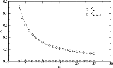
Abbildung 3.13: Value of the coefficients $c_{m,1}$ and $c_{m,m-1}$ as a function of $m$. The approximation given in (3.62) is shown as dashed curve.

For long times, however, only the terms with the largest absolute value of the coefficient $\cos(k\pi/a)$ are relevant, because the others decline exponentially faster. Hence one can neglect them in the limit $t\rightarrow\infty$, so that the asymptotic behavior of the probability distribution is given by

$$\mathrm{P}(T=t)\sim[c_{m,1}+(-1)^{t-1}c_{m,m-1}]\left[\cos\left(\frac{\pi}{m}\right)\right]^{t-1}\,.$$ (3.59)

The two coefficients $c_{m,1}$ and $c_{m,m-1}$ in this equation can be calculated using (3.55). This leads to the following result [27], which is shown in figure 3.13:

$$c_{m,1} \!\!=\!\! \frac{\sin^{2}(\pi/m)}{m^{2}m!}\sum_{d=1}^{m-1}\frac{2^{d+1}(m-d)!}{1-\delta_{d,1}\cos(\pi/m)}$$ (3.60)

$$\!\!\times\!\! \prod_{a=m-d+1}^{m-1}\sum_{k=1}^{a-1}\frac{\sin^{2}(k\pi/2)}{\cos(\pi/m)-\cos(k\pi/a)}\,\frac{\sin^{2}(k\pi/a)}{1-\delta_{a,m-d+1}\cos(k\pi/a)},$$

$$c_{m,m-1} \!\!=\!\! \frac{\sin^{2}(\pi/m)\cos^{2}(m\pi/2)}{m^{2}m!}\sum_{d=1}^{m-1}(-1)^{d-1}\frac{2^{d+1}(m-d)!}{1+\delta_{d,1}\cos(\pi/m)}$$ (3.61)

$$\!\!\times\!\! \prod_{a=m-d+1}^{m-1}\sum_{k=1}^{a-1}\frac{\sin^{2}(k\pi/2)}{\cos(\pi/m)+\cos(k\pi/a)}\,\frac{\sin^{2}(k\pi/a)}{1-\delta_{a,m-d+1}\cos(k\pi/a)}.$$

As the value of $c_{m,m-1}$ is given by an alternating sum, this coefficient is much smaller than $c_{m,1}$. Additionally, it is exactly zero for odd values of $m$ because of the factor $\cos^{2}(m\pi/2)$. The other coefficient $c_{m,1}$, however, can be approximated by [27]

$$c_{m,1}\approx 0.324\,m\left[1-\cos\left(\frac{\pi}{m}\right)\right]$$ (3.62)

for $m\gg 1$, which is clearly visible in figure 3.13, too.

Abbildung 3.14: Probability distribution $\mathrm{P}(T=t)$ of the synchronization time for $m=7$ ($L=3$). The numerical result is plotted as full curve. The dashed line denotes the asymptotic function defined in (3.63).

In the case of neural synchronization, $m=2L+1$ is always odd, so that $c_{m,m-1}=0$. Here $\mathrm{P}(T=t)$ asymptotically converges to a geometric probability distribution for long synchronization times:

$$\mathrm{P}(T=t)\sim c_{m,1}\left[\cos\left(\frac{\pi}{m}\right)\right]^{t-1}\,.$$ (3.63)

Figure 3.14 shows that this analytical solution describes $P(T=t)$ well, except for some deviations at the beginning of the synchronization process. But for small values of $t$ one can use the equations of motion for $p_{a,b}$ in order to calculate $P(T=t)$ iteratively.

3.3.4 Extreme order statistics

In this section the model is extended to $N$ independent pairs of random walks driven by identical random noise. This corresponds to two hidden units with $N$ weights, which start uncorrelated and reach full synchronization after $T_{N}$ attractive steps.

Although $\langle T\rangle$ is the mean value of the synchronization time for a pair of weights, $w_{i,j}^{A}$ and $w_{i,j}^{B}$, it is not equal to $\langle T_{N}\rangle$. The reason is that the weight vectors have to be completely identical in the case of full synchronization. Therefore $T_{N}$ is the maximum value of $T$ observed in $N$ independent samples corresponding to the different weights of a hidden unit.

As the distribution function $\mathrm{P}(T\leq t)$ is known, the probability distribution of $T_{N}$ is given by

$$\mathrm{P}(T_{N}\leq t)=\mathrm{P}(T\leq t)^{N}\,.$$ (3.64)

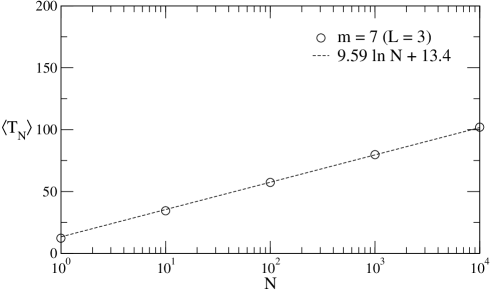
Abbildung 3.15: Average synchronization time $\langle T_{N}\rangle$ as a function of $N$ for $m=7$ ($L=3$). Results of the numerical calculation using (3.64) are represented by circles. The dashed line shows the expectation value of $T_{N}$ calculated in (3.69).

Hence one can calculate the average value $\langle T_{N}\rangle$ using the numerically computed distribution $\mathrm{P}(T_{N}\leq t)$. The result, which is shown in figure 3.15, indicates that $\langle T_{N}\rangle$ increases logarithmically with the number of pairs of random walkers:

$$\langle T_{N}\rangle-\langle T\rangle\propto\ln N\,.$$ (3.65)

For large $N$ only the asymptotic behavior of $\mathrm{P}(T\leq t)$ is relevant for the distribution of $T_{N}$. The exponential decay of $\mathrm{P}(T=t)$ according to (3.59) yields a Gumbel distribution for $\mathrm{P}(T_{N}\leq t)$ [33],

$$G(t)=\exp\left(-e^{\frac{t_{\mathrm{a}}-t}{t_{\mathrm{b}}}}\right)\,,$$ (3.66)

for $N\gg m$ with the parameters

$$t_{\mathrm{a}}=t_{\mathrm{b}}\ln\frac{Nc_{m,1}}{1-\cos(\pi/m)}\quad\mbox{and}\quad t_{\mathrm{b}}=-\frac{1}{\ln\cos(\pi/m)}\,.$$ (3.67)

Substituting (3.67) into (3.66) yields [27]

$$\mathrm{P}(T_{N}\leq t)=\exp\left(-\frac{Nc_{m,1}\cos^{t}(\pi/m)}{1-\cos(\pi/m)}\right)$$ (3.68)

as the distribution function for the total synchronization time of $N$ pairs of random walks ($N\gg m$). The expectation value of this probability distribution is given by [33]

$$\langle T_{N}\rangle=t_{\mathrm{a}}+t_{\mathrm{b}}\gamma=-\frac{1}{\ln\cos(\pi/m)}\left(\gamma+\ln N+\ln\frac{c_{m,1}}{1-\cos(\pi/m)}\right)\,.$$ (3.69)

Here $\gamma$ denotes the Euler-Mascheroni constant. For $N\gg m\gg 1$ the asymptotic behavior of the synchronization time is given by

$$\langle T_{N}\rangle\sim\frac{2}{\pi^{2}}\,m^{2}\left(\gamma+\ln N+\ln\frac{2m^{2}\,c_{m,1}}{\pi^{2}}\right)\,.$$ (3.70)

Using (3.62) finally leads to the result [27]

$$\langle T_{N}\rangle\approx\frac{2}{\pi^{2}}\,m^{2}\left(\ln N+\ln(0.577\,m)\right)\,,$$ (3.71)

which shows that $\langle T_{N}\rangle$ increases proportional to $m^{2}\ln N$.

Of course, neural synchronization is somewhat more complex than this model using random walks driven by pairwise identical noise. Because of the structure of the learning rules the weights are not changed in each step. Including these idle steps certainly increases the synchronization time $t_{\mathrm{sync}}$. Additionally, repulsive steps destroying synchronization are possible, too. Nevertheless, a similar scaling law $\langle t_{\mathrm{sync}}\rangle\propto L^{2}\ln N$ can be observed for the synchronization of two Tree Parity Machines as long as repulsive effects have only little influence on the dynamics of the system.

3.4 Random walk of the overlap

The most important order parameter of the synchronization process is the overlap between the weight vectors of the participating neural networks. The results of section 3.1 and section 3.2 indicate that its change over time can be described by a random walk with position dependent step sizes, $\langle\Delta\rho_{\mathrm{a}}\rangle$, $\langle\Delta\rho_{\mathrm{r}}\rangle$, and transition probabilities, $P_{\mathrm{a}}$, $P_{\mathrm{r}}$ [31]. Of course, only the transition probabilities are exact functions of $\rho$, while the step sizes fluctuate randomly around their average values. Consequently, this model is not suitable for quantitative predictions, but nevertheless one can determine important properties regarding the qualitative behavior of the system. For this purpose, the average change of the overlap

$$\langle\Delta\rho\rangle=P_{\mathrm{a}}(\rho)\langle\Delta\rho_{\mathrm{a}}(\rho)\rangle+P_{\mathrm{r}}(\rho)\langle\Delta\rho_{\mathrm{r}}(\rho)\rangle$$ (3.72)

in one synchronization step as a function of $\rho$ is especially useful.

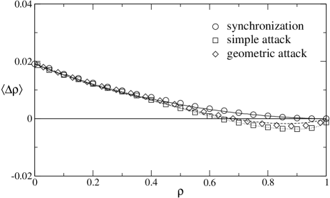
Abbildung 3.16: Average change of the overlap for $K=3$, $L=5$, and random walk learning rule. Symbols denote results obtained from $1000$ simulations, while the lines have been calculated using (3.72).

Figure 3.16 clearly shows the difference between synchronization and learning for $K=3$. In the case of bidirectional interaction, $\langle\Delta\rho\rangle$ is always positive until the process reaches the absorbing state at $\rho=1$. But for unidirectional interaction, there is a fixed point at $\rho_{\mathrm{f}}<1$. That is why a further increase of the overlap is only possible by fluctuations. Consequently, there are two different types of dynamics, which play a role in the process of synchronization.

3.4.1 Synchronization on average

If $\langle\Delta\rho\rangle$ is always positive for $\rho<1$, each update of the weights has an attractive effect on average. In this case repulsive steps delay the process of synchronization, but the dynamics is dominated by the effect of attractive steps. Therefore it is similar to that of random walks discussed in section 3.3.

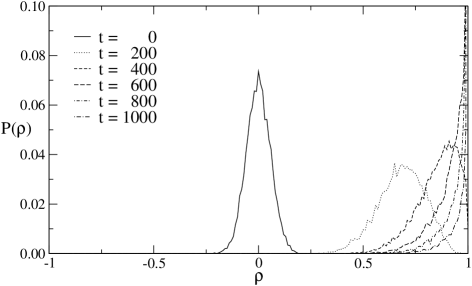
Abbildung 3.17: Distribution of the overlap in different time steps. These results were obtained in $100$ simulations for synchronization with $K=3$, $L=5$, $N=100$, and random walk learning rule.

As shown in figure 3.17 the distribution of the overlap gets closer to the absorbing state at $\rho=1$ in each time step. And the velocity of this process is determined by $\langle\Delta\rho\rangle$. That is why $\rho$ increases fast at the beginning of the synchronization, but more slowly towards the end.

However, the average change of the overlap depends on the synaptic depth $L$, too. While the transition probabilities $P_{\mathrm{a}}$ and $P_{\mathrm{r}}$ are unaffected by a change of $L$, the step sizes $\langle\Delta\rho_{\mathrm{a}}\rangle$ and $\langle\Delta\rho_{\mathrm{r}}\rangle$ shrink proportional to $L^{-2}$ according to (3.16) and (3.18). Hence $\langle\Delta\rho\rangle$ also decreases proportional to $L^{-2}$ so that a large synaptic depth slows down the dynamics. That is why one expects

$$\langle t_{\mathrm{sync}}\rangle\propto\frac{1}{\langle\Delta\rho\rangle}\propto L^{2}$$ (3.73)

for the scaling of the synchronization time.

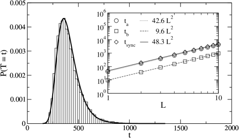
Abbildung 3.18: Probability distribution of the synchronization time for two Tree Parity Machines with $K=3$, $L=3$, $N=1000$, and random walk learning rule. The histogram shows the relative frequency of occurrence observed in $10\,000$ simulations and the thick curve represents a fit of the Gumbel distribution. Fit parameters for different values of $L$ are shown in the inset.

In fact, the probability $P(t_{\mathrm{sync}}\leq t)$ to achieve identical weight vectors in A’s and B’s neural networks in at most $t$ steps is described well by a Gumbel distribution (3.66):

$$P_{\mathrm{sync}}^{B}(t)=\exp\left(-e^{\frac{t_{\mathrm{a}}-t}{t_{\mathrm{b}}}}\right)\,.$$ (3.74)

Similar to the model in section 3.3 the parameters $t_{\mathrm{a}}$ and $t_{\mathrm{b}}$ increase both proportional to $L^{2}$, which is clearly visible in figure 3.18. Consequently, the average synchronization time scales like $\langle t_{\mathrm{sync}}\rangle\propto L^{2}\ln N$, in agreement with (3.71).

Additionally, figure 3.17 indicates that large fluctuations of the overlap can be observed during the process of neural synchronization. For $t=0$ the width of the distribution is due to the finite number of weights and vanishes in the limit $N\rightarrow\infty$. But later fluctuations are mainly amplified by the interplay of discrete attractive and repulsive steps. This effect cannot be avoided by increasing $N$, because this does not change the step sizes. Therefore the order parameter $\rho$ is not a self-averaging quantity [34]: one cannot replace $\rho$ by $\langle\rho\rangle$ in the equations of motion in order to calculate the time evolution of the overlap analytically. Instead, the whole probability distribution of the weights has to be taken into account.

3.4.2 Synchronization by fluctuations

If there is a fixed point at $\rho_{\mathrm{f}}<1$, then the dynamics of neural synchronization changes drastically. As long as $\rho<\rho_{\mathrm{f}}$ the overlap increases on average. But then a quasi-stationary state is reached. Further synchronization is only possible by fluctuations, which are caused by the discrete nature of attractive and repulsive steps.

Abbildung 3.19: Distribution of the overlap in different time steps. These results were obtained in $100$ simulations for the geometric attack with $K=3$, $L=5$, $N=100$, and random walk learning rule.

Figure 3.19 shows both the initial transient and the quasi-stationary state. The latter can be described by a normal distribution with average value $\rho_{\mathrm{f}}$ and a standard deviation $\sigma_{\mathrm{f}}$.

In order to determine the scaling of the fluctuations, a linear approximation of $\langle\Delta\rho(\rho)\rangle$ is used as a simple model [31],

$$\Delta\rho(t)=-\alpha_{\mathrm{f}}(\rho(t)-\rho_{\mathrm{f}})+\beta_{\mathrm{f}}\xi(t)\,,$$ (3.75)

without taking the boundary conditions into account. Here the $\xi(t)$ are random numbers with zero mean and unit variance. The two parameters are defined as

$$\alpha_{\mathrm{f}} = -\left.\frac{\mathrm{d}}{\mathrm{d}\rho}\langle\Delta\rho(\rho)\rangle\right|_{\rho=\rho_{\mathrm{f}}}\,,$$ (3.76)

$$\beta_{\mathrm{f}} = \sqrt{\langle(\Delta\rho(\rho_{\mathrm{f}}))^{2}\rangle}\,.$$ (3.77)

In this model, the solution of (3.75),

$$\rho(t+1)-\rho_{\mathrm{f}}=\beta_{\mathrm{f}}\sum_{i=0}^{t}(1-\alpha_{\mathrm{f}})^{t-i}\xi(i)\,,$$ (3.78)

describes the time evolution of the overlap. Here the initial condition $\rho(0)=\rho_{\mathrm{f}}$ was assumed, which is admittedly irrelevant in the limit $t\rightarrow\infty$. Calculating the variance of the overlap in the stationary state yields [31]

$$\sigma_{\mathrm{f}}^{2}=\beta_{\mathrm{f}}^{2}\sum_{t=0}^{\infty}(1-\alpha_{\mathrm{f}})^{2t}=\frac{\beta_{\mathrm{f}}^{2}}{2\alpha_{\mathrm{f}}-\alpha_{\mathrm{f}}^{2}}\,.$$ (3.79)

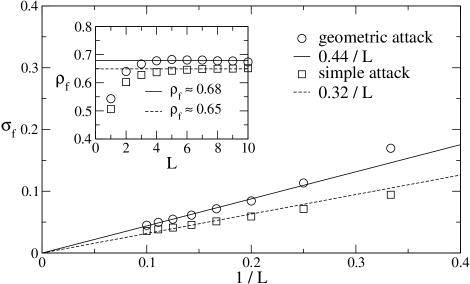
Abbildung 3.20: Standard deviation of $\rho$ at the fixed point for $K=3$, $N=1000$, random walk learning rule, and unidirectional synchronization, averaged over $10\,000$ simulations. The inset shows the position of the fixed point.

As the step sizes of the random walk in $\rho$-space decrease proportional to $L^{-2}$ for $L\gg 1$ according to (3.16) and (3.18), this is also the scaling behavior of the parameters $\alpha_{\mathrm{f}}$ and $\beta_{\mathrm{f}}$. Thus one finds

$$\sigma_{\mathrm{f}}\propto\frac{1}{L}$$ (3.80)

for larger values of the synaptic depth. Although this simple model does not include the more complex features of $\langle\Delta\rho(\rho)\rangle$, its scaling behavior is clearly reproduced in figure 3.20. Deviations for small values of $L$ are caused by finite-size effects.

Consequently, E is unable to synchronize with A and B in the limit $L\rightarrow\infty$, even if she uses the geometric attack. This is also true for any other algorithm resulting in a dynamics of the overlap, which has a fixed point at $\rho_{\mathrm{f}}<1$.

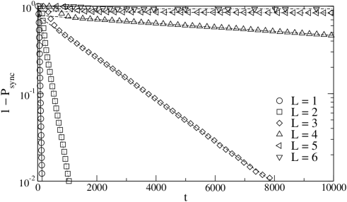
Abbildung 3.21: Probability distribution of $t_{\mathrm{sync}}$ for $K=3$, $N=1000$, random walk learning rule, and geometric attack. Symbols denote results averaged over $1000$ simulations and the lines show fits with (3.81).

For finite synaptic depth, however, the attacker has a chance of getting beyond the fixed point at $\rho_{\mathrm{f}}$ by fluctuations. The probability that this event occurs in any given step is independent of $t$, once the quasi-stationary state has been reached. Thus $P^{E}_{\mathrm{sync}}(t)$ is not given by a Gumbel distribution (3.66), but described well for $t\gg t_{0}$ by an exponential distribution,

$$P^{E}_{\mathrm{sync}}(t)=1-e^{-\frac{t-t_{0}}{t_{\mathrm{f}}}}\,,$$ (3.81)

with time constant $t_{\mathrm{f}}$. This is clearly visible in figure 3.21. Because of $t_{\mathrm{f}}\gg t_{0}$ one needs

$$\langle t_{\mathrm{sync}}\rangle\approx\left\{\begin{array}[]{cl}t_{\mathrm{f}}\,e^{t_{0}/t_{\mathrm{f}}}&\mbox{ for $t_{0}<0$}\\ t_{\mathrm{f}}+t_{0}&\mbox{ for $t_{0}\geq 0$}\end{array}\right\}\approx t_{\mathrm{f}}$$ (3.82)

steps on average to reach $\rho=1$ using unidirectional learning.

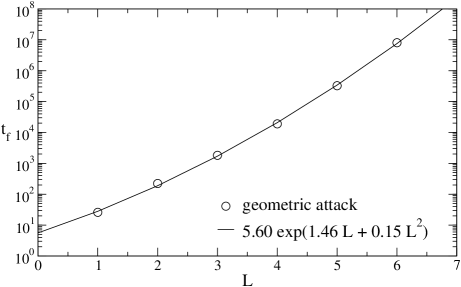
Abbildung 3.22: Time constant $t_{\mathrm{f}}$ for synchronization by fluctuations. Symbols denote results obtained in $1000$ simulations of the geometric attack for $K=3$, $N=1000$, and random walk learning rule. The line shows a fit with (3.85).

In the simplified model [31] with linear $\langle\Delta\rho(\rho)\rangle$ the mean time needed to achieve full synchronization starting at the fixed point is given by

$$t_{\mathrm{f}}\approx\frac{1}{P(\rho=1)}=\sqrt{2\pi}\sigma_{\mathrm{f}}e^{\frac{(1-\rho_{\mathrm{f}})^{2}}{2\sigma_{\mathrm{f}}^{2}}}$$ (3.83)

as long as the fluctuations are small. If $\sigma_{\mathrm{f}}\ll 1-\rho_{\mathrm{f}}$, the assumption is reasonable, that the distribution of $\rho$ is not influenced by the presence of the absorbing state at $\rho=1$. Hence one expects

$$t_{\mathrm{f}}\propto e^{cL^{2}}$$ (3.84)

for the scaling of the time constant, as $\sigma_{\mathrm{f}}$ changes proportional to $L^{-1}$, while $\rho_{\mathrm{f}}$ stays nearly constant. And figure 3.22 shows that indeed $t_{\mathrm{f}}$ grows exponentially with increasing synaptic depth:

$$t_{\mathrm{f}}\propto e^{c_{1}L+c_{2}L^{2}}\,.$$ (3.85)

Thus the partners A and B can control the complexity of attacks on the neural key-exchange protocol by choosing $L$. Or if E’s effort stays constant, her success probability drops exponentially with increasing synaptic depth. As shown in chapter 4, this effect can be observed in the case of the geometric attack [16] and even for advanced methods [23, 22].

3.5 Synchronization time

As shown before the scaling of the average synchronization time $\langle t_{\mathrm{sync}}\rangle$ with regard to the synaptic depth $L$ depends on the function $\langle\Delta\rho(\rho)\rangle$ which is different for bidirectional and unidirectional interaction. However, one has to consider two other parameters. The probability of repulsive steps $P_{\mathrm{r}}$ depends not only on the interaction, but also on the number of hidden units. Therefore one can switch between synchronization on average and synchronization by fluctuations by changing $K$, which is the topic of section 3.5.1. Additionally, the chosen learning rule influences the step sizes of attractive and repulsive steps. Section 3.5.2 shows that this affects $\langle\Delta\rho(\rho)\rangle$ and consequently the average synchronization time $\langle t_{\mathrm{sync}}\rangle$, too.

3.5.1 Number of hidden units

As long as $K\leq 3$, A and B are able to synchronize on average. In this case $\langle t_{\mathrm{sync}}\rangle$ increases proportional to $L^{2}$. In contrast, E can only synchronize by fluctuations as soon as $K>1$, so that for her $\langle t_{\mathrm{sync}}\rangle$ grows exponentially with the synaptic depth $L$. Consequently, A and B can reach any desired level of security by choosing a suitable value for $L$.

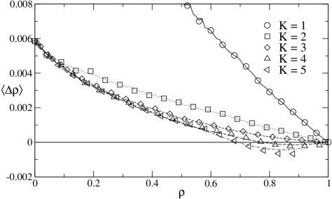
Abbildung 3.23: Average change of the overlap for $L=10$, $N=1000$, random walk learning rule, and bidirectional synchronization. Symbols denote results obtained from $100$ simulations, while the lines have been calculated using (3.72).

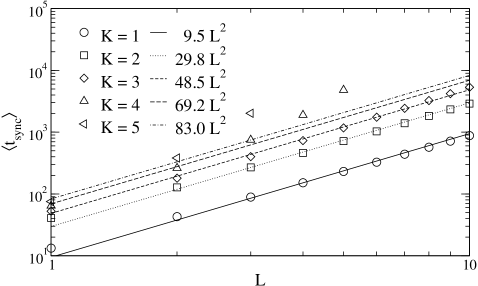
Abbildung 3.24: Synchronization time for bidirectional interaction, $N=1000$, and random walk learning rule. Symbols denote results averaged over $10\,000$ simulations and the lines represent fits of the model $\langle t_{\mathrm{sync}}\rangle\propto L^{2}$.

However, this is not true for $K>3$. As shown in figure 3.23, a fixed point at $\rho_{\mathrm{f}}<1$ appears in the case of bidirectional synchronization, too. Therefore (3.73) is not valid any more and $\langle t_{\mathrm{sync}}\rangle$ now increases exponentially with $L$. This is clearly visible in figure 3.24. Consequently, Tree Parity Machines with four and more hidden units cannot be used in the neural key-exchange protocol, except if the synaptic depth is very small.

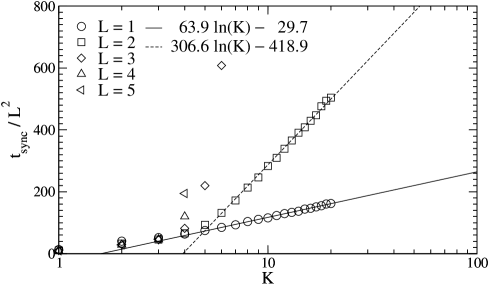
Abbildung 3.25: Synchronization time for bidirectional interaction, $N=1000$, and random walk learning rule, averaged over $1000$ simulations.

Figure 3.25 shows the transition between the two mechanisms of synchronization clearly. As long as $K\leq 3$ the scaling law $\langle t_{\mathrm{sync}}\rangle\propto L^{2}$ is valid, so that the constant of proportionality $\langle t_{\mathrm{sync}}\rangle/L^{2}$ is independent of the number of hidden units. Additionally, it increases proportional to $\ln KN$, as the total number of weights in a Tree Parity Machine is given by $KN$.

In contrast, $\langle t_{\mathrm{sync}}\rangle\propto L^{2}$ is not valid for $K>3$. In this case $\langle t_{\mathrm{sync}}\rangle/L^{2}$ still increases proportional to $\ln KN$, but the steepness of the curve depends on the synaptic depth, as the fluctuations of the overlap decrease proportional to $L^{-1}$. Consequently, there are two sets of parameters, which allow for synchronization using bidirectional interaction in a reasonable number of steps: the absorbing state $\rho=1$ is reached on average for $K\leq 3$, whereas large enough fluctuations drive the process of synchronization in the case of $L\leq 3$ and $K\geq 4$. Otherwise, a huge number of steps is needed to achieve full synchronization.

3.5.2 Learning rules

Although the qualitative properties of neural synchronization are independent of the chosen learning rule, one can observe quantitative deviations for Hebbian and anti-Hebbian learning in terms of finite-size effects. Of course, these disappear in the limit $L/\sqrt{N}\rightarrow 0$.

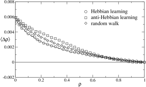
Abbildung 3.26: Average change of the overlap for $K=3$, $L=10$, $N=1000$, and bidirectional synchronization. Symbols denote results obtained from $100$ simulations, while the lines have been calculated using (3.72).

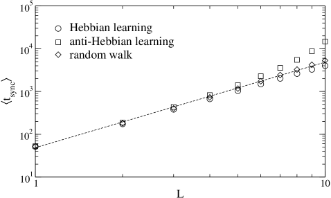
Abbildung 3.27: Synchronization time for bidirectional interaction and $K=3$. Symbols denote results averaged over $10\,000$ simulations and the line shows the corresponding fit from figure 3.24 for the random walk learning rule.

As shown in section 3.1 Hebbian learning enhances the effects of both repulsive and attractive steps. This results in a decrease of $\langle\Delta\rho\rangle$ for small overlap, where a lot of repulsive steps occur. But if A’s and B’s Tree Parity Machines are nearly synchronized, attractive steps prevail, so that the average change of the overlap is increased compared to the random walk learning rule. This is clearly visible in figure 3.26. Of course, anti-Hebbian learning reduces both step sizes and one observes the opposite effect.

However, the average synchronization time $\langle t_{\mathrm{sync}}\rangle$ is mainly influenced by the transition from $\rho\approx 1$ to $\rho=1$, which is the slowest part of the synchronization process. Therefore Hebbian learning decreases the average number of steps needed to achieve full synchronization. This effect is clearly visible in figure 3.27.

In contrast, anti-Hebbian learning increases $\langle t_{\mathrm{sync}}\rangle$. Here finite-size effects cause problems for bidirectional synchronization, because one can even observe $\langle\Delta\rho\rangle<0$ for $K=3$, if $L/\sqrt{N}$ is just sufficiently large. Then the synchronization time increases faster than $L^{2}$. Consequently, this learning rule is only usable in large systems, where finite-size effects are small and the observed behavior is similar to that of the random walk learning rule.

Kapitel 4 Security of neural cryptography

The security of the neural key-exchange protocol is based on the phenomenon analyzed in chapter 2: two Tree Parity Machines interacting with each other synchronize much faster than a third neural network trained using their inputs and outputs as examples. In fact, the effort of the partners grows only polynomially with increasing synaptic depth, while the complexity of an attack scales exponentially with $L$.

However, neural synchronization is a stochastic process driven by random attractive and repulsive forces [19]. Therefore A and B are not always faster than E, but there is a small probability $P_{E}$ that an attacker is successful before the partners have finished the key exchange. Because of the different dynamics $P_{E}$ drops exponentially with increasing $L$, so that the system is secure in the limit $L\rightarrow\infty$ [16]. And in practise, one can reach any desired level of security by just increasing $L$, while the effort of generating a key only grows moderately [22].

Although this mechanism works perfectly, if the parameters of the protocol are chosen correctly, other values can lead to an insecure key exchange [21]. Therefore it is necessary to determine the scaling of $P_{E}$ for different configurations and all known attack methods. By doing so, one can form an estimate regarding the minimum synaptic depth needed for some practical applications, too.

While $P_{E}$ directly shows whether neural cryptography is secure, it does not reveal the cause of this observation. For that purpose, it is useful to analyze the mutual information $I$ gained by partners and attackers during the process of synchronization. Even though all participants receive the same messages, A and B can select the most useful ones for adjusting the weights. That is why they learn more about each other than E, who is only listening. Consequently, bidirectional interaction gives an advantage to the partners, which cannot be exploited by a passive attacker.

Of course, E could try other methods instead of learning by listening. Especially in the case of a brute-force attack, security depends on the number of possible keys, which can be generated by the neural key-exchange protocol. Therefore it is important to analyze the scaling of this quantity, too.

4.1 Success probability

Attacks which are based on learning by listening have in common that the opponent E tries to synchronize one or more Tree Parity Machines with A’s and B’s neural networks. Of course, after the partners have reached identical weight vectors, they stop the process of synchronization, so that the number of available examples for the attack is limited. Therefore E’s online learning is only successful, if she discovers the key before A and B finish the key exchange.

As synchronization of neural networks is a stochastic process, there is a small probability that E synchronizes faster with A than B. In actual fact, one could use this quantity directly to describe the security of the key-exchange protocol. However, the partners may not detect full synchronization immediately, so that E is even successful, if she achieves her goal shortly afterwards. Therefore $P_{E}$ is defined as the probability that the attacker knows 98 per cent of the weights at synchronization time. Additionally, this definition reduces fluctuations in the simulations, which are employed to determine $P_{E}$ [16].

4.1.1 Attacks using a single neural network

For both the simple attack and the geometric attack E only needs one Tree Parity Machine. So the complexity of these methods is small. But as already shown in section 3.4.2 E can only synchronize by fluctuations if $K>1$, while the partners synchronize on average as long as $K\leq 3$. That is why $t_{\mathrm{sync}}^{E}$ is usually much larger than $t_{\mathrm{sync}}^{B}$ for $K=2$ and $K=3$. In fact, the probability of $t_{\mathrm{sync}}^{E}\leq t_{\mathrm{sync}}^{B}$ in this case is given by

$$P(t_{\mathrm{sync}}^{E}\leq t_{\mathrm{sync}}^{B})=\int_{t=0}^{\infty}P_{\mathrm{sync}}^{E}(t)\,\frac{\mathrm{d}}{\mathrm{d}t}P_{\mathrm{sync}}^{B}(t)\,\mathrm{d}t$$ (4.1)

under the assumption that the two synchronization times are uncorrelated random variables. In this equation $P_{\mathrm{sync}}^{B}(t)$ and $P_{\mathrm{sync}}^{E}(t)$ are the cumulative probability distributions of the synchronization time defined in (3.74) and (3.81), respectively.

In order to approximate this probability one has to look especially at the fluctuations of the synchronization times $t_{\mathrm{sync}}^{B}$ and $t_{\mathrm{sync}}^{E}$. The width of the Gumbel distribution,

$$\sqrt{\langle(t_{\mathrm{sync}}^{B})^{2}\rangle-\langle t_{\mathrm{sync}}^{B}\rangle^{2}}=\frac{\pi}{\sqrt{6}}\,t_{\mathrm{b}}\,,$$ (4.2)

for A and B is much smaller than the standard deviation of the exponential distribution,

$$\sqrt{\langle(t_{\mathrm{sync}}^{E})^{2}\rangle-\langle t_{\mathrm{sync}}^{E}\rangle^{2}}=t_{\mathrm{f}}\,,$$ (4.3)

for E because of $t_{\mathrm{f}}\gg t_{\mathrm{b}}$. Therefore one can approximate $P_{\mathrm{sync}}^{B}(t)$ in integral (4.1) by $\Theta(t-\langle t_{\mathrm{sync}}^{B}\rangle)$, which leads to

$$P(t_{\mathrm{sync}}^{E}\leq t_{\mathrm{sync}}^{B})\approx 1-\exp\left(-\frac{\langle t_{\mathrm{sync}}^{B}\rangle}{\langle t_{\mathrm{sync}}^{E}\rangle}\right)\,.$$ (4.4)

Hence the success probability of an attack depends on the ratio of both average synchronization times,

$$\frac{\langle t_{\mathrm{sync}}^{B}\rangle}{\langle t_{\mathrm{sync}}^{E}\rangle}\propto\frac{L^{2}}{e^{c_{1}L+c_{2}L^{2}}}\,,$$ (4.5)

which are functions of the synaptic depth $L$ according to (3.73) and (3.85). Consequently, $L$ is the most important parameter for the security of the neural key-exchange protocol.

In the case of $L\gg 1$ the ratio $\langle t_{\mathrm{sync}}^{B}\rangle/\langle t_{\mathrm{sync}}^{E}\rangle$ becomes very small, so that a further approximation of (4.4) is possible. This yields the result

$$P(t_{\mathrm{sync}}^{E}\leq t_{\mathrm{sync}}^{B})\propto L^{2}e^{-c_{1}L}e^{-c_{2}L^{2}}\,,$$ (4.6)

which describes the asymptotic behavior of the success probability: if A and B increase the synaptic depth of their Tree Parity Machines, the success probability of an attack drops exponentially [16]. Thus the partners can achieve any desired level of security by changing $L$.

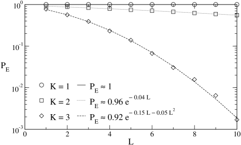
Abbildung 4.1: Success probability of the geometric attack as a function of $L$. Symbols denote results obtained in $10\,000$ simulations with $N=1000$ and random walk learning rule, while the lines represent fit results for model (4.7).

Although $P_{E}$ is not exactly identical to $P(t_{\mathrm{sync}}^{E}\leq t_{\mathrm{sync}}^{B})$ because of its definition, it has the expected scaling behavior,

$$P_{E}\propto e^{-y_{1}L-y_{2}L^{2}}\,,$$ (4.7)

which is clearly visible in figure 4.1. However, the coefficients $y_{1}$ and $y_{2}$ are different from $c_{1}$ and $c_{2}$ due to interfering correlations between $t_{\mathrm{sync}}^{B}$ and $t_{\mathrm{sync}}^{E}$, which have been neglected in the derivation of $P(t_{\mathrm{sync}}^{E}\leq t_{\mathrm{sync}}^{B})$.

Additionally, figure 4.1 shows that the success probability of the geometric attack depends not only on the synaptic depth $L$, but also on the number of hidden units $K$. This effect, which results in different values of the coefficients, is caused by a limitation of the algorithm: the output of at most one hidden unit is corrected in each step. While this is sufficient to avoid all repulsive steps in the case $K=1$, there can be several hidden units with $\sigma_{i}^{E}\not=\sigma_{i}^{A}$ for $K>1$. And the probability for this event grows with increasing $K$, so that more and more repulsive steps occur in E’s neural network.

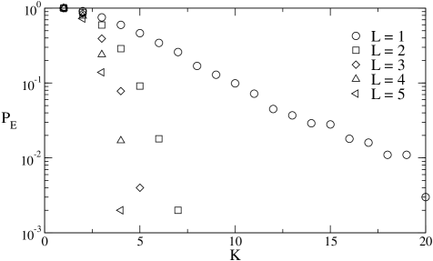
Abbildung 4.2: Success probability $P_{E}$ of the geometric attack as a function of $K$. Symbols denote results obtained in $1000$ simulations using the random walk learning rule and $N=1000$.

Consequently, A and B can achieve security against this attack not only by increasing the synaptic depth $L$, but also by using a greater number of hidden units $K$. Of course, for $K>3$ large values of $L$ are not possible, as the process of synchronization is then driven by fluctuations. Nevertheless, figure 4.2 shows that the success probability $P_{E}$ for the geometric attack drops quickly with increasing $K$ even in the case $L=1$.

As the geometric attack is an element of both advanced attacks, majority attack and genetic attack, one can also defeat these methods by increasing $K$. But then synchronization by mutual interaction and learning by listening become more and more similar. Thus one has to look at the success probability of the simple attack, too.

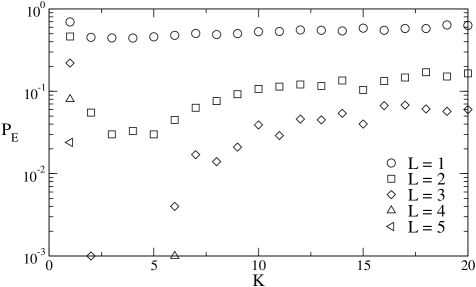
Abbildung 4.3: Success probability $P_{E}$ of the simple attack as a function of $K$. Symbols denote results obtained in $1000$ simulations using the random walk learning rule and $N=1000$.

As this method does not correct the outputs $\sigma_{i}^{E}$ of the hidden units at all, the distance between the fixed point at $\rho_{\mathrm{f}}<1$ of the dynamics and the absorbing state at $\rho=1$ is greater than in the case of the geometric attack. That is why a simple attacker needs larger fluctuations to synchronize and is less successful than the more advanced attack as long as the number of hidden units is small.

In principle, scaling law (4.7) is also valid for this method. But one cannot find a single successful simple attack in $1000$ simulations using the parameters $K=3$ and $L=3$ [13]. This is clearly visible in figure 4.3. Consequently, the simple attack is not sufficient to break the security of the neural key-exchange protocol for $K\leq 3$.

But learning by listening without any correction works if the number of hidden units is large. Here the probability of repulsive steps is similar for both bidirectional and unidirectional interaction as shown in section 3.2. That is why $P_{E}$ approaches a non-zero constant value in the limit $K\rightarrow\infty$.

These results show that $K=3$ is the optimal choice for the cryptographic application of neural synchronization. $K=1$ and $K=2$ are too insecure in regard to the geometric attack. And for $K>3$ the effort of A and B grows exponentially with increasing $L$, while the simple attack is quite successful in the limit $K\rightarrow\infty$. Consequently, one should only use Tree Parity Machines with three hidden units for the neural key-exchange protocol.

4.1.2 Genetic attack

In the case of the genetic attack E’s success depends mainly on the ability to determine the fitness of her neural networks. Of course, the best quantity for this purpose would be the overlap $\rho^{AE}$ between an attacking network and A’s Tree Parity Machine. However, it is not available, as E only knows the weight vectors of her own networks. Instead the attacker uses the frequency of the event $\tau^{E}=\tau^{A}$ in recent steps, which gives a rough estimate of $\rho^{AE}$.

Therefore a selection step only works correctly, if there are clear differences between attractive and repulsive effects. As the step sizes $\langle\Delta\rho_{\mathrm{a}}\rangle$ and $\langle\Delta\rho_{\mathrm{r}}\rangle$ decrease proportional to $L^{-2}$, distinguishing both step types becomes more and more complicated for E. Thus one expects a similar asymptotic behavior of $P_{E}$ in the limit $L\rightarrow\infty$ as observed before.

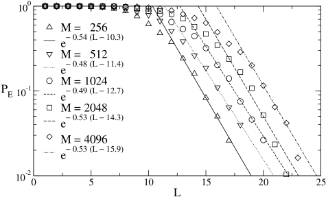
Abbildung 4.4: Success probability of the genetic attack. Symbols denote results obtained in $1000$ simulations with $K=3$, $N=1000$, and random walk learning rule. The lines show fit results using (4.8) as a model.

Figure 4.4 shows that this is indeed the case. The success probability drops exponentially with increasing synaptic depth $L$,

$$P_{E}\sim e^{-y(L-L_{0})}\,,$$ (4.8)

as long as $L>L_{0}$ [22]. But for $L<L_{0}$ E is nearly always successful. Consequently, A and B have to use Tree Parity Machines with large synaptic depth in order to secure the key-exchange protocol against this attack.

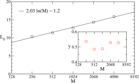
Abbildung 4.5: Coefficients $L_{0}$ and $y$ for the genetic attack as a function of the number of attackers $M$. Symbols denote the results obtained in figure 4.4 for $K=3$, $N=1000$, and random walk learning rule.

In contrast to the geometric method, E is able to improve her success probability by increasing the maximum number of networks used for the genetic attack. As shown in figure 4.5 this changes $L_{0}$, but the coefficient $y$ remains approximately constant. However, it is a logarithmic effect:

$$L_{0}(M)=L_{0}(1)+L_{E}\ln M\,.$$ (4.9)

That is why the attacker has to increase the number of her Tree Parity Machines exponentially,

$$M\propto e^{L/L_{E}}$$ (4.10)

in order to compensate a change of $L$ and maintain a constant success probability $P_{E}$. But the effort needed to generate a key only increases proportional to $L^{2}$. Consequently, the neural key-exchange protocol is secure against the genetic attack in the limit $L\rightarrow\infty$.

4.1.3 Majority attack

An opponent who has an ensemble of $M$ Tree Parity Machines, can also use the majority attack to improve $P_{E}$. This method does neither generate variants nor select the fittest networks, so that their number remains constant throughout the process of synchronization. Instead the majority decision of the $M$ Tree Parity Machines determines the internal representation $(\sigma_{1}^{E},\dots,\sigma_{K}^{E})$ used for the purpose of learning. Therefore this algorithm implements, in fact, the optimal Bayes learning rule [28, 35, 36].

In order to describe the state of the ensemble one can use two order parameters. First, the mean value of the overlap between corresponding hidden units in A’s and E’s neural networks,

$$\rho_{i}^{AE}=\frac{1}{M}\sum_{m=1}^{M}\frac{\mathbf{w}_{i}^{A}\cdot\mathbf{w}_{i}^{E,m}}{||\mathbf{w}_{i}^{A}||\,||\mathbf{w}_{i}^{E,m}||}\,,$$ (4.11)

indicates the level of synchronization. Here the index $m$ denotes the $m$-th attacking network. Similar to other attacks, E starts without knowledge in regard to A, so that $\rho^{AE}=0$ at the beginning. And finally she is successful, if $\rho^{AE}=1$ is reached.

Second, the average overlap between two attacking networks,

$$\rho_{i}^{EE}=\frac{1}{M(M-1)}\sum_{m=1}^{M}\sum_{n\not=m}\frac{\mathbf{w}_{i}^{E,m}\cdot\mathbf{w}_{i}^{E,n}}{||\mathbf{w}_{i}^{E,m}||\,||\mathbf{w}_{i}^{E,n}||}\,,$$ (4.12)

describes the correlations in E’s ensemble. At the beginning of the synchronization $\rho^{EE}=0$, because all weights are initialized randomly and uncorrelated. But as soon as $\rho^{EE}=1$ is reached, E’s networks are identical, so that the performance of the majority attack is reduced to that of the geometric method.

In the large $M$ limit, the majority vote of the ensemble is identical to the output values $\sigma_{i}$ of a single neural network, which is located at the center of mass [35]. Its weight vectors are given by the normalized average over all of E’s Tree Parity Machines:

$$\mathbf{w}_{i}^{E,\mathrm{cm}}=\frac{1}{M}\sum_{m=1}^{M}\frac{\mathbf{w}_{i}^{E,m}}{||\mathbf{w}_{i}^{E,m}||}\,.$$ (4.13)

The normalization of $\mathbf{w}_{i}^{E,m}$ corresponds to the fact that each member has exactly one vote. Using (4.11) and (4.12) one can calculate the overlap between the center of mass and A’s tree Parity Machine:

$$\rho_{i}^{\mathrm{cm}}=\frac{\mathbf{w}_{i}^{A}\cdot\mathbf{w}_{i}^{E,\mathrm{cm}}}{||\mathbf{w}_{i}^{A}||\,||\mathbf{w}_{i}^{E,\mathrm{cm}}||}=\frac{\rho_{i}^{AE}}{\sqrt{\rho_{i}^{EE}+\frac{1}{M}\left(1-\rho_{i}^{EE}\right)}}\,.$$ (4.14)

Consequently, the effective overlap between A and E is given by

$$\rho_{i}^{\mathrm{cm}}\sim\frac{\rho_{i}^{AE}}{\sqrt{\rho_{i}^{EE}}}$$ (4.15)

in the limit $M\rightarrow\infty$. This result is important for the dynamics of the synchronization process between A and E, because $\rho_{i}^{\mathrm{cm}}$ replaces $\rho_{i}^{AE}$ in the calculation of the transition probabilities $P_{\mathrm{a}}(\rho)$ and $P_{\mathrm{r}}(\rho)$, whenever the majority vote is used to adjust the weights. But the step sizes $\langle\Delta\rho_{\mathrm{a}}(\rho)\rangle$ and $\langle\Delta\rho_{\mathrm{r}}(\rho)\rangle$ are not affected by this modification of the algorithm. Therefore the average change of the overlap between A and E is given by

$$\langle\Delta\rho_{i}^{AE}\rangle=P_{\mathrm{a}}(\rho_{i}^{\mathrm{cm}})\langle\Delta\rho_{\mathrm{a}}(\rho_{i}^{AE})\rangle+P_{\mathrm{r}}(\rho_{i}^{\mathrm{cm}})\langle\Delta\rho_{\mathrm{r}}(\rho_{i}^{AE})\rangle\,,$$ (4.16)

if the majority vote is used for updating the weight vectors. Although this equation is strictly correct only in the limit $M\rightarrow\infty$, $M=100$ is already sufficient for the majority attack [21].

However, as all attacking networks learn the same internal representation, the internal overlap $\rho_{i}^{EE}$ is increased by the resulting attractive effect:

$$\langle\Delta\rho_{i}^{EE}\rangle=\frac{1}{2}\,\langle\Delta\rho_{\mathrm{a}}(\rho_{i}^{EE})\rangle\,.$$ (4.17)

Hence $\rho_{i}^{EE}$ grows faster than $\rho_{i}^{AE}$ in these steps, so that the advantage of the majority vote decreases whenever it is used [37].

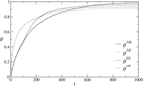
Abbildung 4.6: Process of synchronization in the case of a majority attack with $M=100$ attacking networks, averaged over $1000$ simulations for $K=3$, $L=5$, $N=1000$, and random walk learning rule.

This is clearly visible in figure 4.6. In the first $100$ steps the attacker only uses the geometric attack. Here $\rho^{EE}\approx\rho^{AE}$, which can also be observed for an ensemble of perceptrons learning according to the Bayes rule [28]. At $t=100$, using the majority vote gives E a huge advantage compared to the geometric attack, because $\rho^{\mathrm{cm}}\approx\sqrt{\rho^{AE}}>\rho^{AE}$, so that the probability of repulsive steps is reduced. Therefore the attacker is able to maintain $\rho^{AE}\approx\rho^{AB}$ for some time. Later $\rho^{EE}$ increases and this benefit vanishes.

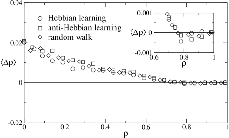
Abbildung 4.7: Average change of the overlap for the majority attack with $M=100$ attacking networks. Symbols denote results obtained in $200$ simulations using $K=3$, $L=5$, and $N=1000$.

However, the attacker is unable to reach full synchronization on average. As shown in figure 4.7, there is still a fixed point at $\rho_{\mathrm{f}}<1$ in the case of the majority attack, although its distance to the absorbing state is smaller than for the geometric attack. Consequently, one expects a higher success probability $P_{E}$, but similar scaling behavior.

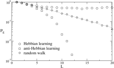
Abbildung 4.8: Success probability $P_{E}$ of the majority attack with $M=100$ attacking networks for $K=3$ and $N=1000$. Symbols denote results obtained in $10\,000$ simulations and the line shows the corresponding fit from figure 4.9.

Figure 4.8 shows that this is indeed the case for the random walk learning rule and for anti-Hebbian learning. But if A and B use the Hebbian learning rule instead, $P_{E}$ reaches a constant non-zero value in the limit $L\rightarrow\infty$ [21]. Apparently, the change of the weight distribution caused by Hebbian learning is enough to break the security of the neural key-exchange protocol. Consequently, A and B cannot use this learning rule for cryptographic purposes.

While anti-Hebbian learning is secure against the majority attack, a lot of finite size effects occur in smaller systems, which do not fulfill the condition $L\ll\sqrt{N}$. In this case $\langle t_{\mathrm{sync}}\rangle$ increases faster than $L^{2}$ as shown in section 3.5. Fortunately, A and B can avoid this problem by just using the random walk learning rule.

4.1.4 Comparison of the attacks

As E knows the parameters of the neural key-exchange protocol, she is able to select the best method for an attack. Consequently, one has to compare the available attacks in order to determine the maximum of $P_{E}$.

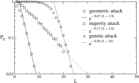
Abbildung 4.9: Success probability of different attacks as a function of the synaptic depth $L$. Symbols denote results obtained in $1000$ simulations using the random walk learning rule, $K=3$, and $N=1000$, while the lines show fit results using model (4.8). The number of attacking networks is $M=4096$ for the genetic attack and $M=100$ for the majority attack.

Figure 4.9 shows the result. Here (4.8) has been used as fit model even for the geometric attack, which is a special case of both advanced attacks for $M=1$. Of course, by doing so the curvature visible in figure 4.1 is neglected, so that extrapolating $P_{E}$ for $L\rightarrow\infty$ overestimates the efficiency of this method.

All three attacks have similar scaling behavior, but the coefficients $L_{0}$ and $y$ obtained by fitting with (4.8) depend on the chosen method. The geometric attack is the simplest method considered in figure 4.9. Therefore its success probability is lower than for the more advanced methods. As the exponent $y$ is large, A and B can easily secure the key-exchange protocol against this method by just increasing $L$.

In the case of the majority attack, $P_{E}$ is higher, because the cooperation between the attacking networks reduces the coefficient $y$. A and B have to compensate this by further stepping up $L$. In contrast, the genetic attack merely increases $L_{0}$, but $y$ does not change significantly compared to the geometric attack. Therefore the genetic attack is only better if $L$ is not too large. Otherwise E gains most by using the majority attack [22].

While A and B can reach any desired level of security by increasing the synaptic depth, this is difficult to realize in practise. Extrapolation of (4.8) shows clearly that $P_{E}\approx 10^{-4}$ is achieved for $K=3$, $L=57$, $N=1000$, and random walk learning rule. But the average synchronization time $\langle t_{\mathrm{sync}}\rangle\approx 1.6\cdot 10^{5}$ is quite large in this case. Consequently, it is reasonable to develop an improved neural key-exchange protocol [24, 19, 23], which is the topic of chapter 5.

4.2 Security by interaction

The main difference between the partners and the attacker in neural cryptography is that A and B are able to influence each other by communicating their output bits $\tau^{A}$ and $\tau^{B}$, while E can only listen to these messages. Of course, A and B use their advantage to select suitable input vectors for adjusting the weights. As shown in chapter 3 this finally leads to different synchronization times for partners and attackers.

However, there are more effects, which show that the two-way communication between A and B makes attacking the neural key-exchange protocol more difficult than simple learning of examples. These confirm that the security of neural cryptography is based on the bidirectional interaction of the partners.

4.2.1 Version space

The time series of pairs $(\tau^{A},\tau^{B})$ of output bits produced by two interacting Tree Parity Machines depends not only on the sequence of input vectors $\mathbf{x}_{i}(t)$, but also on the initial weight vectors $\mathbf{w}_{i}^{A/B}(0)$ of both neural networks. Of course, E can reproduce the time series $\tau^{B}(t)$ exactly, if she uses a third Tree Parity Machine with $\mathbf{w}_{i}^{E}(0)=\mathbf{w}_{i}^{B}(0)$, because the learning rules are deterministic. But choosing other initial values for the weights in E’s neural network may lead to the same sequence of output bits. The set of initial configurations with this property is called version space [28]. Its size $n_{\mathrm{vs}}$ is a monotonically decreasing function of the length $t$ of the sequence, because each new element $\mathbf{x}_{i}(t)$ imposes an additional condition on $\mathbf{w}_{i}^{E}(0)$. Of course, it does not matter whether E uses the simple attack or the geometric attack, as both algorithms are identical under the condition $\tau^{E}(t)=\tau^{B}(t)$.

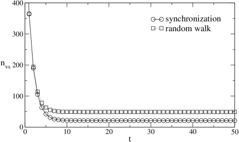
Abbildung 4.10: Version space of interacting Tree Parity Machines with $K=3$, $L=1$, $N=2$, and random walk learning rule, averaged over $1000$ simulations.

Figure 4.10 shows that the size of the version space shrinks by a factor $1/2$ in each step at the beginning of the time series. Here the possible configurations of the weights are still uniformly distributed, so that each output $\tau^{B}$ gives one bit of information about the initial conditions.

But later neural networks which have started with similar weight vectors synchronize. That is why the configurations are no longer uniformly distributed and the shrinking of the $n_{\mathrm{vs}}$ becomes slower and slower. Finally, all Tree Parity Machines in the version space have synchronized with each other. From then on $n_{\mathrm{vs}}$ stays constant.

However, the size of the version space in the limit $t\rightarrow\infty$ depends on the properties of the time series. If A and B start fully synchronized, they do not need to influence each other and all input vectors in the sequence are used to update the weights. In this case E has to learn randomly chosen examples of a time-dependent rule [6]. In contrast, if A and B start with uncorrelated weight vectors, they select a part of the input sequence for adjusting their weights. For them this interaction increases the speed of the synchronization process, because only suitable input vectors remain. But it also decreases $n_{\mathrm{vs}}(t\rightarrow\infty)$, so that imitating B is more difficult for E.

Consequently, the two-way communication between the partners gives them an advantage, which cannot be exploited by a passive attacker. Therefore bidirectional interaction is important for the security of the neural key-exchange protocol.

4.2.2 Mutual information

Instead of using the overlap $\rho$ as order parameter, which is closely related to the dynamics of the neural networks and the theory of learning, one can look at the process of synchronization from the point of view of information theory, too. For this purpose, the mutual information $I^{AB}(t)$ defined in (2.18) describes A’s and B’s knowledge about each other. Similarly $I^{AE}(t)$ measures, how much information E has gained in regard to A at time $t$ by listening to the communication of the partners.

All participants start with zero knowledge about each other, so that $I^{AB}=0$ and $I^{AE}=0$ at the beginning of the key exchange. In each step there are several sources of information. The input vectors $\mathbf{x}_{i}(t)$ determine, in which directions the weights are moved, if the learning rule is applied. And, together with the outputs $\tau^{A}(t)$ and $\tau^{B}(t)$, they form an example, which gives some information about the current weight vectors in A’s and B’s Tree Parity Machines. Although all participants have access to $\mathbf{x}_{i}(t)$, $\tau^{A}(t)$, and $\tau^{B}(t)$, the increase of the mutual information $I$ depends on the algorithm used to adjust the weights.

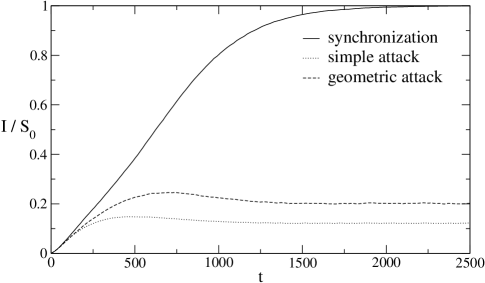
Abbildung 4.11: Mutual information between partners and attackers. Symbols denote simulation results for $K=3$, $L=5$, $N=1000$, and random walk learning rule, while the lines show the results of corresponding iterative calculations for $N\rightarrow\infty$.

This is clearly visible in figure 4.11. While the partners reach full synchronization with $I^{AB}=S_{0}$ quickly, the attacker is much slower. And E performs better if she uses the geometric method instead of the simple attack. Of course, these observations correspond to those presented in chapter 3.

While the differences between E’s attack methods are caused by the learning algorithms, which transform the available information into more or less knowledge about A’s and B’s weights, this is not the only reason for $I^{AE}(t)<I^{AB}(t)$. In order to synchronize the partners have to agree on some weight vectors $\mathbf{w}_{i}$, which are, in fact, functions of the sequence $\mathbf{x}_{i}(t)$ and the initial conditions $\mathbf{w}_{i}^{A/B}(0)$. So they already have some information, which they share during the process of synchronization. Therefore the partners gain more mutual information $I$ from each message than an attacker, who has no prior knowledge about the outcome of the key exchange. Consequently, it is the bidirectional interaction which gives A and B an advantage over E.

4.3 Number of keys

Although all attacks on the neural key-exchange protocol known up to now are based on the training of Tree Parity Machines with examples generated by the partners A and B, this is not a necessary condition. Instead of that the opponent could try a brute-force attack. Of course, a success of this method is nearly impossible without additional information, as there are $(2L+1)^{KN}$ different configurations for the weights of a Tree Parity Machine. However, E could use some clever algorithm to determine which keys are generated with high probability for a given input sequence. Trying out these would be a feasible task as long as there are not too many. Consequently, a large number of keys is important for the security of neural cryptography, especially against brute-force attacks.

4.3.1 Synchronization without interaction

If the weights are chosen randomly, there are $(2L+1)^{2KN}$ possible configurations for a pair of Tree Parity Machines. But the neural key-exchange protocol can generate at most $(2L+1)^{KN}$ different keys. Consequently, sets of different initial conditions exist, which lead to identical results. That is why synchronization even occurs without any interaction between neural networks besides a common sequence of input vectors.

In order to analyze this effect the following system consisting of two pairs of Tree Parity Machines is used:

$$\mathbf{w}_{i}^{A+} = g(\mathbf{w}_{i}^{A}+f(\sigma_{i}^{A},\tau^{A},\tau^{B})\mathbf{x}_{i})\,,$$ (4.18)

$$\mathbf{w}_{i}^{B+} = g(\mathbf{w}_{i}^{B}+f(\sigma_{i}^{B},\tau^{A},\tau^{B})\mathbf{x}_{i})\,,$$ (4.19)

$$\mathbf{w}_{i}^{C+} = g(\mathbf{w}_{i}^{C}+f(\sigma_{i}^{C},\tau^{C},\tau^{D})\mathbf{x}_{i})\,,$$ (4.20)

$$\mathbf{w}_{i}^{D+} = g(\mathbf{w}_{i}^{D}+f(\sigma_{i}^{D},\tau^{C},\tau^{D})\mathbf{x}_{i})\,.$$ (4.21)

All four neural networks receive the same sequence of input vectors $\mathbf{x}_{i}$, but both pairs communicate their output bits only internally. Thus A and B as well as C and D synchronize using one of the available learning rules, while correlations caused by common inputs are visible in the overlap $\rho_{i}^{AC}$. Because of the symmetry in this system, $\rho_{i}^{AD}$, $\rho_{i}^{BC}$, and $\rho_{i}^{BD}$ have the same properties as this quantity, so that it is sufficient to look at $\rho_{i}^{AC}$ only.

Of course, synchronization of networks which do not interact with each other, is much more difficult and takes a longer time than performing the normal key-exchange protocol. Thus full internal synchronization of the pairs usually happens well before A’s and C’s weight vectors become identical, so that $\rho_{i}^{AB}=1$ and $\rho_{i}^{CD}=1$ are assumed for the calculation of $\langle\Delta\rho_{i}^{AC}(\rho_{i}^{AC})\rangle$.

As before, both attractive and repulsive steps are possible. In the case of identical overlap between corresponding hidden units, random walk learning rule, and $K>1$, the probability of these step types is given by:

$$P_{\mathrm{a}} = \frac{1}{2}\sum_{i=0}^{(K-1)/2}{K-1\choose 2i}(1-\epsilon)^{K-2i}\,\epsilon^{2i}$$ (4.22)

$$+ \frac{1}{2}\sum_{i=0}^{(K-1)/2}{K-1\choose 2i}(1-\epsilon)^{K-2i-1}\epsilon^{2i+1}\,,$$

$$P_{\mathrm{r}} = \sum_{i=1}^{K/2}{K-1\choose 2i-1}(1-\epsilon)^{K-2i}\epsilon^{2i}$$ (4.23)

$$+ \sum_{i=1}^{K/2}{K-1\choose 2i-1}(1-\epsilon)^{K-2i+1}\,\epsilon^{2i-1}\,.$$

Here $\epsilon$ denotes the generalization error defined in equation (3.20) in regard to $\rho^{AC}$. For $K=1$ only attractive steps occur, so that $P_{\mathrm{a}}=1$, which is similar to the geometric attack. But in the case of $K=3$, one finds

$$P_{\mathrm{a}} = \frac{1}{2}\left[1-2(1-\epsilon)\epsilon\right]\,,$$ (4.24)

$$P_{\mathrm{r}} = 2(1-\epsilon)\epsilon\,.$$ (4.25)

As long as $\rho^{AC}>0$ the probability of repulsive steps is higher than $P_{\mathrm{r}}^{E}=\epsilon$ for the simple attack. Consequently, one expects that the dynamics of $\rho^{AC}$ has a fixed point at $\rho_{\mathrm{f}}^{AC}<\rho_{\mathrm{f}}^{E}<1$ and synchronization is only possible by fluctuations.

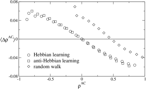
Abbildung 4.12: Average change of the overlap between A and C for $K=3$, $L=3$, and $N=1000$, obtained in $100$ simulations with $100$ pairs of neural networks.

Figure 4.12 shows that this is indeed the case. As more repulsive steps occur, the probability for full synchronization here is much smaller than for a successful simple attack. In fact, large enough fluctuations which lead from $\rho^{AC}=0$ to $\rho^{AC}=1$ without interaction only occur in small systems. But the common input sequence causes correlations between $\mathbf{w}_{i}^{A}$ and $\mathbf{w}_{i}^{C}$ even for $L\gg 1$ and $N\gg 1$.

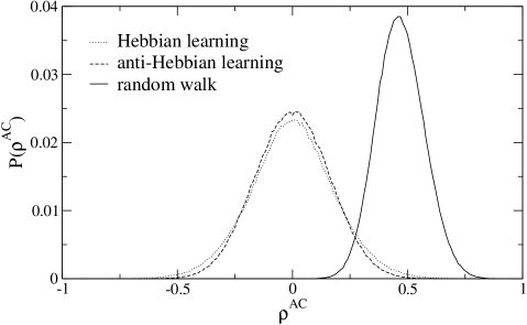
Abbildung 4.13: Distribution of the overlap $\rho^{AC}$ after $1000$ steps for $K=3$, $L=3$, and $N=100$, obtained in $100$ simulations with $100$ pairs of Tree Parity Machines.

This is clearly visible in figure 4.13. However, if Hebbian or anti-Hebbian learning is used instead of the random walk learning rule, one observes a somewhat different behavior: the fixed point of the dynamics for $K=3$ is located at $\rho_{\mathrm{f}}=0$. According to these two learning rules the weights of corresponding hidden units move in opposite directions, if both $\tau^{A}\not=\tau^{C}$ and $\sigma_{i}^{A}\not=\sigma_{i}^{C}$. The average step size of such an inverse attractive step is given by

$$\langle\Delta\rho_{\mathrm{i}}(\rho)\rangle=-\langle\Delta\rho_{\mathrm{a}}(-\rho)\rangle\,.$$ (4.26)

While $P_{\mathrm{r}}$ is independent of the learning rule, one finds

$$P_{\mathrm{a}} = \frac{1}{2}\sum_{i=0}^{(K-1)/2}{K-1\choose 2i}(1-\epsilon)^{K-2i}\,\epsilon^{2i}\,,$$ (4.27)

$$P_{\mathrm{i}} = \frac{1}{2}\sum_{i=0}^{(K-1)/2}{K-1\choose 2i}(1-\epsilon)^{K-2i-1}\epsilon^{2i+1}$$ (4.28)

for Hebbian or anti-Hebbian learning and $K>1$. If $K$ is odd, the effects of all types of steps cancel out exactly at $\rho=0$, because $\langle\Delta\rho_{\mathrm{r}}(0)\rangle=0$ and $P_{\mathrm{i}}(0)=P_{\mathrm{a}}(0)$. Otherwise, the two transition probabilities, $P_{\mathrm{a}}(0)$ for attractive steps and $P_{\mathrm{i}}(0)$ for inverse attractive steps, are only approximately equal. Thus one observes $\rho_{\mathrm{f}}\approx 0$ independent of $K$, so that the correlations between A and C are smaller in this case than for the random walk learning rule.

But if the initial overlap between A and C is already large, it is very likely that both pairs of Tree Parity Machines generate the same key regardless of the learning rule. Consequently, the number of keys $n_{\mathrm{key}}$ is smaller than the number of weight configurations $n_{\mathrm{conf}}=(2L+1)^{KN}$ of a Tree Parity Machine.

4.3.2 Effective key length

In order to further analyze the correlations between A’s and C’s neural networks the entropy

$$S^{AC}=\sum_{i=1}^{K}S_{i}^{AC}$$ (4.29)

of their weight distribution is used. Here $S_{i}^{AC}$ is the entropy of a single hidden unit defined in (2.15). Of course, one can assume here that the weights stay uniformly distributed during the process of synchronization, either because the system size is large ($N\gg 1$) or the random walk learning rule is used. Therefore the entropy of a single network is given by $S_{0}=KN\ln(2L+1)$.

Consequently, $S^{AC}-S_{0}$ is the part of the total entropy, which describes the correlations caused by using a common input sequence. It is proportional to the effective length of the generated cryptographic key,

$$l_{\mathrm{key}}=\frac{S^{AC}-S_{0}}{\ln 2}\,,$$ (4.30)

which would be the average number of bits needed to represent it using both an optimal encoding without redundancy and the input sequence as additional knowledge. If the possible results of the neural key-exchange protocol are uniformly distributed, each one can be represented by a number consisting of $l_{\mathrm{key}}$ bits. In this case

$$n_{\mathrm{key}}=2^{l_{\mathrm{key}}}=e^{S^{AC}-S_{0}}$$ (4.31)

describes exactly the number of keys which can be generated using different initial weights for the same input sequence. Otherwise, the real number is larger, because mainly configurations, which occur with high probability, are relevant for the calculation of $S^{AC}$. However, an attacker is only interested in those prevalent keys. Therefore $n_{\mathrm{key}}$ as defined in equation (4.31) is, in fact, a lower bound for the number of cryptographic relevant configurations.

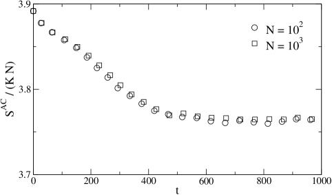
Abbildung 4.14: Entropy per weight for A and C for $K=3$, $L=3$, and random walk learning rule, obtained in $100$ simulations with $100$ pairs of neural networks.

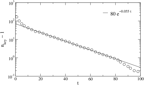
Abbildung 4.15: Number of keys for $K=3$, $L=1$, $N=2$, and random walk learning rule, obtained by exhaustive search and averaged over $100$ random input sequences.

Figure 4.14 shows the time evolution of the entropy. First $S^{AC}$ shrinks linearly with increasing $t$, as the overlap $\rho$ between A and C grows, while it approaches the stationary state. This behavior is consistent with an exponentially decreasing number of keys, which can be directly observed in very small systems as shown in figure 4.15. Of course, after the system has reached the fixed point, the entropy stays constant. This minimum value of the entropy is then used to determine the effective number $n_{\mathrm{key}}$ of keys according to (4.31).

It is clearly visible that there are two scaling relations for $S^{AC}$:

• Entropy is an extensive quantity. Thus both $S^{AC}$ and $S_{0}$ are proportional to the number of weights $N$. Consequently, the number of keys, which can be generated by the neural key-exchange protocol for a given input sequence, grows exponentially with increasing system size $N$.

• The relevant time scale for all processes related to the synchronization of Tree Parity Machines is defined by the step sizes of attractive and repulsive steps which are asymptotically proportional to $L^{-2}$. Therefore the time needed to reach the fixed point $\rho_{\mathrm{f}}^{AC}$ is proportional to $L^{2}$, similar to $\langle t_{\mathrm{sync}}\rangle$. In fact, it is even of the same order as the average synchronization time.

Instead of using the entropy directly, it is better to look at the mutual information $I^{AC}=2S_{0}-S^{AC}$ shared by A and C, which comes from the common input sequence and is visible in the correlations of the weight vectors. Using (2.19) and (4.31) leads to [31]

$$I^{AC}=-\ln\left(\frac{n_{\mathrm{key}}}{n_{\mathrm{conf}}}\right)\,.$$ (4.32)

Therefore the effective number of keys is given by

$$n_{\mathrm{key}}=n_{\mathrm{conf}}\,e^{-I^{AC}}=(2L+1)^{KN}e^{-I^{AC}}\,.$$ (4.33)

As shown in figure 4.16 the mutual information $I^{AC}$ at the end of the synchronization process becomes asymptotically independent of the synaptic depth in the limit $L\rightarrow\infty$. Consequently, the ratio $n_{\mathrm{key}}/n_{\mathrm{conf}}$ is constant except for finite-size effects occurring in small systems.

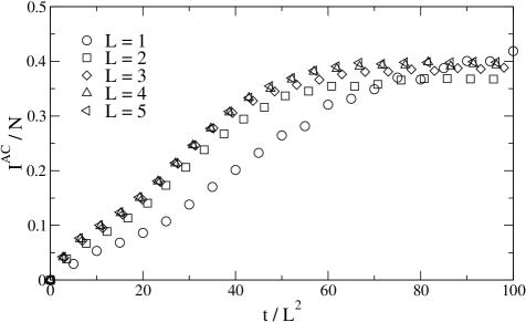
Abbildung 4.16: Mutual information between A and C for $K=3$, $N=1000$, and random walk learning rule, obtained in $1000$ simulations with $10$ pairs of neural networks.

Abbildung 4.17: Extrapolation of $I^{AC}$ for $K=3$, $L\rightarrow\infty$, and $N=1000$. Symbols denote the average value of $I^{AC}(t)$ in the range $80\,L^{2}\leq t\leq 100\,L^{2}$, which has been obtained in $1000$ simulations with $10$ pairs of neural networks.

The amount of correlations between A and C depends on the distribution of the overlap $\rho^{AC}$ in the steady state, which can be described by its average value $\rho_{\mathrm{f}}$ and its standard deviation $\sigma_{\mathrm{f}}$. As before, $\sigma_{\mathrm{f}}$ decreases proportional to $L^{-1}$ due to diminishing fluctuations in the limit $L\rightarrow\infty$, while $\rho_{\mathrm{f}}$ stays nearly constant. Hence $I^{AC}$ consists of two parts, one independent of $L$ and one proportional to $L^{-1}$ as shown in figure 4.17.

In the case of the random walk learning rule the mutual information increases with $L$, because fluctuations are reduced which just disturb the correlations created by the common sequence of input vectors. Extrapolating $I^{AC}$ yields the result [31]

$$n_{\mathrm{key}}\approx\left[0.66(2L+1)^{3}\right]^{N}\,,$$ (4.34)

which is valid for $K=3$ and $1\ll L\ll\sqrt{N}$. Consequently, $n_{\mathrm{key}}$ grows exponentially with $N$, so that there are always enough possible keys in larger systems to prevent successful brute-force attacks on the neural key-exchange protocol.

Using Hebbian or anti-Hebbian learning, however, improves the situation further. Because of $\rho_{\mathrm{f}}=0$ one finds $n_{\mathrm{key}}\rightarrow n_{\mathrm{conf}}$ in the limit $L\rightarrow\infty$. Therefore the input sequence does not restrict the set of possible keys in very large systems using $K=3$, $1\ll L\ll\sqrt{N}$, and one of these two learning rules.

4.4 Secret inputs

The results of section 4.3 indicate that the input vectors are an important source of information for the attacker. Thus keeping $\mathbf{x}_{i}$ at least partially secret should improve the security of the neural key-exchange protocol.

4.4.1 Feedback mechanism

In order to reduce the amount of input vectors transmitted over the public channel, the partners have to use an alternative source for the input bits. For that purpose they can modify the structure of the Tree Parity Machines, which is shown in figure 4.18 [19].

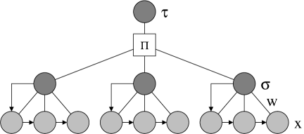
Abbildung 4.18: A Tree Parity Machine with $K=3$, $N=3$, and feedback.

Here the generation of the input values is different. Of course, A and B still start with a set of $K$ randomly chosen public inputs $\mathbf{x}_{i}$. But in the following time steps each input vector is shifted,

$$x_{i,j}^{A/B+}=x_{i,j-1}^{A/B}\quad\mbox{for $j>1$,}$$ (4.35)

and the output bit $\sigma_{i}$ of the corresponding hidden unit is used as the new first component,

$$x_{i,1}^{A/B+}=\sigma_{i}^{A/B}\,.$$ (4.36)

This feedback mechanism [38] replaces the public sequence of random input vectors. Additionally, the anti-Hebbian learning rule (2.7) is used to update the weights. By doing so one avoids the generation of trivial keys, which would be the result of the other learning rules [19]. Thus the hidden units of both Tree Parity Machines work as confused bit generators [39].

Abbildung 4.19: Probability of synchronization for two Tree Parity Machines with feedback as a function of the initial overlap $\rho_{\mathrm{start}}$. Symbols denote results obtained in $1000$ simulations with $K=3$, $L=3$, and $N=100$.

However, synchronization is not possible without further information, as the bit sequence produced by such a neural network is unpredictable [38, 40, 41] for another one of the same type [39, 19]. This is clearly visible in figure 4.19. The reason is that the input vectors of A’s and B’s Tree Parity Machines become more and more different, because each occurrence of $\sigma_{i}^{A}\not=\sigma_{i}^{B}$ reduces the number of identical input bits by one for the next $N$ steps. Of course, the partners disagree on the outputs $\sigma_{i}$ quite often at the beginning of the synchronization process, so that they soon have completely uncorrelated input vectors and mutual learning is no longer possible.

4.4.2 Synchronization with feedback

As the feedback mechanism destroys the common information about the inputs of the Tree Parity Machines, an additional mechanism is necessary for synchronization, which compensates this detrimental effect sufficiently. For that purpose A and B occasionally reset the input vectors of their Tree Parity Machines if too many steps with $\tau^{A}\not=\tau^{B}$ occur.

In fact, the following algorithm is used [19]:

• If $\tau^{A}=\tau^{B}$, the weights are updated according to the anti-Hebbian learning rule (2.7) and the feedback mechanism is used to generate the next input.

• If the output bits disagree, $\tau^{A}\not=\tau^{B}$, the input vectors are shifted, too, but all pairs of input bits $x_{i,1}^{A/B}$ are set to common public random values.

• After $R$ steps with different output, $\tau^{A}\not=\tau^{B}$, all inputs are reinitialized using a set of $K$ randomly chosen public input vectors.

Of course, setting $R=0$ leads to synchronization without feedback, while no synchronization is possible in the limit $R\rightarrow\infty$.

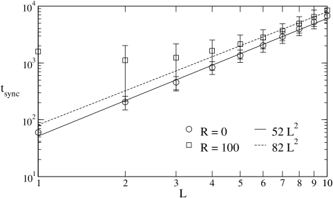
Abbildung 4.20: Average synchronization time and its standard deviation for neural cryptography with feedback, obtained in $10\,000$ simulations with $K=3$ and $N=10\,000$.

Figure 4.20 shows that using the feedback mechanism increases the average number of steps needed to achieve full synchronization. While there are strong finite size-effects, the scaling relation $\langle t_{\mathrm{sync}}\rangle\propto L^{2}$ is still valid for $1\ll L\ll\sqrt{N}$. Only the constant of proportionality is larger than before [19].

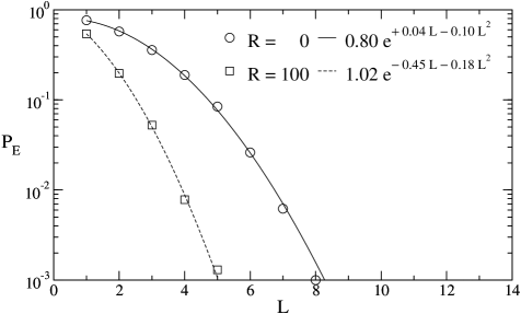
Abbildung 4.21: Success probability $P_{E}$ of the geometric attack as a function of the synaptic depth $L$. Symbols denote results averaged over $10\,000$ simulations for $K=3$ and $N=1000$.

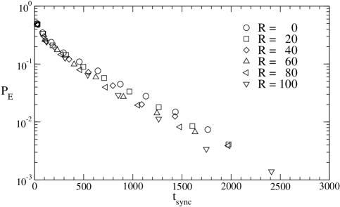
Abbildung 4.22: Success probability $P_{E}$ of the geometric attack as a function of the average synchronization time $\langle t_{\mathrm{sync}}\rangle$. Symbols denote results of $10\,000$ iterative calculations for $K=3$ and $N\rightarrow\infty$. Here successful synchronization has been defined as $\rho>0.9$ [19].

As shown in figure 4.21 a similar result can be observed in regard to the success probability of the geometric attack. As before, $P_{E}$ drops exponentially with increasing synaptic depth, so that A and B can achieve any desired level of security by changing $L$. But with feedback smaller values of $L$ are sufficient, because the factors $y_{1}$ and $y_{2}$ in the scaling law (4.7) are larger. Therefore using the feedback mechanism improves the security of neural cryptography by keeping input values partially secret.

However, A and B usually want to keep their effort constant. Then one has to look at the function $P_{E}(\langle t_{\mathrm{sync}}\rangle)$ instead of $P_{E}(L)$, which is plotted in figure 4.22 for several values of the feedback parameter $R$. It is clearly visible that $P_{E}(\langle t_{\mathrm{sync}}\rangle)$ does not depend much on $R$. Consequently, using feedback only yields a small improvement of security unless the partners accept an increase of the average synchronization time [19].

4.4.3 Key exchange with authentication

Synchronization of Tree Parity Machines by mutual learning only works if they receive a common sequence of input vectors. This effect can be used to implement an authentication mechanism for the neural key-exchange protocol [42, 43].

For that purpose each partner uses a separate, but identical pseudo-random number generator. As these devices are initialized with a secret seed state shared by A and B, they produce exactly the same sequence of bits, which is then used to generate the input vectors $\mathbf{x}_{i}$ needed during the synchronization process. By doing so A and B can synchronize their neural networks without transmitting input values over the public channel.

Of course, an attacker does not know the secret seed state. Therefore E is unable to synchronize due to the lack of information about the input vectors. Even an active man-in-the-middle attack does not help in this situation, although it is always successful for public inputs.

Consequently, reaching full synchronization proves that both participants know the secret seed state. Thus A and B can authenticate each other by performing this variant of the neural key exchange. As one cannot derive the secret from the public output bits, it is a zero-knowledge protocol [42].

Kapitel 5 Key exchange with queries

The process of neural synchronization is driven by the sequence of input vectors, which are really used to adjust the weights of the Tree Parity Machines according to the learning rule. As these are selected by the partners participating in the key exchange, A and B have an important advantage over E, who can only listen to their communication. Up to now the partners just avoid repulsive steps by skipping some of the randomly generated input vectors.

However, they can use their advantage in a better way. For this purpose the random inputs are replaced by queries [44], which A and B choose alternately according to their own weight vectors. In fact, the partners ask each other questions and learn only the answers, on which they reach an agreement.

Of course, the properties of the synchronization process now depend not only on the synaptic depth $L$ of the Tree Parity Machines, but also on the chosen queries. Thus there is an additional parameter $H$, which fixes the absolute value $|h_{i}|$ of the local fields in the neural network generating the current query. As the prediction error of a hidden unit is a function of both the overlap $\rho_{i}$ and the local field $h_{i}$, the partners modify the probability of repulsive steps $P_{\mathrm{r}}(\rho)$ if they change $H$. By doing so A and B are able to adjust the difficulty of neural synchronization and learning [23].

In order to achieve a secure key exchange with queries the partners have to choose the parameter $H$ in such a way that they synchronize quickly, while an attacker is not successful. Fortunately, this is possible for all known attacks [22]. Then one finds the same scaling laws again, which have been observed in the case of synchronization with random inputs. But because of the new parameter $H$ one can reach a higher level of security for the neural key-exchange protocol without increasing the average synchronization time [23, 22].

However, queries make additional information available to the attacker, as E now knows the absolute value of the local fields in either A’s or B’s hidden units. In principle, this information might be used in specially adapted methods. But knowing $H$ does not help E in the case of the geometric attack and its variants, so that using queries does not introduce obvious security risks.

5.1 Queries

In the neural key-exchange protocol as proposed in [13] the input vectors $\mathbf{x}_{i}$ are generated randomly and independent of the current weight vectors $\mathbf{w}_{i}^{A/B}$ of A’s and B’s Tree Parity Machines. Of course, by interacting with each other the partners are able to select which inputs they want to use for the movements of the weights. But they use their influence on the process of synchronization only for skipping steps with $\tau^{A}\not=\tau^{B}$ in order to avoid repulsive effects. Although this algorithm for choosing the relevant inputs is sufficient to achieve a more or less secure key-exchange protocol, A and B could improve it by taking more information into account.

In contrast, E uses the local field $h_{i}^{E}$ of the hidden units in her Tree Parity Machines in order to correct their output bits $\sigma_{i}^{E}$ if necessary. While this algorithm, which is part of all known attack methods except the simple attack, is not suitable for A and B, they could still use the information contained in $h_{i}^{A/B}$. Then the probability for $\sigma_{i}^{A}\not=\sigma_{i}^{B}$ or $\sigma_{i}^{E}\not=\sigma_{i}^{A/B}$ is no longer given by the generalization error (3.20), but by the prediction error (3.30) of the perceptron [30].

Consequently, the partners are able to distinguish input vectors $\mathbf{x}_{i}$ which are likely to cause either attractive or repulsive steps if they look at the local field. In fact, A’s and B’s situation is quite similar to E’s in the case of the geometric attack. A low value of $|h_{i}^{A/B}|$ indicates a high probability for $\sigma_{i}^{A}\not=\sigma_{i}^{B}$. These input vectors may slow down the process of synchronization due to repulsive effects, so that it is reasonable to omit them. And a high value of $|h_{i}^{A/B}|$ indicates that $\sigma_{i}^{E}=\sigma_{i}^{A/B}$ is very likely, which would help E. Therefore A and B could try to select only input vectors $\mathbf{x}_{i}$ with $|h_{i}|\approx H$ for the application of the learning rule, whereas the parameter $H$ has to be chosen carefully in order to improve the security of the neural key-exchange protocol.

While it is indeed possible to use the random sequence of input vectors and just skip unsuitable ones with $|h_{i}|\not\approx H$, this approach does not work well. If the range of acceptable local fields is small, then a lot of steps do not change the weights and $\langle t_{\mathrm{sync}}\rangle$ increases. But otherwise only small effects can be observed, because most input vectors with $\tau^{A}=\tau^{B}$ are accepted as before.

That is why the random inputs are replaced by queries [44], so that the partners ask each other questions, which depend on their own weight vectors $\mathbf{w}_{i}^{A/B}$. In odd (even) steps A (B) generates $K$ input vectors $\mathbf{x}_{i}$ with $h_{i}^{A}\approx\pm H$ ($h_{i}^{B}\approx\pm H$) using the algorithm presented in appendix C. By doing so it is not necessary to skip steps in order to achieve the desired result: the absolute value of the local field $h_{i}$ is approximately given by the parameter $H$, while its sign $\sigma_{i}$ is chosen randomly [23].

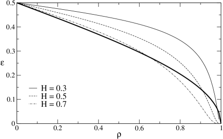
Abbildung 5.1: Probability of disagreeing hidden units in the case of queries with different parameter $H$ and $Q=1$. The thick line shows $P(\sigma_{i}^{A}\not=\sigma_{i}^{B})$ for random inputs.

As shown in figure 5.1 using queries affects the probability that two corresponding hidden units disagree on their output $\sigma_{i}$. Compared to the case of a random input sequence, this event occurs more frequently for small overlap, but less for nearly synchronized neural networks. Hence queries are especially a problem for the attacker. As learning is slower than synchronization, $\rho_{i}^{\mathrm{AE}}$ is typically smaller than $\rho_{i}^{\mathrm{AB}}$. In this situation queries increase the probability of repulsive steps for the attacker, while the partners are able to regulate this effect by choosing $H$ in a way that it does not interfere much with their process of synchronization. Consequently, using queries gives A and B more control over the difficulty of both synchronization and learning.

5.2 Synchronization time

Because queries change the relation between the overlap $\rho_{i}^{AB}$ and the probability of repulsive steps $P_{\mathrm{r}}^{B}(\rho_{i}^{AB})$, using them affects the number of steps needed to reach full synchronization. But the neural key-exchange protocol is only useful in practice, if the synchronization time $t_{\mathrm{sync}}$ is not too large. Otherwise, there is no advantage compared to classical algorithms based on number theory. This condition, of course, restricts the usable range of the new parameter $H$.

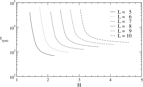
Abbildung 5.2: Synchronization time of two Tree Parity Machines with $K=3$, $N=1000$, and random walk learning rule, averaged over $10\,000$ simulations.

As shown in 5.2, $\langle t_{\mathrm{sync}}\rangle$ diverges for $H\rightarrow 0$. In this limit the prediction error $\epsilon^{\mathrm{p}}$ reaches $1/2$ independent of the overlap, so that the effect of the repulsive steps inhibits synchronization. But as long as $H$ is chosen large enough, it does not have much influence on the effort of generating a key [23].

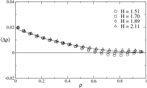
Abbildung 5.3: Average change of the overlap for synchronization with queries using $K=3$, $L=5$, $N=1000$, and the random walk learning rule. Symbols denote results obtained in $10\,000$ simulations, while the line shows $\langle\Delta\rho\rangle$ for synchronization with random inputs.

In fact, A and B can switch the mechanism of synchronization by modifying $H$. This is clearly visible in figure 5.3. If the absolute value of the local fields is so large that $\langle\Delta\rho\rangle>0$ for all $\rho<1$, synchronization on average happens, which is similar to the normal key-exchange protocol using a random sequence of input vectors. But decreasing $H$ below a certain value $H_{\mathrm{f}}$ creates a new fixed point of the dynamics at $\rho_{\mathrm{f}}<1$. In this case synchronization is only possible by fluctuations. As the gap with $\langle\Delta\rho\rangle<0$ grows with decreasing $H<H_{\mathrm{f}}$, one observes a steep increase of the average synchronization time $\langle t_{\mathrm{sync}}\rangle$. If A and B use the random walk learning rule together with $K=3$, $L=5$, and $N=1000$, one finds $H_{\mathrm{f}}\approx 1.76$ in this case.

Additionally, figure 5.2 shows a dependency on the synaptic depth $L$ of $\langle t_{\mathrm{sync}}\rangle$, which is caused by two effects [23]:

• The speed of synchronization is proportional to the step sizes $\langle\Delta\rho_{\mathrm{a}}\rangle$ for attractive and $\langle\Delta\rho_{\mathrm{r}}\rangle$ for repulsive steps. As shown in section 3.1.2, these quantities decrease proportional to $L^{-2}$. Therefore the average synchronization time increases proportional to the square of the synaptic depth as long as $H>H_{\mathrm{f}}$:

  $$\langle t_{\mathrm{sync}}\rangle\propto L^{2}\,.$$ (5.1)

  This causes the vertical shift of the curves in figure 5.2.

• If queries are used, the probabilities $P_{\mathrm{a}}$ for attractive and $P_{\mathrm{r}}$ for repulsive steps depend not only on the overlap $\rho_{i}$, but also on quantity $H/\sqrt{Q_{i}}$ according to (3.30). In the case of the random walk learning rule the weights stay uniformly distributed, so that the length of the weight vectors grows proportional to $L$ as shown in section 3.1.1. That is why one has to increase $H$ proportional to the synaptic depth,

  $$H=\alpha L\,,$$ (5.2)

  in order to achieve identical transition probabilities and consequently the same average synchronization time. This explains the horizontal shift of the curves in figure 5.2.

Using both scaling laws (5.1) and (5.2) one can rescale $\langle t_{\mathrm{sync}}\rangle$ in order to obtain functions $f_{L}(\alpha)$ which are nearly independent of the synaptic depth except for finite-size effects [23]:

$$\langle t_{\mathrm{sync}}\rangle=L^{2}f_{L}\!\left(\frac{H}{L}\right)\,.$$ (5.3)

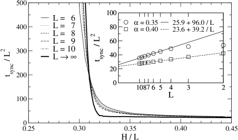
Abbildung 5.4: Scaling behavior of the synchronization time. The thick curve denotes the universal function $f(\alpha)$ defined in (5.4). It has been obtained by finite-size scaling, which is shown in the inset.

Figure 5.4 shows these functions for different values of $L$. It is clearly visible that $f_{L}(\alpha)$ converges to a universal scaling function $f(\alpha)$ in the limit $L\rightarrow\infty$:

$$f(\alpha)=\lim_{L\rightarrow\infty}f_{L}(\alpha)\,.$$ (5.4)

Additionally, the finite-size effects have a similar behavior in regard to $L$ as the fluctuations of the overlap $\rho_{i}$, which have been analyzed in section 3.4.2. That is why the distance $|f_{L}(\alpha)-f(\alpha)|$ shrinks proportional to $L^{-1}$. Therefore the universal function $f(\alpha)$ can be determined by finite-size scaling, which is shown in figure 5.4, too.

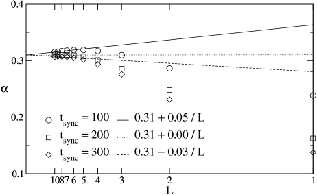
Abbildung 5.5: Extrapolation of the inverse function $f_{L}^{-1}$ to $L\rightarrow\infty$. Symbols denote the values extracted from figure 5.4 for different average synchronization times.

This function diverges for $\alpha<\alpha_{\mathrm{c}}$. The critical value $\alpha_{\mathrm{c}}=H_{\mathrm{c}}/L$ can be estimated by extrapolating the inverse function $f_{L}^{-1}$, which is shown in 5.5. By doing so one finds $\alpha_{\mathrm{c}}\approx 0.31$ for $K=3$ and $N=1000$, if A and B use the random walk learning rule [22]. Consequently, synchronization is only achievable for $H>\alpha_{\mathrm{c}}L$ in the limit $L\rightarrow\infty$. However, in the case of finite synaptic depth synchronization is even possible slightly below $H_{\mathrm{c}}$ due to fluctuations [23].

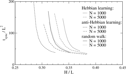
Abbildung 5.6: Synchronization time for neural cryptography with queries. These results have been obtained in $100$ simulations with $K=3$ and $L=7$.

Although the weights do not stay uniformly distributed in the case of Hebbian and anti-Hebbian learning, one observes qualitatively the same behavior of $\langle t_{\mathrm{sync}}\rangle$ as a function of the parameters $H$ and $L$. This is clearly visible in figure 5.6. As the length of the weight vectors is changed by these learning rules, the critical local field $H_{\mathrm{c}}=\alpha_{\mathrm{c}}L$ for synchronization is different. In the case of $K=3$ and $N=1000$, one finds $\alpha_{\mathrm{c}}\approx 0.36$ for Hebbian learning [23] and $\alpha_{\mathrm{c}}\approx 0.25$ for anti-Hebbian learning. But in the limit $N\rightarrow\infty$ the behavior of both learning rules converges to that of the random walk learning rule [22], which is also visible in figure 5.6.

5.3 Security against known attacks

Because of the cryptographic application of neural synchronization it is important that the key-exchange protocol using queries is not only efficient, but also secure against the attacks known up to now. Therefore it is necessary to determine how different absolute values of the local field influence the security of the system. Of course, the results impose further restrictions upon the usable range of the parameter $H$.

5.3.1 Dynamics of the overlap

Replacing random inputs with queries gives A and B an additional advantage over E. Now they can choose a suitable value of the new parameter $H$, which influences the probability of repulsive steps as shown in figure 5.1 (on page 5.1). By doing so the partners are able to modify the dynamics of the synchronization process, not only for themselves, but also for an attacker. And because $\langle\Delta\rho^{AB}(\rho)\rangle$ is greater than $\langle\Delta\rho^{AE}(\rho)\rangle$, A and B can generate queries in such a way that a fixed point of the dynamics at $\rho_{\mathrm{f}}<1$ only exists for E. Then the neural key-exchange protocol is secure in principle, because $\langle t_{\mathrm{sync}}^{E}\rangle$ grows exponentially with increasing synaptic depth while $\langle t_{\mathrm{sync}}^{B}\rangle\propto L^{2}$.

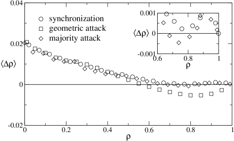
Abbildung 5.7: Average change of the overlap for $K=3$, $L=5$, $N=1000$, $H=1.77$, and $M=100$. Symbols denote results obtained in $200$ simulations using the random walk learning rule.

Figure 5.7 shows that this is indeed possible. Here A and B have chosen $H\approx H_{\mathrm{f}}$, so that they just synchronize on average. In contrast, E can reach the absorbing state at $\rho=1$ only by fluctuations, as there is a fixed point of the dynamics at $\rho_{\mathrm{f}}<1$ for both the geometric attack and the majority attack. In principle, this situation is similar to that observed in the case of random inputs. However, the gap between the fixed point and the absorbing state is larger, so that the success probability of both attacks is decreased. This is clearly visible by comparing figure 5.3 with figure 3.16 (on page 3.16) and figure 4.7 (on page 4.7).

5.3.2 Success probability

In practice it is necessary to look at the success probability $P_{E}$ of the known attacks in order to determine the level of security provided by neural cryptography with queries.

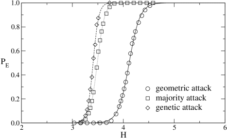
Abbildung 5.8: Success probability $P_{E}$ as a function of $H$. Symbols denote the results obtained in $1000$ simulations using $K=3$, $L=10$, $N=1000$, and the random walk learning rule, while the lines show fit results for model (5.5). The number of attacking networks is $M=4096$ for the genetic attack and $M=100$ for the majority attack.

As shown in figure 5.8, E is nearly always successful in the case of large $H$, because she is able to synchronize on average similar to A and B. But if $H$ is small, the attacker can reach full synchronization only by fluctuations, so that $P_{E}$ drops to zero. In fact, one can use a Fermi-Dirac distribution

$$P_{\mathrm{E}}=\frac{1}{1+\exp(-\beta(H-\mu))}$$ (5.5)

as a suitable fitting function in order to describe $P_{E}$ as a function of $H$. This model is suitable for both the majority attack [23] and the genetic attack [22]. Of course, one can also use it to describe $P_{E}(H)$ of the geometric attack, which is the special case $M=1$ of the more advanced attacks. Comparing these curves in figure 5.8 reveals directly that the genetic attack is the best choice for the attacker in this case.

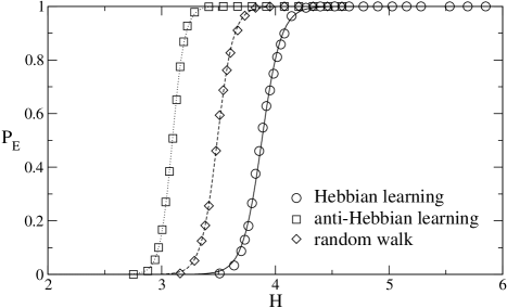
Abbildung 5.9: Success probability $P_{E}$ of the majority attack for $K=3$, $L=10$, $N=1000$, and $M=100$. Symbols denote results obtained in $10\,000$ simulations, while lines represents fits with model (5.5).

Additionally, one observes a similar behavior for all three learning rules. This is clearly visible in figure 5.9. Only the fit parameters are different due to the changed length of the weight vectors. Hebbian learning increases $Q_{i}$, so that an higher value of $H$ is needed in order to achieve the same value of the success probability. In contrast, the anti-Hebbian learning rule decreases $Q_{i}$, so that one observes a similar behavior with a lower value of $H$. Consequently, equation (5.5) is a universal model, which describes the success probability $P_{E}$ as a function of the absolute local field $H$ for all known attacks.

However, it is not sufficient to know the fit parameters $\mu$ and $\beta$ for only one value of the synaptic depth. In order to estimate the security of the neural key-exchange protocol with queries, one has to look at the scaling behavior of these quantities in regard to $L$.

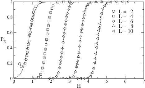
Abbildung 5.10: Success probability of the geometric attack for $K=3$, $N=1000$, and the Hebbian learning rule. Symbols denote results obtained in $10\,000$ simulations, while lines show fits with model (5.5).

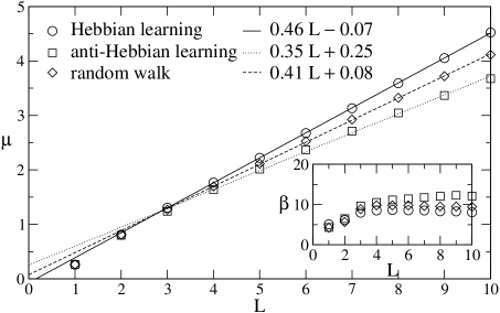
Abbildung 5.11: Parameters $\mu$ and $\beta$ as a function of the synaptic depth $L$ for the geometric attack. Symbols denote the results of fits using model (5.5), based on $10\,000$ simulations with $K=3$ and $N=1000$.

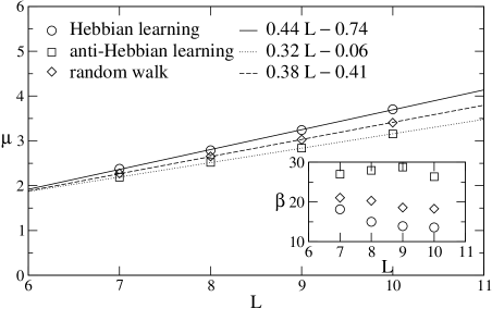
Abbildung 5.12: Parameter $\mu$ and $\beta$ as a function of $L$ for the genetic attack with $K=3$, $N=1000$, and $M=4096$. The symbols represent results from $1000$ simulations and the lines show a fit using the model given in (5.6).

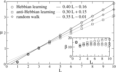
Abbildung 5.13: Parameters $\mu$ and $\beta$ as a function of the synaptic depth $L$ for the majority attack. Symbols denote the results of fits using model (5.5), based on $10\,000$ simulations with $K=3$, $N=1000$, and $M=100$.

Figure 5.10 shows that increasing the synaptic depth does not change the shape of $P_{E}(H)$ much, so that the steepness $\beta$ is nearly constant for $L>3$. But there is a horizontal shift of the curves due to the growing length of the weight vectors. In fact, the position $\mu$ of the smooth step increases linearly with the synaptic depth $L$,

$$\mu=\alpha_{\mathrm{s}}L+\delta\,,$$ (5.6)

which is shown in figure 5.11. As before, the method chosen by E does not matter, because equation (5.6) is valid in all cases [23, 22]. Only the parameters $\alpha_{\mathrm{s}}$ and $\delta$ depend on the learning rule and the attack. This is clearly visible in figure 5.12 and in figure 5.13.

Combining (5.5) and (5.6) yields

$$P_{\mathrm{E}}=\frac{1}{1+\exp(\beta\,\delta)\exp(\beta\,(\alpha_{\mathrm{s}}-\alpha)L)}$$ (5.7)

for the success probability of any known attack. As long as A and B choose $\alpha=H/L$ according to the condition $\alpha<\alpha_{\mathrm{s}}$, $P_{E}$ vanishes for $L\rightarrow\infty$. In this case its asymptotic behavior is given by

$$P_{\mathrm{E}}\sim\mathrm{e}^{-\beta\,\delta}\,\mathrm{e}^{-\beta\,(\alpha_{\mathrm{s}}-\alpha)L}\,,$$ (5.8)

which is consistent with the observation

$$P_{\mathrm{E}}\sim\mathrm{e}^{-y(L-L_{0})}$$ (5.9)

found for neural cryptography with random inputs [16]. Comparing the coefficients in both equations reveals

$$y = \beta\,(\alpha_{\mathrm{s}}-\alpha)\,,$$ (5.10)

$$L_{0} = -\delta/(\alpha_{\mathrm{s}}-\alpha)\,.$$ (5.11)

Thus replacing random inputs with queries gives A and B direct influence on the scaling of $P_{E}$ in regard to $L$, as they can change $y$ by modifying $\alpha$. Finally, the results indicate that there are two conditions for a fast and secure key-exchange protocol based on neural synchronization with queries:

• As shown in section 5.2 the average synchronization time $\langle t_{\mathrm{sync}}\rangle$ diverges in the limit $L\rightarrow\infty$, if $H$ is too small. Therefore A and B have to choose this parameter according to $H>\alpha_{\mathrm{c}}L$.

• And if $H$ is too large, the key-exchange becomes insecure, because $P_{E}=1$ is reached in the limit $L\rightarrow\infty$. So the partners have to fulfill the condition $H<\alpha_{\mathrm{s}}L$ for all known attacks.

Fortunately, A and B can always choose a fixed $\alpha=H/L$ according to

$$\alpha_{\mathrm{c}}<\alpha<\alpha_{\mathrm{s}}\,,$$ (5.12)

as there is no known attack with $\alpha_{\mathrm{s}}\leq\alpha_{\mathrm{c}}$. Then $\langle t_{\mathrm{sync}}\rangle$ grows proportional to $L^{2}$, but $P_{E}$ drops exponentially with increasing synaptic depth. Consequently, A and B can reach any desired level of security by just changing $L$ [22].

5.3.3 Optimal local field

For practical aspects of security, however, it is important to look at the relation between the average synchronization time and the success probability, as a too complex key-exchange protocol is nearly as unusable as an insecure one. That is why A and B want to minimize $P_{E}$ for a given value of $\langle t_{\mathrm{sync}}\rangle$ by choosing $L$ and $H$ appropriately. These optimum values can be determined by analyzing the function $P_{E}(\langle t_{\mathrm{sync}}\rangle)$.

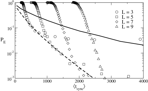
Abbildung 5.14: Success probability of the geometric attack as a function of $\langle t_{\mathrm{sync}}\rangle$. Symbols denote results obtained in $10\,000$ simulations using the Hebbian learning rule, $K=3$, and $N=1000$. The solid curve represents $P_{E}$ in the case of random inputs and the dashed line marks $H=0.36\,L$.

Figure 5.14 shows the result for the geometric attack. The optimum value of $H$ lies on the envelope of all functions $P_{\mathrm{E}}(\langle t_{\mathrm{sync}}\rangle)$. This curve is approximately given by $H=\alpha_{\mathrm{c}}L$, as this choice maximizes $\alpha_{\mathrm{s}}-\alpha$, while synchronization is still possible [23]. It is also clearly visible that queries improve the security of the neural key-exchange protocol greatly for a given average synchronization time.

Abbildung 5.15: Success probability of the majority attack as a function of $\langle t_{\mathrm{sync}}\rangle$. Symbols denote results obtained in $10\,000$ simulations using the Hebbian learning rule, $K=3$, $M=100$, and $N=1000$. The solid curve represents $P_{E}$ in the case of random inputs and the dashed line marks $H=0.36\,L$.

A similar result is obtained for the majority attack. Here figure 5.15 shows that the partners can even do better by using queries with $H<\alpha_{\mathrm{c}}L$ as long as $L$ is not too large. This effect is based on fluctuations which enable synchronization, but vanish in the limit $L\rightarrow\infty$. Thus the optimum value of $H$ is still given by $H\approx\alpha_{\mathrm{c}}L$ if $L\gg 1$. Additionally, figure 5.15 indicates that A and B can even employ the Hebbian learning rule for neural cryptography with queries, which led to an insecure key-exchange protocol in the case of random inputs [21, 23].

5.3.4 Genetic attack

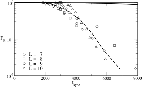
Abbildung 5.16: Success probability of the genetic attack as a function of $\langle t_{\mathrm{sync}}\rangle$. Symbols denote results obtained in $1000$ simulations using the random walk learning rule, $K=3$, $M=4096$, and $N=1000$. The solid curve represents $P_{E}$ in the case of random inputs and the dashed line marks $H=0.32\,L$.

Compared to the other methods the genetic attack is in a certain way different. First, it is especially successful, if $L$ is small. That is why A and B have to use Tree Parity Machines with large synaptic depth $L$ regardless of the parameter $H$. Of course, this sets a lower limit for the effort of performing the neural key-exchange protocol as shown in figure 5.16.

Second, the genetic attack is a rather complicated algorithm with a lot of parameters. Of course, E tries to optimize them in order to adapt to special situations. Here the number $M$ of attacking networks is clearly the most important parameter, because it limits the number of mutation steps $t_{\mathrm{s}}$ which can occur between two selection steps:

$$t_{\mathrm{s}}\leq\frac{1}{K-1}\frac{\ln M}{\ln 2}\,.$$ (5.13)

Thus E can test different variants of the internal representation $(\sigma_{1},\dots\sigma_{K})$ for at most $t_{\mathrm{s}}$ steps, before she has to select the fittest Tree Parity Machines. And more time results in better decisions eventually. Therefore one expects that E can improve $P_{E}$ by increasing $M$ similar to the effect observed for random inputs in section 4.1.2.

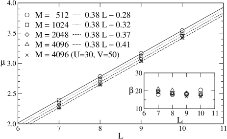
Abbildung 5.17: Parameter $\mu$ and $\beta$ as a function of $L$ for the genetic attack with $K=3$, $N=1000$, and the random walk learning rule. Symbols denote results of fitting simulation data with (5.5) and the lines were calculated using the model given in (5.6).

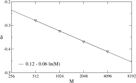
Abbildung 5.18: Offset $\delta$ as a function of the number of attackers $M$, for the genetic attack with $K=3$, $N=1000$, and the random walk learning rule. Symbols and the line were obtained by a fit with (5.14).

Figure 5.17 shows that this is indeed the case. While $\alpha_{\mathrm{s}}$ stays constant, the offset $\delta$ decreases with increasing $M$. As before, it is a logarithmic effect,

$$\delta(M)=\delta(1)-\delta_{E}\ln M\,,$$ (5.14)

which is clearly visible in figure 5.18. Therefore E gains a certain horizontal shift $\delta_{E}\ln 2$ of the smooth step function $P_{E}(H)$ by doubling the effort used for the genetic attack [22]. Combining (4.9) and (5.7) yields

$$P_{E}=\frac{1}{1+\exp(\beta(\delta(1)-\delta_{E}\ln M))\exp(\beta(\alpha_{s}-\alpha)L)}$$ (5.15)

for the success probability of this method. Then the asymptotic behavior for $L\gg 1$ is given by

$$P_{E}\sim e^{-\beta(\delta(1)-\delta_{E}\ln M)}e^{-\beta(\alpha_{s}-\alpha)L}$$ (5.16)

as long as $\alpha<\alpha_{\mathrm{s}}$. Similar to neural cryptography with random inputs E has to increase the number of attacking networks exponentially,

$$M\propto e^{[(\alpha_{s}-\alpha)/\delta_{E}]L}\,,$$ (5.17)

in order to maintain a constant success probability $P_{E}$, if A and B change the synaptic depth $L$. But, due to limited computer power, this is often not feasible.

Abbildung 5.19: Success probability of the genetic attack in the case of $K=3$, $L=7$, $N=1000$, $M=4096$, $H=2.28$, and random walk learning rule. These results were obtained by averaging over $100$ simulations.

However, the attacker could also try to improve $P_{E}$ by changing the other parameters $U$ and $V$ of the genetic attack. Instead of the default values $U=10$, $V=20$ E could use $U=30$, $V=50$, which maximize $P_{E}$ without greatly changing the complexity of the attack [22]. But this optimal choice, which is clearly visible in figure 5.19, does not help much as shown in figure 5.17. Only $\beta$ is lower for the optimized attack, while $\alpha_{\mathrm{s}}$ remains nearly the same. Therefore the attacker gains little, as the scaling relation (5.17) is not affected. Consequently, the neural key-exchange protocol with queries is even secure against an optimized variant of the genetic attack in the limit $L\rightarrow\infty$.

5.3.5 Comparison of the attacks

Of course, the opponent E always employs the best method, which is available to her in regard to computing power and other resources. Therefore it is necessary to compare all known attack methods in order to estimate the level of security achieved by a certain set of parameters.

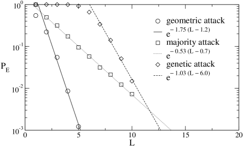
Abbildung 5.20: Success probability of different attacks as a function of the synaptic depth $L$. Symbols denote results obtained in $1000$ simulations using the random walk learning rule, $K=3$, $H=0.32L$, and $N=1000$, while the lines show fit results for model (5.9). Here E has used $M=4096$ networks for the genetic attack and $M=100$ for the majority attack.

The result for neural cryptography with queries is shown in figure 5.20. It is qualitatively similar to that observed in section 4.1.4 in the case of synchronization with random inputs. As the majority attack has the minimum value of $\alpha_{\mathrm{s}}$, it is usually the best method for the attacker. Only if A and B use Tree Parity Machines with small synaptic depth, the genetic attack is better.

However, comparing figure 5.20 with figure 4.9 (on page 4.9) reveals, that there are quite large quantitative differences, as replacing random inputs with queries greatly improves the security of the neural key-exchange protocol. Extrapolation of (5.9) shows that $P_{E}\approx 10^{-4}$ is achieved for $K=3$, $L=18$, $N=1000$, $H=5.76$, and random walk learning rule. This is much easier to realize than $L=57$, which would be necessary in order to reach the same level of security in the case of random inputs.

5.4 Possible security risks

Although using queries improves the security of the neural key-exchange protocol against known attacks, there is a risk that a clever attacker may improve the success probability $P_{E}$ by using additional information revealed through the algorithm generating the input vectors. Two obvious approaches are analyzed here. First, E could use her knowledge about the absolute local field $H$ to improve the geometric correction of the internal representation $(\sigma_{1}^{E},\dots,\sigma_{K}^{E})$. Second, each input vector $\mathbf{x}_{i}$ is somewhat correlated to the corresponding weight vector $\mathbf{w}_{i}$ of the generating network. This information could be used for a new attack method.

5.4.1 Known local field

If the partners use queries, the absolute value of the local field in either A’s or B’s hidden units is given by $H$. And E knows the local fields $h_{i}^{E}$ in her own Tree Parity Machine. In this situation the probability of $\sigma_{i}^{E}\not=\sigma_{i}^{A}$ is no longer given by (3.20) or (3.30), if it is A’s turn to generate the input vectors. Instead, one finds

$$P(\sigma_{i}^{E}\not=\sigma_{i}^{A})=\left[1+\exp\left(\frac{2\rho_{i}^{AE}}{1-(\rho_{i}^{AE})^{2}}\frac{H}{\sqrt{Q_{i}^{A}}}\frac{|h_{i}^{E}|}{\sqrt{Q_{i}^{E}}}\right)\right]^{-1}\,.$$ (5.18)

Although one might assume that this probability is minimal for $|h_{i}^{E}|\approx H$, it is not the case. In contrast, $P(\sigma_{i}^{E}\not=\sigma_{i}^{A})$ reaches its maximum at $|h_{i}^{E}|=0$ and is a strictly decreasing function of $|h_{i}^{E}|$ as before.

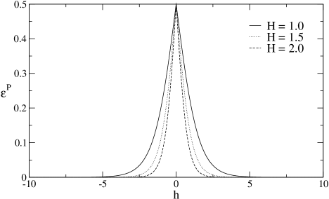
Abbildung 5.21: Prediction error $\epsilon_{i}^{\mathrm{p}}$ as a function of the local field $h_{i}^{E}$ for $Q_{i}^{A}=1$, $Q_{i}^{E}=1$, and $\rho=0.5$.

This is clearly visible in figure 5.21. As there is no qualitative difference compared to synchronization with random inputs, it is not possible to improve the geometric attack by using $H$ as additional information. Instead, it is still optimal for E to flip the output of that hidden unit, which has the minimum absolute value of the local field.

5.4.2 Information about weight vectors

While $H$ cannot be used directly in the geometric attack, queries give E additional information about the weight vectors in A’s and B’s Tree Parity Machines. But fortunately the absolute local field $H$ used for synchronization with queries is lower than the average value

$$\langle|h_{k}|\rangle=\sqrt{2Q_{i}/\pi}\approx 0.8\sqrt{Q_{i}}$$ (5.19)

observed for random inputs. Hence the overlap

$$\rho_{i,\mathrm{in}}=\frac{\mathbf{w}_{i}\cdot\mathbf{x}_{i}}{\sqrt{\mathbf{w}_{i}\cdot\mathbf{w}_{i}}\sqrt{\mathbf{x}_{i}\cdot\mathbf{x}_{i}}}=\frac{1}{\sqrt{N}}\frac{h_{i}}{\sqrt{Q_{i}}}$$ (5.20)

between input vector and weight vector is very small and converges to zero in the limit $N\rightarrow\infty$, although $H>0$. Consequently, $\mathbf{x}_{i}$ and $\mathbf{w}_{i}$ are nearly perpendicular to each other, so that the information revealed by queries is minimized [23].

In fact, for a given value of $H$ the number of weight vectors, which are consistent with a given query, is still exponentially large. As an example, there are $2.8\times 10^{129}$ possible weight vectors for a query with $H=10$, $L=10$, and $N=100$ [23]. Consequently, E cannot benefit from the information contained in the input vectors generated by A and B.

Kapitel 6 Conclusions and outlook

In this thesis the synchronization of neural networks by learning from each other has been analyzed and discussed. At a glance this effect looks like an extension of online learning to a series of examples generated by a time dependent rule. However, it turns out that neural synchronization is a more complicated dynamical process, so that new phenomena occur.

This is especially true for Tree Parity Machines, whereas synchronization is driven by stochastic attractive and repulsive forces. Because this process does not have a self-averaging order parameter, one has to take the whole distribution of the weights into account instead of using just the average value of the order parameter to determine the dynamics of the system. This can be done using direct simulations of the variables $w_{i,j}$ for finite $N$ or a iterative calculation of their probability distribution in the limit $N\rightarrow\infty$.

While one can use different learning rules both for bidirectional synchronization and unidirectional learning, they show similar behavior and converge to the random walk learning rule in the limit $N\rightarrow\infty$. So the deviations caused by Hebbian and anti-Hebbian learning are, in fact, finite-size effects, which become only relevant for $L\gg O(\sqrt{N})$.

In contrast, numerical simulations as well as iterative calculations show a phenomenon, which is significant even in very large systems: In the case of Tree Parity Machines learning by listening is much slower than mutual synchronization. This effect is caused by different possibilities of interaction. Two neural networks, which can influence each other, are able to omit steps, if they caused a repulsive effect. This is an advantage compared to a third Tree Parity Machine, which is trained using the examples produced by the other two and cannot select the most suitable input vectors for learning. Consequently, if interaction is only possible in one direction, the frequency of repulsive steps is higher than in the case of bidirectional communication.

Although the overlap $\rho$ is not a self-averaging quantity, one can describe neural synchronization as a random walk in $\rho$-space. Here the average step sizes $\langle\Delta\rho_{\mathrm{a}}\rangle$ and $\langle\Delta\rho_{\mathrm{r}}\rangle$ are the same for synchronization and learning. But the transition probabilities $P_{\mathrm{a}}(\rho)$ and $P_{\mathrm{r}}(\rho)$ depend on the type of interaction. As a result one can observe qualitative differences regarding the dynamics of the overlap. In the case of $K=3$ and bidirectional interaction the average change of the overlap $\langle\Delta\rho\rangle$ is strictly positive, so that synchronization by mutual learning happens on average. But for $K>3$ or unidirectional interaction the higher probability of repulsive steps causes a fixed point of the dynamics at $\rho_{\mathrm{f}}<1$. Then reaching the absorbing state at $\rho=1$ is only possible by means of fluctuations.

While both mechanisms lead to full synchronization eventually, one observes two different distributions of the synchronization time depending on the function $\langle\Delta\rho(\rho)\rangle$. In the case of synchronization on average, it is a Gumbel distribution, because one has to wait until the last weight has synchronized. Analytical calculations for systems without repulsive steps yield the result $\langle t_{\mathrm{sync}}\rangle\propto L^{2}\ln N$. And a few repulsive steps do not change this scaling behavior, but simply increase the constant of proportionality.

In contrast, if synchronization is only possible by means of fluctuations, there is a constant probability per step to get over the gap with $\langle\Delta\rho(\rho)\rangle<0$ between the fixed point and the absorbing state. Of course, this yields an exponential distribution of the synchronization time. However, the fluctuations of the overlap in the steady state decrease proportional to $L^{-1}$. As they are essential for reaching $\rho=1$ in this case, the synchronization time grows exponentially with increasing synaptic depth of the Tree Parity Machines.

Without this difference a secure key-exchange protocol based on the synchronization of neural networks would be impossible. But as A’s and B’s Tree Parity Machines indeed synchronize faster than E’s neural networks, the partners can use the synchronized weight vectors as a secret session key. Of course, there is a small probability $P_{E}$ that E is successful before A and B have finished their key exchange due to the stochastic nature of the synchronization process. But fortunately $P_{E}$ drops exponentially with increasing $L$ for nearly all combinations of learning rules and attack methods. Thus A and B can achieve any level of security by just increasing the synaptic depth $L$.

Additionally, there are other observations which indicate that bidirectional interaction is an advantage for A and B compared to a passive attacker E. For a time series generated by two Tree Parity Machines the version space of compatible initial conditions is larger, if both are already synchronized at the beginning, than if the neural networks start unsynchronized. So it is harder for an attacker to imitate B because of the interaction between the partners. And, of course, the attack methods are unable to extract all the information which is necessary to achieve full synchronization. This effect is mainly caused by the fact, that A and B can choose the most useful input vectors from the random sequence, but E does not have this ability [45].

Thus the partners can improve the security of neural cryptography further, if they use a more advanced algorithm to select the input vectors. This approach eventually leads to synchronization with queries. In this variant of the key-exchange protocol A and B ask each other questions, which depend on the weights in their own networks. In doing so they are able to choose the absolute value of the local field in the Tree Parity Machine generating the current query. Of course, this affects both synchronization and attacks. However, E is at a disadvantage compared to A and B, because she needs a higher absolute value of the local field than the partners in order to synchronize on average. Therefore it is possible to adjust the new parameter $H$ in such a way, that A and B synchronize fast, but E is not successful regardless of the attack method.

However, the algorithm generating the input vectors does not matter for the opponent. E has no influence on it and the relative efficiency of the attacks stays the same, whether a random input sequence or queries are used. In both cases the majority attack is the best method as long as the synaptic depth is large. Only if $L$ is small, the genetic attack is better. Of course, both advanced attacks are always more successful than the geometric attack. And the simple attack is only useful for $K\gg 3$.

In any case, the effort of the partners grows only polynomially, while the success probability of an attack drops exponentially, if the synaptic depth increases. Similar scaling laws can be found, if one looks at other cryptographic systems. Only the parameter is different. While the security of conventional cryptography [26, 25] depends on the length of the key, the synaptic depth of the Tree Parity Machines plays the same role in the case of neural cryptography [22].

Brute-force attacks are not very successful, either. Here the number of keys grows exponentially with the system size $N$, while the synchronization time is only proportional to $\log N$. Thus A and B can use large systems without much additional effort in order to prevent successful guessing of the generated key.

Consequently, the neural key-exchange protocol is secure against all attacks known up to now. However, there is always the risk that one might find a clever attack, which breaks the security of neural cryptography completely, because it is hardly ever possible to prove the security of such an algorithm [25].

However, the neural key-exchange protocol is different from conventional cryptographic algorithms in one aspect. Here effects in a physical system, namely attractive and repulsive stochastic forces, are used instead of those found in number theory. In fact, the trap door function is realized by a dynamics, which is different for partners and attackers based on their possibilities of interaction with the other participants. Of course, neural networks are not the only type of systems with these properties. Any other system showing similar effects can be used for such a cryptographic application, too.

Interesting systems include chaotic maps and coupled lasers [46, 47, 48, 49]. In both cases one observes that synchronization is achieved faster for bidirectional than for unidirectional coupling. As this underlying effect is very similar, one can use nearly the same cryptographic protocol by just substituting the neural networks. Of course, this applies to the attack methods, too. For example, the algorithms of the majority attack and the genetic attack are so general, that they are also useful methods for attacks on key-exchange protocols using chaotic maps. In contrast, the geometric correction algorithm is rather specific for neural networks, so that it has to be replaced by appropriate methods.

Consequently, the neural key-exchange protocol is only the first element of a class of new cryptographic algorithms. Of course, all these proposals have to be analyzed in regard to efficiency and security. For that purpose the methods used in this thesis can probably act as a guidance. Especially synchronization by fluctuations and synchronization on average are rather abstract concepts, so that one should be able to observe them in a lot of systems.

Another interesting direction is the implementation of the neural key-exchange protocol. Computer scientists are already working on a hardware realization of interacting Tree Parity Machines for cryptographic purposes [50, 51, 52, 53, 54, 55]. They have especially found out that neural synchronization only needs very basic mathematical operations and, therefore, is very fast compared to algorithms based on number theory. Consequently, one can use neural cryptography in small embedded systems, which are unable to use RSA or other established methods [26, 25]. Here it does not matter that the neural key-exchange protocol only reaches a moderate level of security as long as one requires a small synchronization time. But integrated circuits can achieve a very high frequency of key updates, which compensates this disadvantage [50, 51, 52].

Finally, these approaches indicate that further development of neural cryptography is indeed possible. As mentioned before, there are, in fact, two distinct directions: First, one can extend the neural key-exchange protocol in order to improve the efficiency, security and usefulness for specific cryptographic applications, e. g. embedded systems. Second, one can replace the neural networks by other physical systems, e. g. chaotic lasers, which have similar properties to those identified in this thesis as essential for security.

Anhang A Notation

A	sender
B	receiver
E	attacker
$K$	number of hidden units in a Tree Parity Machine
$L$	synaptic depth of the neural networks
$N$	number of neurons per hidden unit
$M$	(maximum) number of attacking networks
$H$	absolute set value of the local field
$R$	threshold for the reset of the input vectors
$U$	minimal fitness
$V$	length of the output history
$\mathbf{w}_{i}$	weight vector of the $i$-th hidden unit
$\mathbf{x}_{i}$	input vector of the $i$-th hidden unit
$w_{i,j}$	$j$-th element of $\mathbf{w}_{i}$
$x_{i,j}$	$j$-th element of $\mathbf{x}_{i}$
$\sigma_{i}$	output of the $i$-th hidden unit
$\tau$	total output of a Tree Parity Machine
$h_{i}$	local field of the $i$-th hidden unit
$\rho_{i}$	overlap of the $i$-th hidden unit
$\epsilon_{i}$	generalization error
$\epsilon_{i}^{\mathrm{p}}$	prediction error
$P_{\mathrm{a}}$	probability of attractive steps
$P_{\mathrm{r}}$	probability of repulsive steps
$\Delta\rho_{\mathrm{a}}$	step size of an attractive step
$\Delta\rho_{\mathrm{r}}$	step size of a repulsive step
$\langle\Delta\rho\rangle$	average change of the overlap
$\rho_{\mathrm{f}}$	fixed point of the dynamics
$\sigma_{\mathrm{f}}$	width of the $\rho$-distribution at the fixed point
$I$	mutual information
$S$	entropy of a weight distribution
$S_{0}$	maximal entropy of a single neural network
$n_{\mathrm{conf}}$	number of possible weight configurations
$n_{\mathrm{key}}$	number of distinct keys
$n_{\mathrm{vs}}$	size of the version space
$T$	synchronization time for two random walks
$T_{N}$	synchronization time for $N$ pairs of random walks
$t_{\mathrm{sync}}$	synchronization time for two Tree Parity Machines
$P_{E}$	success probability of an attacker
$y$	sensitivity of $P_{E}$ in regard to $L$
$L_{0}$	minimal value of $L$ for the exponential decay of $P_{E}$
$\alpha$	rescaled local field $H/L$
$\alpha_{\mathrm{c}}$	minimum $\alpha$ for synchronization
$\alpha_{\mathrm{s}}$	maximum $\alpha$ for security
$\beta$	sensitivity of $P_{E}$ in regard to $H$
$\delta$	offset of $P_{E}(H)$
$\gamma$	Euler-Mascheroni constant ($\gamma\approx 0.577$)

Auxiliary functions for the learning rules

• control signal

  $$f(\sigma,\tau^{A},\tau^{B})=\Theta(\sigma\tau^{A})\Theta(\tau^{A}\tau^{B})\left\{\begin{array}[]{cl}\sigma&\mbox{ Hebbian learning rule }\\ -\sigma&\mbox{ anti-Hebbian learning rule }\\ 1&\mbox{ random walk learning rule }\end{array}\right.$$

• boundary condition

  $$g(w)=\left\{\begin{array}[]{cl}\mathrm{sgn}(w)\,L&\mbox{ for $|w|>L$ }\\ w&\mbox{ otherwise }\\ \end{array}\right.$$

Anhang B Iterative calculation

This appendix presents the algorithm, which is used to calculate the time evolution of the weight distribution iteratively in the limit $N\rightarrow\infty$ [18, 17, 19]. Compared to direct simulations $N$ weights are replaced by $(2L+1)\times(2L+1)$ variables $p^{i}_{a,b}$, which describe the probability that one finds a weight with $w_{i,j}^{A}=a$ and $w_{i,j}^{B}=b$. Consequently, one has to adapt both the calculation of the output bits and the update of the weight configuration.

B.1 Local field and output bits

According to its definition (2.3) the local field $h_{i}$ of a hidden unit is proportional to the sum over $N$ independent random variables $w_{i,j}\,x_{i,j}$. Therefore the central limit theorem applies and the probability to find certain values of $h_{i}^{A}$ and $h_{i}^{B}$ in a time step is given by

$$P(h_{i}^{A},h_{i}^{B})=\frac{e^{-(1/2)(h_{i}^{A},h_{i}^{B})\mathcal{C}_{i}^{-1}(h_{i}^{A},h_{i}^{B})^{T}}}{2\pi\sqrt{\det\mathcal{C}_{i}}}\,.$$ (B.1)

In this equation the covariance matrix $\mathcal{C}$ describes the correlations between A’s and B’s Tree Parity Machines in terms of the well-known order parameters $Q$ and $R$, which are functions of the weight distribution according to (2.11), (2.12), and (2.13):

$$\mathcal{C}_{k}=\left(\begin{array}[]{cc}Q_{i}^{A}&R_{i}^{AB}\\ R_{i}^{AB}&Q_{k}^{B}\end{array}\right)\,.$$ (B.2)

In order to generate local fields $h_{i}^{A}$ and $h_{i}^{B}$, which have the correct joint probability distribution (B.1), the following algorithm is used. A pseudo-random number generator produces two independent uniformly distributed random numbers $z_{1},z_{2}\in[0,1[$. Then the local fields are given by [56]

$$h_{i}^{A} = \sqrt{-2Q_{i}^{A}\ln(z_{1})}\cos(2\pi z_{2})\,,$$ (B.3)

$$h_{i}^{B} = \sqrt{-2Q_{i}^{B}\ln(z_{1})}\left[\rho\cos(2\pi z_{2})+\sqrt{1-\rho^{2}}\sin(2\pi z_{2})\right]\,.$$ (B.4)

Afterwards one can calculate the outputs $\sigma_{i}$ and $\tau$ in the same way as in the case of direct simulations. As the local fields are known, it is possible to implement the geometric correction, too. Therefore this method is also suitable to study synchronization by unidirectional learning, e. g. for a geometric attacker. Additionally, the algorithm can be extended to three and more interacting Tree Parity Machines [19].

B.2 Equations of motion

The equations of motion are generally independent of the learning rule, because the behavior of Hebbian and anti-Hebbian learning converges to that of the random walk learning rule in the limit $N\rightarrow\infty$. Consequently, the weights in both participating Tree Parity Machines stay uniformly distributed, only the correlations between $\mathbf{w}_{i}^{A}$ and $\mathbf{w}_{i}^{B}$ change.

Attractive steps

In an attractive step corresponding weights move in the same direction. Thus the distribution of the weights changes according to the following equations of motion for $-L<a,b<L$:

$$p^{i+}_{a,b} = \frac{1}{2}\left(p^{i}_{a+1,b+1}+p^{i}_{a-1,b-1}\right)\,,$$ (B.5)

$$p^{i+}_{a,L} = \frac{1}{2}\left(p^{i}_{a-1,L}+p^{i}_{a-1,L-1}\right)\,,$$ (B.6)

$$p^{i+}_{a,-L} = \frac{1}{2}\left(p^{i}_{a+1,-L}+p^{i}_{a+1,-L+1}\right)\,,$$ (B.7)

$$p^{i+}_{L,b} = \frac{1}{2}\left(p^{i}_{L,b-1}+p^{i}_{L-1,b-1}\right)\,,$$ (B.8)

$$p^{i+}_{-L,b} = \frac{1}{2}\left(p^{i}_{-L,b+1}+p^{i}_{-L+1,b+1}\right)\,,$$ (B.9)

$$p^{i+}_{L,L} = \frac{1}{2}\left(p^{i}_{L-1,L-1}+p^{i}_{L-1,L}+p^{i}_{L,L-1}+p^{i}_{L,L}\right)\,,$$ (B.10)

$$p^{i+}_{-L,-L} = \frac{1}{2}\left(p^{i}_{-L+1,-L+1}+p^{i}_{-L+1,-L}+p^{i}_{-L,-L+1}+p^{i}_{-L,-L}\right)\,,$$ (B.11)

$$p^{i+}_{L,-L} = 0\,,$$ (B.12)

$$p^{i+}_{-L,L} = 0\,.$$ (B.13)

Repulsive steps

In a repulsive step only the weights in one hidden unit move, either in A’s or in B’s Tree Parity Machine. However, the active hidden unit is selected randomly by the output bits, so that both possibilities occur with equal probability. Thus one can combine them in one set of equations for $-L<a,b<L$:

$$p^{i+}_{a,b} = \frac{1}{4}\left(p^{i}_{a+1,b}+p^{i}_{a-1,b}+p^{i}_{a,b+1}+p^{i}_{a,b-1}\right)\,,$$ (B.14)

$$p^{i+}_{a,L} = \frac{1}{4}\left(p^{i}_{a+1,L}+p^{i}_{a-1,L}+p^{i}_{a,L}+p^{i}_{a,L-1}\right)\,,$$ (B.15)

$$p^{i+}_{a,-L} = \frac{1}{4}\left(p^{i}_{a+1,-L}+p^{i}_{a-1,-L}+p^{i}_{a,-L+1}+p^{i}_{a,-L}\right)\,,$$ (B.16)

$$p^{i+}_{L,b} = \frac{1}{4}\left(p^{i}_{L,b}+p^{i}_{L-1,b}+p^{i}_{L,b+1}+p^{i}_{L,b-1}\right)\,,$$ (B.17)

$$p^{i+}_{-L,b} = \frac{1}{4}\left(p^{i}_{-L+1,b}+p^{i}_{-L,b}+p^{i}_{-L,b+1}+p^{i}_{-L,b-1}\right)\,,$$ (B.18)

$$p^{i+}_{L,L} = \frac{1}{4}\left(2p^{i}_{L,L}+p^{i}_{L-1,L}+p^{i}_{L,L-1}\right)\,,$$ (B.19)

$$p^{i+}_{-L,-L} = \frac{1}{4}\left(2p^{i}_{-L,-L}+p^{i}_{-L+1,-L}+p^{i}_{-L,-L+1}\right)\,,$$ (B.20)

$$p^{i+}_{L,-L} = \frac{1}{4}\left(2p^{i}_{L,-L}+p^{i}_{L-1,-L}+p^{i}_{L,-L+1}\right)\,,$$ (B.21)

$$p^{i+}_{-L,L} = \frac{1}{4}\left(2p^{i}_{-L,L}+p^{i}_{-L+1,L}+p^{i}_{-L,L-1}\right)\,.$$ (B.22)

Inverse attractive steps

Inverse attractive steps are only possible if A and B do not interact at all, but use common input vectors. In such a step corresponding weights move in the opposite direction. Thus the distribution of the weights changes according to the following equations of motion for $-L<a,b<L$:

$$p^{i+}_{a,b} = \frac{1}{2}\left(p^{i}_{a+1,b-1}+p^{i}_{a-1,b+1}\right)\,,$$ (B.23)

$$p^{i+}_{a,L} = \frac{1}{2}\left(p^{i}_{a+1,L}+p^{i}_{a+1,L-1}\right)\,,$$ (B.24)

$$p^{i+}_{a,-L} = \frac{1}{2}\left(p^{i}_{a-1,-L}+p^{i}_{a-1,-L+1}\right)\,,$$ (B.25)

$$p^{i+}_{L,b} = \frac{1}{2}\left(p^{i}_{L,b+1}+p^{i}_{L-1,b+1}\right)\,,$$ (B.26)

$$p^{i+}_{-L,b} = \frac{1}{2}\left(p^{i}_{-L,b-1}+p^{i}_{-L+1,b-1}\right)\,,$$ (B.27)

$$p^{i+}_{L,L} = 0\,,$$ (B.28)

$$p^{i+}_{-L,-L} = 0\,,$$ (B.29)

$$p^{i+}_{L,-L} = \frac{1}{2}\left(p^{i}_{L-1,-L+1}+p^{i}_{L-1,-L}+p^{i}_{L,-L+1}+p^{i}_{L,-L}\right)\,,$$ (B.30)

$$p^{i+}_{-L,L} = \frac{1}{2}\left(p^{i}_{-L+1,L-1}+p^{i}_{-L+1,L}+p^{i}_{-L,L-1}+p^{i}_{-L,L}\right)\,.$$ (B.31)

Anhang C Generation of queries

This appendix describes the algorithm [23] used to generate a query $\mathbf{x}_{i}$, which results in a previously chosen local field $h_{i}$. Finding an exact solution is similar to the knapsack problem [57] and can be very difficult depending on the parameters. Hence this is not useful for simulations, as one has to generate a huge number of input vectors $\mathbf{x}_{i}$ in this case. Instead a fast algorithm is employed, which gives an approximate solution.

As both inputs $x_{i,j}$ and weights $w_{i,j}$ are discrete, there are only $2L+1$ possible results for the product $w_{i,j}\,x_{i,j}$. Therefore a set of input vectors consisting of all permutations, which do not change $h_{i}$, can be described by counting the number $c_{i,l}$ of products with $w_{i,j}\,x_{i,j}=l$. Then the local field is given by

$$h_{i}=\frac{1}{\sqrt{N}}\sum_{l=1}^{L}l(c_{i,l}-c_{i,-l})\,,$$ (C.1)

which depends on both inputs and weights. But the sum $n_{i,l}=c_{i,l}+c_{i,-l}$ is equal to the number of weights with $|w_{i,j}|=|l|$ and thus independent of $\mathbf{x}_{i}$. Consequently, one can write $h_{i}$ as a function of only $L$ variables,

$$h_{i}=\frac{1}{\sqrt{N}}\sum_{l=1}^{L}l(2c_{i,l}-n_{i,l})\,,$$ (C.2)

as the values of $n_{i,l}$ are defined by the current weight vector $\mathbf{w}_{i}$.

In the simulations the following algorithm [23] is used to generate the queries. First the output $\sigma_{i}$ of the hidden unit is chosen randomly, so that the set value of the local field is given by $h_{i}=\sigma_{i}H$. Then the values of $c_{i,L}$, $c_{i,L-1}$, …, $c_{i,1}$ are calculated successively. For that purpose one of the following equations is selected randomly with equal probability, either

$$c_{i,l}=\left\lfloor\frac{n_{i,l}+1}{2}+\frac{1}{2l}\left(\sigma_{i}H\sqrt{N}-\sum_{j=l+1}^{L}j(2c_{i,j}-n_{i,j})\right)\right\rfloor$$ (C.3)

or

$$c_{i,l}=\left\lceil\frac{n_{i,l}-1}{2}+\frac{1}{2l}\left(\sigma_{i}H\sqrt{N}-\sum_{j=l+1}^{L}j(2c_{i,j}-n_{i,j})\right)\right\rceil\,,$$ (C.4)

in order to reduce the influence of rounding errors. Additionally, one has to take the condition $0\leq c_{i,l}\leq n_{i,l}$ into account. If equation (C.3) or equation (C.4) yield a result outside this range, $c_{i,l}$ is reset to the nearest boundary value.

Afterwards the input vector $\mathbf{w}_{i}$ is generated. Those $x_{i,j}$ associated with zero weights $w_{i,j}=0$ do not influence the local field, so that their value is just chosen randomly. But the other input bits $x_{i,j}$ are divided into $L$ groups according to the absolute value $l=|w_{i,j}|$ of their corresponding weight. Then $c_{i,l}$ input bits are selected randomly in each group and set to $x_{i,j}=\mathrm{sgn}(w_{i,j})$, while the other $n_{k,l}-c_{k,l}$ inputs are set to $x_{i,j}=-\mathrm{sgn}(w_{i,j})$.

Simulations show that queries generated by this algorithm result in local fields $h_{i}$ which match the set value $\sigma_{i}H$ on average [23]. Additionally, only very small deviations are observed, which are caused by the restriction of inputs and weights to discrete values. So this algorithm is indeed suitable for the generation of queries.