Homogenization of spectral problems
in bounded domains with doubly high contrasts

Abstract.

Homogenization of a spectral problem in a bounded domain with a high contrast in both stiffness and density is considered. For a special critical scaling, two-scale asymptotic expansions for eigenvalues and eigenfunctions are constructed. Two-scale limit equations are derived and relate to certain non-standard self-adjoint operators. In particular they explicitly display the first two terms in the asymptotic expansion for the eigenvalues, with a surprising bound for the error of order $\varepsilon^{5/4}$ proved.

2000 Mathematics Subject Classification. Primary: 35B27; Secondary: 34E

Key words. Homogenization, periodic media, high-contrasts, eigenvalue asymptotics

1. Introduction

Homogenization for problems with physical properties which are not only highly oscillatory but also highly heterogeneous has long been documented to display unusual effects, for example the memory effects observed by E. Ya. Khruslov [9, 13, 14]. Of particular interest in this context are the double-porosity models where the parameter of high-contrast $\delta$ is critically scaled again the periodicity size $\varepsilon$, $\delta\sim\varepsilon^{2}$, e.g. [2, 4]. Those have been treated both by a high-contrast version of the classical method of asymptotic expansions, e.g. [16, 17, 7, 12] and using the techniques of two-scale convergence, e.g. [19, 20, 5]. In particular, for spectral problems in bounded [19] and unbounded [20] periodic domains V.V. Zhikov studied the spectral convergence, introduced two-scale limit operator, developed the techniques of two-scale resolvent convergence and two-scale compactness. In [12] the spectral convergence of eigenvalues in the gaps of Floquet-Bloch spectrum due to defects in double-porosity type media were studied, and [5] supplemented this by the analysis of eigenfunction convergence based on an analysis of a uniform exponential decay.

In this work we study spectral problems of double-porosity type in a bounded domain $\Omega$ where the high contrast might occur not only in the “stiffness” coefficient but also in the “density”, and argue that this leads to some interesting new effects. Namely, referring to the next section for precise technical formulations, for the spectral problem

(1) $$-\,\mbox{div}\,(a_{\varepsilon}\left({x}\right)\nabla u_{\varepsilon})\,=\,\lambda^{\varepsilon}\rho_{\varepsilon}\left({x}\right)u_{\varepsilon},$$

with Dirichlet boundary conditions on the exterior boundary, most generally, both $a_{\varepsilon}$ and $\rho_{\varepsilon}$ are $\varepsilon$-periodic, $a_{\varepsilon}=\rho_{\varepsilon}=1$ in the connected matrix and $a_{\varepsilon}\sim\varepsilon^{\alpha}$, $\rho_{\varepsilon}\sim\varepsilon^{\beta}$ in the disconnected inclusions. (Outside homogenization, the above resembles problems of vibrations with high contrasts in both density and stiffness, e.g. [3].) The double-porosity corresponds to $\alpha=2$ and $\beta=0$. For $\beta\neq 0$, it is not hard to see that it is $\alpha=\beta+2$ when the spectral problems at the macro and micro-scales are coupled in a non-trivial way. To explore this, we choose $\beta=-1$ and $\alpha=1$ and show that this leads to some unusually coupled two-scale limit behaviors of the eigenfunctions and the eigenvalues.

Namely, although the limit behavior of the eigenfunctions is still somewhat similar to that of double porosity, i.e. the two-scale limit is a function of only slow variable $x$ in the matrix and a function of both $x$ and the fast variable $y$ in the inclusions, the limit equations themselves are quite different. We show that there exist asymptotic series of eigenvalues $\lambda^{\varepsilon}\sim\lambda_{0}+\varepsilon\lambda_{1}$ with $\lambda_{0}$ being any eigenvalue of a non-standard self-adjoint “microscopic” inclusion problem, Theorem 3.1, whose eigenfunctions are directly related to the two-scale limit $w_{0}(x,y)$ in the matrix. In fact, $\lambda_{0}$ is either a solution of $\beta(\lambda_{0})=|Q_{1}|\lambda_{0}$, where $\beta(\lambda)$ is a function introduced by Zhikov [19], or is an eigenvalue of the Dirichlet Laplacian in the inclusion $Q_{0}$ with a zero mean eigenfunction. In the matrix, $u_{\varepsilon}\sim v^{0}(x)$, where $v^{0}$ is an eigenfunction of the homogenized operator in $\Omega$, whose eigenvalue $\nu$ determines the second term $\lambda_{1}$ in the asymptotics of $\lambda^{\varepsilon}$, see (59). This is first derived via formal asymptotic expansions, but then we prove a non-standard error bound:

$$|\lambda^{\varepsilon}-\lambda_{0}-\varepsilon\lambda_{1}|\leq C\varepsilon^{5/4},$$

see Theorems 4.6 & 4.7. The proof employs a combination of a high contrast boundary layer analysis with maximum principle and estimates in Hilbert spaces with $\varepsilon$-dependent weights. We finally briefly discuss further refinement of the results via the technique of two-scale convergence. Namely, some version of the compactness result holds, cf. [19], indicating at the presence of gaps in the spectrum for small enough $\varepsilon$, see Theorem 5.1.

The paper is organized as follows. The next section formulates the problem and introduces necessary notation, Section 3 executes formal asymptotic expansion and derives associated homogenized equations. Section 4 proves the error bounds and Section 5 discusses the two-scale convergence approach. Some technical details are assembled in the appendices.

2. Problem statement and notations

We consider a model of eigenvibrations for a body occupying a bounded domain $\Omega$ in $\mathbb{R}^{n}$ ($n=2,3,\dots$) containing a periodic array of small inclusions, see Figure 1. The size of inclusions is controlled by a small positive parameter $\varepsilon$, $\varepsilon\to 0$. First we introduce necessary notation.

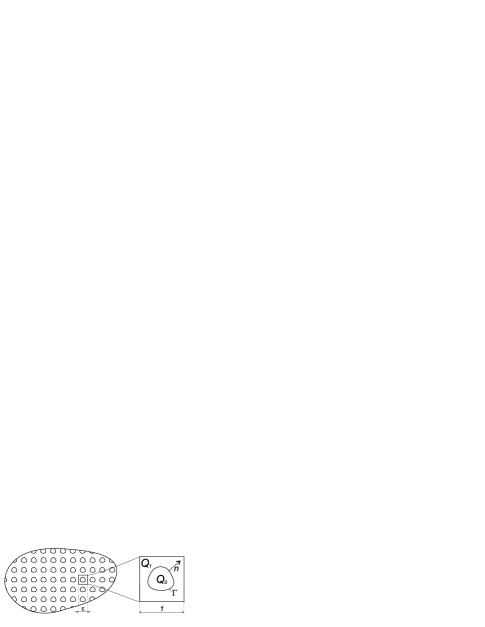
Figure 1. The geometry and the periodicity cell

Let $Q=[0,1]^{n}$ be a reference periodicity cell in $\mathbb{R}^{n}$. Let $\widetilde{Q}_{0}$ be a periodic set of “inclusions”, i.e. $\widetilde{Q}_{0}+m=\widetilde{Q}_{0}$, $\forall m\in\mathbb{Z}^{n}$, and $Q_{0}=\widetilde{Q}_{0}\cap Q$ is a reference inclusion lying inside $Q$ with $C^{2}$-smooth boundary $\Gamma$, see Figure 1. Let $Q_{1}=Q\backslash\overline{Q_{0}}$, $\widetilde{Q}_{1}=\mathbb{R}^{n}\backslash\overline{\widetilde{Q}_{0}}$, $\widetilde{\Gamma}=\partial\widetilde{Q}_{0}=\partial\widetilde{Q}_{1}$. Introducing $y=x/\varepsilon$ we refer to $y$ as to a fast variable, as opposes to the slow variable $x$. In the $x$-variable the periodicity cell is $\varepsilon Q=[0,\varepsilon)^{n}$. If $y\in Q_{j}$ then $x=\varepsilon y\in\varepsilon Q_{j}$, $j=0,1$. We denote $\Omega_{0}^{\varepsilon}:=\Omega\cap\varepsilon\tilde{Q}_{0}$, $\Omega_{1}^{\varepsilon}:=\Omega\cap\varepsilon\tilde{Q}_{1}=\Omega\backslash\overline{\Omega_{0}^{\varepsilon}}$, $\Gamma^{\varepsilon}:=\varepsilon\tilde{\Gamma}\cap\Omega$, see Figure 1. The trace on ${\Gamma}^{\varepsilon}$ of function $f:\Omega_{j}^{\varepsilon}\to\mathbb{R}^{n}$ is denoted by $f|_{j}$. Let $n_{y}$ be the outer unit normal to $Q_{0}$ on its boundary $\Gamma$ and let $n_{x}$ denote the similar normal on ${\Gamma}^{\varepsilon}$.

Let stiffness $a_{\varepsilon}$ and density $\rho_{\varepsilon}$ be as follows

$$a_{\varepsilon}\left({x}\right)=\left\{\begin{array}[]{rl}1,&x\in\Omega_{1}^{\varepsilon}\\ \varepsilon,&x\in\Omega_{0}^{\varepsilon}\end{array}\right.\quad\mbox{and}\quad\rho_{\varepsilon}\left({x}\right)=\left\{\begin{array}[]{rl}1,&x\in\Omega_{1}^{\varepsilon}\\ \varepsilon^{-1},&x\in\Omega_{0}^{\varepsilon}\end{array}\right.$$

with a small positive $\varepsilon$.

We study the asymptotic behaviour of self-adjoint spectral problem

(2) $$\int_{\Omega}a_{\varepsilon}\left({x}\right)\nabla u_{\varepsilon}\nabla\phi\,dx-\lambda^{\varepsilon}\int_{\Omega}\rho_{\varepsilon}\left({x}\right)u_{\varepsilon}\phi\,dx=0,\quad\forall\phi\in H^{1}_{0}(\Omega)$$

as $\varepsilon\to 0$. If $\Gamma$ and $\partial\Omega$ are smooth enough then variational problem (2) can be equivalently represented in a classical formulation

(3) $$-\,\mbox{div}\,(a_{\varepsilon}\left({x}\right)\nabla u_{\varepsilon}) = \lambda^{\varepsilon}\rho_{\varepsilon}\left({x}\right)u_{\varepsilon},\quad x\in\Omega,$$

(4) $$u_{\varepsilon}|_{\partial\Omega} = 0,$$

implying that at the interfaces the transmission conditions are satisfied

(5) $$u_{\varepsilon}\Big{|}_{1}=u_{\varepsilon}\Big{|}_{0},\quad\frac{\partial u_{\varepsilon}}{\partial n_{x}}\Big{|}_{1}=\varepsilon\frac{\partial u_{\varepsilon}}{\partial n_{x}}\Big{|}_{0}.$$

3. Formal asymptotic expansions

We seek formal asymptotic expansions for the eigenvalues $\lambda^{\varepsilon}$ and eigenfunctions $u_{\varepsilon}$ in the form

(6) $$\lambda^{\varepsilon} \sim \lambda_{0}+\varepsilon\lambda_{1}+\varepsilon^{2}\lambda_{2}+\dots,$$

(9) $$u_{\varepsilon}(x) \sim \left\{\begin{array}[]{ll}\displaystyle v_{0}\left(x,\frac{x}{\varepsilon}\right)+\varepsilon v_{1}\left(x,\frac{x}{\varepsilon}\right)+\varepsilon^{2}v_{2}\left(x,\frac{x}{\varepsilon}\right)+\dots,&x\in\Omega_{1}^{\varepsilon},\\[8.53581pt] \displaystyle w_{0}\left(x,\frac{x}{\varepsilon}\right)+\varepsilon w_{1}\left(x,\frac{x}{\varepsilon}\right)+\varepsilon^{2}w_{2}\left(x,\frac{x}{\varepsilon}\right)+\dots,&x\in\Omega_{0}^{\varepsilon}.\end{array}\right.$$

Here all the functions $v_{j}(x,y)$, $w_{j}(x,y)$, $j\geq 0$, are required to be periodic in the “fast” variable $y$; $v_{0}$ and $w_{0}$ are not simultaneously identically zero

(10) $$v_{0}^{2}+w_{0}^{2}\not\equiv 0.$$

In a standard way, the ansatz (6), (9) is then formally substituted into (3)–(5). In particular, from (3), for $(x,y)\in\Omega\times Q_{1}$, we obtain

(11) $$-\Delta_{y}v_{0} = 0,$$

(12) $$-\Delta_{y}v_{1} = 2\frac{\partial^{2}v_{0}}{\partial x_{j}\partial y_{j}},$$

(13) $$-\Delta_{y}v_{2} = 2\frac{\partial^{2}v_{1}}{\partial x_{j}\partial y_{j}}+\Delta_{x}v_{0}+\lambda_{0}v_{0},$$

(with $\Delta_{y}$ and $\Delta_{x}$ denoting the Laplace operators in $y$ and $x$, respectively, and summation henceforth implied with respect to repeated indices), and for $(x,y)\in\Omega\times Q_{0}$ we have

(14) $$-\Delta_{y}w_{0} = \lambda_{0}w_{0},$$

(15) $$-\Delta_{y}w_{1} = 2\frac{\partial^{2}w_{0}}{\partial x_{j}\partial y_{j}}+\lambda_{1}w_{0}+\lambda_{0}w_{1},$$

(16) $$-\Delta_{y}w_{2} = 2\frac{\partial^{2}w_{1}}{\partial x_{j}\partial y_{j}}+\Delta_{x}w_{0}+\lambda_{2}w_{0}+\lambda_{1}w_{1}+\lambda_{0}w_{2}.$$

Further, the first of conditions (5) transforms to

(17) $$v_{j}(x,y)\Big{|}_{y\in\Gamma}=w_{j}(x,y)\Big{|}_{y\in\Gamma},\quad x\in\Omega,\quad j=0,1\dots\,.$$

Similarly, the other transmission condition (5) yield

(18) $$\frac{\partial v_{0}}{\partial n_{y}}\Big{|}_{y\in\Gamma} = 0,$$

(19) $$\frac{\partial v_{1}}{\partial n_{y}}\Big{|}_{y\in\Gamma} = -\frac{\partial v_{0}}{\partial n_{x}}\Big{|}_{y\in\Gamma}+\frac{\partial w_{0}}{\partial n_{y}}\Big{|}_{y\in\Gamma},$$

(20) $$\frac{\partial v_{2}}{\partial n_{y}}\Big{|}_{y\in\Gamma} = -\frac{\partial v_{1}}{\partial n_{x}}\Big{|}_{y\in\Gamma}+\frac{\partial w_{1}}{\partial n_{y}}\Big{|}_{y\in\Gamma}+\frac{\partial w_{0}}{\partial n_{x}}\Big{|}_{y\in\Gamma}.$$

The above has employed the identity

(21) $$\frac{\partial u}{\partial n_{x}}\left(x,\frac{x}{\varepsilon}\right)\,=\,\varepsilon^{-1}\frac{\partial u}{\partial n_{y}}(x,y)+\frac{\partial u}{\partial n_{x}}(x,y),\quad y=\frac{x}{\varepsilon},$$

where $\frac{\partial}{\partial n_{y}}:=n_{y}\cdot\nabla_{y}$, $\frac{\partial}{\partial n_{x}}:=n_{y}\cdot\nabla_{x}$, with $\nabla_{y}$ and $\nabla_{x}$ standing for gradients in $y$ and $x$, respectively.

Finally, (4) suggests

(22) $$v_{0}\Big{|}_{x\in\partial\Omega}=w_{0}\Big{|}_{x\in\partial\Omega}=0.$$

(The boundary layer problem does not generally permit satisfying (4) by $v_{j}$ and $w_{j}$ for $j\geq 1$, as also clarified later.)

Combining (11) and (18), together with the periodicity conditions in $y$, implies that $v_{0}$ is a constant with respect to $y$, i.e.

$$v_{0}(x,y)\equiv v^{0}(x).$$

Then, (12) and (19) form the following boundary value problem for $v_{1}$

(23) $$\qquad-\Delta_{y}v_{1}(x,y)=0\quad\mbox{in}\quad\Omega\times Q_{1},\qquad\frac{\partial v_{1}}{\partial n_{y}}\Big{|}_{y\in\Gamma}=-\frac{\partial v^{0}}{\partial n_{x}}\Big{|}_{y\in\Gamma}+\frac{\partial w_{0}}{\partial n_{y}}\Big{|}_{y\in\Gamma}.$$

The latter is solvable if and only if

(24) $$\int_{{\Gamma}}\frac{\partial w_{0}}{\partial n_{y}}\,dy=0.$$

Considering next (14) and (17) gives

(25) $$-\Delta_{y}w_{0}=\lambda_{0}w_{0}\quad\mbox{in}\quad\Omega\times Q_{0},\qquad w_{0}(x,y)\Big{|}_{y\in\Gamma}=v^{0}(x).$$

Since

$$\int_{{\Gamma}}\frac{\partial w_{0}}{\partial n_{y}}\,dy=\int_{Q_{0}}\Delta_{y}w_{0}\,dy=-\lambda_{0}\int_{Q_{0}}w_{0}\,dy,$$

condition (24) is equivalent to

(26) $$\lambda_{0}\langle w_{0}\rangle=0,$$

where

$$\langle u\rangle:=\int_{Q_{0}}u(y)\,dy.\qquad$$

We notice that (25)–(26) together with (10) constitutes restrictions on possible values of $\lambda_{0}$. Those are described by Theorem 3.1 below. Before, let us consider an auxiliary Dirichlet problem

(27) $$-\Delta_{y}\phi=\lambda^{D}\phi\quad\mbox{in}\quad Q_{0},\qquad\phi\Big{|}_{\Gamma}=0.$$

Let $\{\lambda^{D}_{j}\}_{j=1}^{\infty}$ be eigenvalues for (27), labelled in the ascending order counting for the multiplicities, and let $\{\phi_{j}\}_{j=1}^{\infty}$ be the corresponding eigenfunctions, orthonormal in $L_{2}(Q_{0})$, i.e.

$$\int_{Q_{0}}\phi_{j}\phi_{k}\,dy=\delta_{jk},$$

where $\delta_{jk}$ is Kronecker’s delta. Denote by $\sigma_{D}$ the spectrum of (27): $\sigma_{D}=\bigcup_{j=1}^{\infty}\lambda^{D}_{j}$.

We additionally introduce the following auxiliary problem:

(28) $$-\Delta_{y}\eta=\lambda_{0}\eta\quad\mbox{in}\quad Q_{0},\,\,\quad\eta(y)\Big{|}_{y\in\Gamma}=1.$$

Notice that (28) is solvable if and only if $\lambda_{0}\not\in\sigma_{D}$ or $\lambda_{0}=\lambda_{j}^{D}$ with all the associated eigenfunctions $\phi_{j}$ having zero mean, $\langle\phi_{j}\rangle=0$. In the former case $\eta$ is determined uniquely and (25) implies $w_{0}(x,y)=v^{0}(x)\eta(y)$. In the latter case $\eta$ is determined up to an arbitrary eigenfunction $\phi_{j}$ associated with $\lambda_{j}^{D}$, however $\langle\eta\rangle$ is determined uniquely.

By direct inspection, (25), (26) has a non-trivial solution $(v^{0},w_{0})$, i.e. with (10) holding, if and only if $\lambda_{0}$ is an eigenvalue of following problem:

(29) $$-\Delta_{y}\zeta=\lambda_{0}\zeta\quad\mbox{in}\quad Q_{0},\qquad\zeta(y)\Big{|}_{y\in\Gamma}=\mbox{constant},\qquad\lambda_{0}\langle\zeta\rangle=0.$$

Theorem 3.1.

The problem (29) is equivalent to an eigenvalue problem for a self-adjoint operator in $L_{2}(Q_{0})$ with a compact resolvent. Therefore the spectrum of (29) is a countable set of real non-negative eigenvalues (of finite multiplicity) with the only accumulation point at $+\infty$, with the eigenfunctions complete in $L_{2}(Q_{0})$ and those corresponding to different $\lambda_{0}$ mutually orthogonal.

The spectrum consists of all the eigenvalues $\lambda^{D}$ of problem (27) with a zero mean eigenfunction and all the solutions of the equation

(30) $$B(\lambda_{0})\,:=\,\lambda_{0}\langle\eta\rangle=\lambda_{0}\left(|Q_{0}|+\lambda_{0}\sum_{j=1}^{\infty}\frac{\langle\phi_{j}\rangle^{2}}{\lambda^{D}_{j}-\lambda_{0}}\right)=0$$

(which are hence all real non-negative). In (30) the summation is with respect to only those $\lambda_{j}^{D}$ for which there exists an eigenfunction with a non-zero mean.

The associated eigenfunctions $\zeta$ are either proportional to $\eta$ as in (28) or are eigenfunctions of (27) with zero mean.

Proof.

We claim that (29) corresponds to a self-adjoint operator associated with the (symmetric, closed, densely defined, bounded from below) Dirichlet form

(31) $$\alpha(\zeta,h)\,:=\,\int_{Q_{0}}\nabla\zeta\cdot\nabla h\,\,dy$$

with domain

(32) $$D(\alpha):=\{h\in H^{1}(Q_{0}):\quad h\Big{|}_{y\in\Gamma}=\mbox{ constant}\}.$$

To see this, in the weak formulation of the eigenvalue problem associated with (31)–(32)

(33) $$\int_{Q_{0}}\nabla\zeta\cdot\nabla h\,\,dy\,=\,\lambda_{0}\int_{Q_{0}}\zeta\,h\,\,dy,\qquad\forall h\in D(\alpha),$$

we first set $h$ to be an arbitrary function from $C^{\infty}_{0}(Q_{0})$ which implies $-\Delta_{y}\zeta=\lambda_{0}\zeta$ in $Q_{0}$, and then set $h\equiv 1$ yielding $\lambda_{0}\langle\zeta\rangle=0$. Further, since the resolvent is obviously compact, each eigenvalue has a finite multiplicity, the set of all eigenfunctions $\zeta$ is complete in $L_{2}(Q_{0})$ and those corresponding to different $\lambda_{0}$ are mutually orthogonal.

Obviously, the spectrum of (29) includes those and only those eigenvalues of (27) which have an eigenfunction $\phi_{j}$ with zero mean. In this case corresponding eigenfunctions of (29) are given by $\zeta_{j}=C\phi_{j}$, $C\not=0$. If $\lambda_{j}^{D}$ does not have a zero-mean eigenfunction, then the solvability of (29) requires $\zeta\Big{|}_{y\in\Gamma}=0$ implying $\zeta\equiv 0$. Considering other possibilities, fix $\lambda_{0}$ outside $\sigma_{D}$ and let $\eta$ be the unique solution of (28). Then $\lambda_{0}$ is an eigenvalue of (29) if and only if

(34) $$\lambda_{0}\langle\eta\rangle\,=\,0,$$

with corresponding eigenfunction given by $\zeta(y)=C\eta(y)$, $C\not=0$.

Via the spectral decomposition, the solution to (28) is found to be, cf. [19]:

(35) $$\eta(y)=1+\lambda_{0}\sum_{j=1}^{\infty}\frac{\langle\phi_{j}\rangle}{\lambda^{D}_{j}-\lambda_{0}}\phi_{j}(y).$$

Substituting (35) further into (34) yields (30). ∎

The formula (30) can be transformed to read

(36) $$B(\lambda_{0})=\beta(\lambda_{0})-|Q_{1}|\lambda_{0}\,=0,$$

where function $\beta(\lambda)$ has been introduced by Zhikov [19]:

(37) $$\beta(\lambda)=\lambda+\lambda^{2}\sum_{j=1}^{\infty}\frac{\langle\phi_{j}\rangle^{2}}{\lambda^{D}_{j}-\lambda},$$

see Figure 2. This implies that $\lambda_{0}$ is either a solution to the nonlinear equation

(38) $$\beta(\lambda)=|Q_{1}|\lambda,$$

as visualized on Figure 2, or is an eigenvalue of (27) with a zero mean eigenfunction.

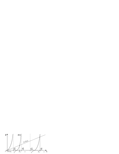
Figure 2. The limit eigenvalues $\lambda_{0}=\mu_{j}$

Remark 1.

If $Q_{0}$ is a ball of radius $0<a<1/2$, i.e $Q_{0}=B_{a}=\{y:|y|<a\}+y_{0}$, then we have an explicit representation for $\beta(\lambda)$. Indeed, for $\lambda_{0}\not\in\sigma_{D}$ the solution of (28) is radially symmetric and (placing the origin in the ball’s centre) reads

$$\eta(y)=|y|^{\frac{2-n}{2}}J_{\frac{n-2}{2}}(\lambda_{0}^{1/2}|y|)\left(|a|^{\frac{2-n}{2}}J_{\frac{n-2}{2}}(\lambda_{0}^{1/2}a)\right)^{-1},$$

where $J_{\frac{n-2}{2}}(|y|)$ is Bessel function. Further, we have

$$B(\lambda_{0})=\lambda_{0}\langle\eta\rangle=-\int_{\partial B_{a}}{\frac{\partial\eta}{\partial n_{y}}}dy=$$

$$=-\frac{1}{a}|\Gamma|\left(1-n/2+a\lambda_{0}^{1/2}J_{\frac{n-2}{2}}^{\prime}(\lambda_{0}^{1/2}a)/J_{\frac{n-2}{2}}(\lambda_{0}^{1/2}a)\right).$$

Using (37), (35) we obtain

$$\beta(\lambda)=\lambda(1-|B_{a}|)-\frac{1}{a}|\Gamma|\left(1-n/2+a\lambda^{1/2}J_{\frac{n-2}{2}}^{\prime}(\lambda^{1/2}a)/J_{\frac{n-2}{2}}(\lambda^{1/2}a)\right).$$

In particular, for $n=3$ we have,

$$B(\lambda_{0})=\lambda_{0}\langle\eta\rangle={4\pi a}\left(1-a\lambda_{0}^{1/2}\,\emph{cotan}\,(\lambda_{0}^{1/2}a)\right),$$

$$\beta(\lambda)=\lambda(1-4\pi a^{3}/3)+4\pi a\left(1-a\lambda^{1/2}\,\emph{cotan}\,(\lambda^{1/2}a)\right).$$

We next explore in detail the further steps in the method of asymptotic expansions, to determine $v^{0}$, etc. Let us consider a $K$-dimensional eigenspace ($K\geq 1$) for a given eigenvalue $\lambda_{0}$ of (29), and let $\zeta_{1},\dots,\zeta_{K}$ be associated linearly independent eigenfunctions. Then, (25) and (26) imply

(39) $$w_{0}(x,y)=\sum_{k=1}^{K}c_{k}(x)\zeta_{k}(y).$$

Following Theorem 3.1 we distinguish two cases:

• $\lambda_{0}\not\in\sigma_{D}$. In this case (28) and (25) suggest

  (40) $$w_{0}(x,y)=v^{0}(x)\eta(y),$$

  and (10) implies $v^{0}\not\equiv 0$.

• $\lambda_{0}\in\sigma_{D}$. The latter means $\lambda_{0}=\lambda^{D}_{j}$ for some $j$. This includes two further possibilities:

  • The eigenspace of (27) has an eigenfunction $\phi_{j}^{*}$ with a non-zero mean. Since the solvability conditions for (25) include

    (41) $$v^{0}(x)\langle\phi_{j}^{*}\rangle\,=\,0,$$

    necessarily $v^{0}\equiv 0$. Moreover, with $K_{D}$ denoting the multiplicity of $\lambda_{j}^{D}$ as of the eigenvalue of the Dirichlet problem (27), necessarily $K_{D}\geq 2$: if $K_{D}=1$ then $w_{0}=C(x)\phi_{j}^{*}$ and thus (26) implies $C(x)\equiv 0$ and $w_{0}\equiv 0$ contradicting to (10). Hence $w_{0}$ is given by (39) with $K=K_{D}-1$, with $\zeta_{k}$, $k=1,...,K$ being linearly independent eigenfunctions of (27) with zero mean (such $K$ eigenfunctions exist).

  • All of the eigenfunctions corresponding $\lambda^{D}_{j}$ have a zero mean. In this case $w_{0}$ is again given by (39), with $K=K_{D}$ if $\langle\eta\rangle\neq 0$ i.e. $B(\lambda_{0})\neq 0$ and $K=K_{D}+1$ if $B(\lambda_{0})=0$ with $\zeta_{K_{D}+1}=\eta$ where $\eta(y)$ is any solution of (28).

3.1. Case (a): $\lambda_{0}\not\in\sigma_{D}$

In this case $\lambda_{0}$ are solutions of (38). There is a countable set of $\lambda_{0}=\mu_{j}$, $j=1,2,\dots$ as Figure 2 illustrates. Note that this includes $\lambda_{0}=0$. Function $\beta$ blows up at the points $\lambda^{D}_{j}$, which are eigenvalues of (27) having an eigenfunction with a non-zero mean, monotonically increasing between such points. It also directly follows from (37) that $\beta(\lambda)>|Q_{1}|\lambda$ for $\lambda\in(0,\lambda^{D}_{1})$, implying $\lambda^{D}_{1}<\mu_{2}<\lambda^{D}_{2}$. Let $\lambda_{0}$ satisfying (38) be fixed.

We consider problem (23) taking into account (40), i.e.

(42) $$-\Delta_{y}v_{1}(x,y)=0\quad\mbox{in}\quad\Omega\times{{Q}}_{1},\qquad\frac{\partial v_{1}}{\partial n_{y}}\Big{|}_{y\in\Gamma}=-\frac{\partial v^{0}}{\partial n_{x}}\Big{|}_{y\in\Gamma}+v^{0}(x)\frac{\partial\eta}{\partial n_{y}}\Big{|}_{y\in\Gamma},$$

where $\eta(y)$ solves (28) and is given by (35). Hence $v_{1}$ is a solution to a problem depending linearly on $v^{0}$ and $\nabla_{x}v^{0}$, implying

(43) $$v_{1}(x,y)=v^{0}(x){\mathcal{N}}(y)+\frac{\partial v^{0}}{\partial x_{j}}N_{j}(y)+v_{1}^{*}(x),$$

with an arbitrary function $v_{1}^{*}(x)$. The choice of $v_{1}^{*}$ does not affect the subsequent constructions, so we set for simplicity $v_{1}^{*}\equiv 0$. In (43) functions $N_{j}$ and ${\mathcal{N}}$ are solutions to the problems

(44) $$\Delta_{y}N_{j}(y)=0\quad\mbox{in}\quad Q_{1},\qquad\frac{\partial N_{j}}{\partial n_{y}}\Big{|}_{y\in\Gamma}=-n_{j}(y),$$

and

(45) $$\Delta_{y}{\mathcal{N}}(y)=0\quad\mbox{in}\quad Q_{1},\qquad\frac{\partial{\mathcal{N}}}{\partial n_{y}}\Big{|}_{y\in\Gamma}=\frac{\partial\eta}{\partial n_{y}}\Big{|}_{y\in\Gamma}.$$

Solvability of (45) requires

$$\int_{\Gamma}\frac{\partial\eta}{\partial n_{y}}\,dy=0,$$

which is equivalent to (34) and is hence already assured. Since the solutions of (44) and (45) are unique up to an arbitrary constant, we fix those by choosing

$$\int_{Q_{1}}N_{j}(y)\,dy\,=\,\int_{Q_{1}}{\mathcal{N}}(y)\,dy=0.$$

We next consider the problem for $w_{1}$, which from (15) and (17) combined with (40) reads

(46) $$-\Delta_{y}w_{1}-\lambda_{0}w_{1} =\lambda_{1}v^{0}\eta+2\displaystyle\frac{\partial v^{0}}{\partial x_{j}}\frac{\partial\eta}{\partial y_{j}}\quad\mbox{in}\quad\Omega\times{{Q}}_{0},$$

(47) $$w_{1}\Big{|}_{y\in\Gamma} =\displaystyle v^{0}{\mathcal{N}}(y)\Big{|}_{y\in\Gamma}+\frac{\partial v^{0}}{\partial x_{j}}N_{j}(y)\Big{|}_{y\in\Gamma}.$$

Since the problem depends linearly on $v^{0}$, $\lambda_{1}v^{0}$ and $\frac{\partial v^{0}}{\partial x_{j}}$, the solution admits representation

(48) $$w_{1}(x,y)=\frac{\partial v^{0}}{\partial x_{j}}(x){\mathcal{M}}_{j}(y)+v^{0}(x){\mathcal{P}}(y)+\lambda_{1}v^{0}(x){\mathcal{R}}(y),$$

where functions ${\mathcal{M}}_{j}$, ${\mathcal{P}}$ and ${\mathcal{R}}$ are solutions to the problems

(49) $$-\Delta_{y}{\mathcal{M}}_{j}-\lambda_{0}{\mathcal{M}}_{j}=2\frac{\partial\eta}{\partial y_{j}}(y)\quad\mbox{in}\quad Q_{0},\qquad{\mathcal{M}}_{j}\Big{|}_{\Gamma}=N_{j}\Big{|}_{\Gamma},$$

(50) $$-\Delta_{y}{\mathcal{P}}-\lambda_{0}{\mathcal{P}}=0\quad\mbox{in}\quad Q_{0},\qquad{\mathcal{P}}\Big{|}_{\Gamma}={\mathcal{N}}\Big{|}_{\Gamma},$$

and

(51) $$-\Delta_{y}{\mathcal{R}}-\lambda_{0}{\mathcal{R}}=\eta(y)\quad\mbox{in}\quad Q_{0},\qquad{\mathcal{R}}\Big{|}_{\Gamma}=0.$$

Since by the assumption $\lambda_{0}\not\in\sigma_{D}$, all the problems (49) – (51) are uniquely solvable.

The problem for $v_{2}$ is in turn given by (13) and (20), whose solvability condition hence reads

(52) $$\int_{Q_{1}}\left(\Delta_{x}v_{0}+\lambda_{0}v_{0}+2\frac{\partial^{2}v_{1}}{\partial x_{j}\partial y_{j}}\right)\,dy=\int_{\Gamma}\left(-\frac{\partial v_{1}}{\partial n_{x}}+\frac{\partial w_{1}}{\partial n_{y}}+\frac{\partial w_{0}}{\partial n_{x}}\right)\,dy,$$

with functions $v_{1}$, $w_{1}$ and $w_{0}$ given by (43), (48) and (40) respectively.

Appendix A provides a detailed calculation showing that the above yields the following equations for $v^{0}$:

(53) $$-\,\mbox{div}\,A^{\mbox{\scriptsize hom}}\nabla_{x}v^{0} = \nu(\lambda_{1})v^{0}\quad\mbox{in}\quad\Omega,$$

(54) $$v^{0}\Big{|}_{\partial\Omega} = 0.$$

Here $A^{\mbox{\scriptsize hom}}=\left(A^{\mbox{\scriptsize hom}}_{jk}\right)_{j,k=1}^{n}$ is the classical homogenized matrix for periodic perforated domains, see e.g. [11]

(55) $$A^{\mbox{\scriptsize hom}}_{jk}=|Q_{1}|\delta_{jk}+\int_{Q_{1}}\frac{\partial N_{k}}{\partial y_{j}}\,dy;$$

(56) $$\nu(\lambda_{1})={\mathcal{C}}\lambda_{1}+\lambda_{0}\Big{(}|Q_{1}|+\int_{Q_{0}}{\mathcal{P}}\,dy\Big{)},$$

where

(57) $${\mathcal{C}}:=\int_{Q_{0}}\eta^{2}dy>0.$$

Note that the problem (53)–(54) involves $\nu=\nu(\lambda_{1})$ as a spectral parameter.

The spectrum of (53)–(54) consists of a countable set of eigenvalues

(58) $$0<\nu_{1}<\nu_{2}\leq\dots\leq\nu_{n}\leq\dots\to+\infty.$$

Corresponding eigenfunctions $v_{n}$ form an orthonormal basis in $L_{2}(\Omega)$,

$$\int_{\Omega}v^{0}_{n}v^{0}_{m}\,dx=\delta_{nm}.$$

Fixing an eigenvalue $\nu$ of (53), (54) with corresponding eigenfunction $v^{0}$ of unit norm in $L_{2}(\Omega)$, according to (56) we find

(59) $$\lambda_{1}={\mathcal{C}}^{-1}\left(\nu-\lambda_{0}\Big{(}|Q_{1}|+\int_{Q_{0}}{\mathcal{P}}\,dy\Big{)}\right).$$

The following diagram summarizes the algorithm for constructing the first terms of the asymptotic expansions (for the case $\lambda_{0}\not\in\sigma_{D}$)

$$\left.\begin{array}[]{lcrcl}N_{j}&\stackrel{{\scriptstyle\eqref{A hom}}}{{\rightarrow}}&A^{\mbox{\scriptsize hom}}&\stackrel{{\scriptstyle\eqref{homogenized problem eq}}}{{\rightarrow}}&\nu,v^{0}\\ \lambda_{0}&\stackrel{{\scriptstyle\eqref{probleta}}}{{\rightarrow}}&\eta&\stackrel{{\scriptstyle\eqref{problem cN}}}{{\rightarrow}}&{\mathcal{N}}\end{array}\right\}\left.\begin{array}[]{ll}\stackrel{{\scriptstyle\eqref{lm1}}}{{\rightarrow}}&\lambda_{1}\\ \stackrel{{\scriptstyle\eqref{representation v1}}}{{\rightarrow}}&v_{1}\\ \stackrel{{\scriptstyle\eqref{problem cM}-\eqref{problem cR}}}{{\rightarrow}}&{\mathcal{M}},{\mathcal{P}},{\mathcal{R}}\\ \stackrel{{\scriptstyle\eqref{case1w0}}}{{\rightarrow}}&w_{0}\end{array}\right\}\stackrel{{\scriptstyle\eqref{representation w1}}}{{\rightarrow}}w_{1}\stackrel{{\scriptstyle\eqref{eq v2},\eqref{bc v2}}}{{\rightarrow}}v_{2}.$$

We can additionally construct $w_{2}$ from (16) and (17), whose unique solution exists for any choice of $\lambda_{2}$. For purposes of the justification of the first two terms in the asymptotics (the next section) it is sufficient to set $\lambda_{2}=0$ and fix the corresponding solution $w_{2}$.

This completes constructing a formal asymptotic approximation, which we now summarize. We introduce an approximate eigenvalue

(60) $$\Lambda_{\varepsilon}=\lambda_{0}+\varepsilon\lambda_{1},$$

and corresponding approximate eigenfunction

(61) $$W_{\varepsilon}(x)=\left\{\begin{array}[]{ll}\displaystyle v^{0}(x)+\varepsilon v_{1}\left(x,\frac{x}{\varepsilon}\right)+\varepsilon^{2}v_{2}\left(x,\frac{x}{\varepsilon}\right),&x\in\Omega_{1}^{\varepsilon},\\ \displaystyle w_{0}\left(x,\frac{x}{\varepsilon}\right)+\varepsilon w_{1}\left(x,\frac{x}{\varepsilon}\right)+\varepsilon^{2}w_{2}\left(x,\frac{x}{\varepsilon}\right),&x\in\Omega_{0}^{\varepsilon}.\end{array}\right.$$

The essence of the above formal asymptotic construction is that the action of differential operator ${{\mathcal{A}^{\varepsilon}}}$ on $W_{\varepsilon}$ defined by

(62) $${{\mathcal{A}^{\varepsilon}}}W_{\varepsilon}\,:=\,\,\mbox{div}\,(a_{\varepsilon}\nabla W_{\varepsilon})+\Lambda_{\varepsilon}\rho_{\varepsilon}W_{\varepsilon}$$

produces a small right-hand side in both $\Omega_{1}^{\varepsilon}$ and $\Omega_{0}^{\varepsilon}$, and on the interface $\Gamma^{\varepsilon}$ in the following sense.

Lemma 3.2.

$(i)\,\,\,\displaystyle\max_{\bar{\Omega}^{\varepsilon}_{1}}\left|\emph{\, \mbox{div}\,}(a_{\varepsilon}\nabla W_{\varepsilon})+\Lambda_{\varepsilon}\rho_{\varepsilon}W_{\varepsilon}\right|\leq C\varepsilon.$

$(ii)\,\,\,\displaystyle\max_{\bar{\Omega}^{\varepsilon}_{0}}\left|\emph{\, \mbox{div}\,}(a_{\varepsilon}\nabla W_{\varepsilon})+\Lambda_{\varepsilon}\rho_{\varepsilon}W_{\varepsilon}\right|\leq C\varepsilon^{2}.$

$(iii)\,\,\,\displaystyle\max_{{\Gamma}^{\varepsilon}}\left|\left.a_{\varepsilon}\frac{\partial W_{\varepsilon}}{\partial n}\right|_{0}-\left.a_{\varepsilon}\frac{\partial W_{\varepsilon}}{\partial n}\right|_{1}\right|\leq C\varepsilon^{2}.$

Proof.

$(i)\,$ Since the function $W_{\varepsilon}$ is two-scale by the construction, in $\Omega^{\varepsilon}_{1}$

$$\,\mbox{div}\,( a_{\varepsilon}\nabla W_{\varepsilon})+\Lambda_{\varepsilon}\rho_{\varepsilon}W_{\varepsilon}=$$

$$=\left(\varepsilon^{-2}\Delta_{y}+\varepsilon^{-1}2\frac{\partial^{2}}{\partial x_{j}\partial y_{j}}+\Delta_{x}+\lambda_{0}+\varepsilon\lambda_{1}\right)(v^{0}(x)+\varepsilon v_{1}(x,y)+\varepsilon^{2}v_{2}(x,y))|_{y=\frac{x}{\varepsilon}}=$$

$$=\left\{\varepsilon^{-1}\Delta_{y}v_{1}(x,y)+\varepsilon^{0}\left(\Delta_{y}v_{2}+2\frac{\partial^{2}v_{1}}{\partial x_{j}\partial y_{j}}+\Delta_{x}v^{0}+\lambda_{0}v^{0}\right)+\right.$$

(63) $$+\left.\left.\varepsilon^{1}\left(2\frac{\partial^{2}v_{2}}{\partial x_{j}\partial y_{j}}+\Delta_{x}v_{1}+\lambda_{1}v^{0}+\lambda_{0}v_{1}\right)+\varepsilon^{2}(\Delta_{x}v_{2}+\lambda_{1}v_{1}+\lambda_{0}v_{2})+\varepsilon^{3}\lambda_{1}v_{2}\right\}\right|_{y=\frac{x}{\varepsilon}}.$$

Since $v_{1}$ is a solution to (42), the coefficient of $\varepsilon^{-1}$ vanishes. The same is with the coefficient of $\varepsilon^{0}$ since $v_{2}$ satisfies (13). Functions $v^{0}$, $v_{1}$ and $v_{2}$ are solutions of elliptic problems with smooth enough coefficients to guarantee belonging solutions to $C^{2}$. Thus, maxima for coefficients of $\varepsilon^{1}$, $\varepsilon^{2}$ and $\varepsilon^{3}$ in (63) exist.

$(ii)\,$ Similarly, in $\Omega^{\varepsilon}_{0}$

$$\,\mbox{div}\,(a_{\varepsilon}\nabla W_{\varepsilon})+\Lambda_{\varepsilon}\rho_{\varepsilon}W_{\varepsilon}=$$

$$=\left(\varepsilon^{-1}\Delta_{y}+2\frac{\partial^{2}}{\partial x_{j}\partial y_{j}}+\varepsilon\Delta_{x}+\varepsilon^{-1}\lambda_{0}+\lambda_{1}\right)(w_{0}(x,y)+\varepsilon w_{1}(x,y)+\varepsilon^{2}w_{2}(x,y))|_{y=\frac{x}{\varepsilon}}=$$

$$=\left\{\varepsilon^{-1}(\Delta_{y}w_{0}+\lambda_{0}w_{0})+\varepsilon^{0}\left(\Delta_{y}w_{1}+2\frac{\partial^{2}w_{0}}{\partial x_{j}\partial y_{j}}+\lambda_{0}w_{1}+\lambda_{1}w_{0}\right)+\right.$$

$$+\varepsilon^{1}\left(\Delta_{y}w_{2}+2\frac{\partial^{2}w_{1}}{\partial x_{j}\partial y_{j}}+\Delta_{x}w_{0}+\lambda_{0}w_{2}+\lambda_{1}w_{1}\right)+$$

$$+\left.\left.\varepsilon^{2}\left(2\frac{\partial^{2}w_{2}}{\partial x_{j}\partial y_{j}}+\Delta_{x}w_{1}+\lambda_{1}w_{2}\right)+\varepsilon^{3}\Delta_{x}w_{2}\right\}\right|_{y=\frac{x}{\varepsilon}}.$$

Since $w_{0}(x,y)=v^{0}(x)\eta(y)$ is chosen according to (28), the coefficient of $\varepsilon^{-1}$ vanishes. The coefficient of $\varepsilon^{0}$ vanishes due to (46). Further, $w_{2}$ satisfies (16) with $\lambda_{2}=0$ and thus the coefficient of $\varepsilon^{1}$ is zero as well. Since $w_{1}$ and $w_{2}$ are solutions of elliptic problems with smooth enough coefficients, the maxima of the coefficients of $\varepsilon^{2}$ and $\varepsilon^{3}$ exist.

$(iii)\,$ Using (21), we obtain

$$\left.a_{\varepsilon}\frac{\partial W_{\varepsilon}}{\partial n}\right|_{0} -\left.a_{\varepsilon}\frac{\partial W_{\varepsilon}}{\partial n}\right|_{1}=\left(\frac{\partial}{\partial n_{y}}+\varepsilon\frac{\partial}{\partial n_{x}}\right)(w_{0}(x,y)+\varepsilon w_{1}(x,y)+\varepsilon^{2}w_{2}(x,y))\Big{|}_{\begin{subarray}{c}x\in{\Gamma}^{\varepsilon}\\ y\in{\Gamma}\hskip 4.2679pt\end{subarray}}-$$

$$-\left(\varepsilon^{-1}\frac{\partial}{\partial n_{y}}+\frac{\partial}{\partial n_{x}}\right)(v^{0}(x)+\varepsilon v_{1}(x,y)+\varepsilon^{2}v_{2}(x,y))\Big{|}_{\begin{subarray}{c}x\in{\Gamma}^{\varepsilon}\\ y\in{\Gamma}\hskip 4.2679pt\end{subarray}}=$$

$$=\varepsilon^{0}\left(\frac{\partial w_{0}}{\partial n_{y}}-\frac{\partial v_{1}}{\partial n_{y}}-\frac{\partial v^{0}}{\partial n_{x}}\right)\Big{|}_{\begin{subarray}{c}x\in{\Gamma}^{\varepsilon}\\ y\in{\Gamma}\hskip 4.2679pt\end{subarray}}+\varepsilon^{1}\left(\frac{\partial w_{1}}{\partial n_{y}}+\frac{\partial w_{0}}{\partial n_{x}}-\frac{\partial v_{2}}{\partial n_{y}}-\frac{\partial v_{1}}{\partial n_{x}}\right)\Big{|}_{\begin{subarray}{c}x\in{\Gamma}^{\varepsilon}\\ y\in{\Gamma}\hskip 4.2679pt\end{subarray}}+$$

(64) $$+\varepsilon^{2}\left(\frac{\partial w_{2}}{\partial n_{y}}+\frac{\partial w_{1}}{\partial n_{x}}-\frac{\partial v_{2}}{\partial n_{x}}\right)\Big{|}_{\begin{subarray}{c}x\in{\Gamma}^{\varepsilon}\\ y\in{\Gamma}\hskip 4.2679pt\end{subarray}}+\varepsilon^{3}\frac{\partial w_{2}}{\partial n_{x}}\Big{|}_{\begin{subarray}{c}x\in{\Gamma}^{\varepsilon}\\ y\in{\Gamma}\hskip 4.2679pt\end{subarray}}.$$

The coefficients of $\varepsilon^{0}$ and $\varepsilon^{1}$ vanish because of (23) and (20) respectively. The rest of the coefficients are smooth enough to guarantee that their maxima for $x\in{\Gamma}^{\varepsilon}$ and $y\in\Gamma$ exist. ∎

3.2. Case (b): $\lambda_{0}=\lambda_{j}^{D}$

For simplicity, we consider here only the case of eigenvalues of multiplicity $K=1$ with zero mean eigenfunction ($\phi=\phi_{j}$), assuming additionally $\lambda_{0}$ is not a solution of (36). All other degenerate cases, see page 41, could be considered similarly.

In this case we can introduce a refined approximation for the eigenfunction

(65) $$W_{\varepsilon}^{*}(x)=\left\{\begin{array}[]{ll}\displaystyle\varepsilon v_{1}\left(x,\frac{x}{\varepsilon}\right)+\varepsilon^{2}v_{2}\left(x,\frac{x}{\varepsilon}\right),&x\in\Omega_{1}^{\varepsilon},\\ \displaystyle w_{0}\left(x,\frac{x}{\varepsilon}\right)+\varepsilon w_{1}\left(x,\frac{x}{\varepsilon}\right)+\varepsilon^{2}w_{2}\left(x,\frac{x}{\varepsilon}\right),&x\in\Omega_{0}^{\varepsilon}.\end{array}\right.$$

where

(66) $$w_{0}(x,y)=c(x)\phi(y).$$

Lemma 3.3.

Let $c\in C^{3}(\Omega)$, then there exist smooth functions $v_{1},w_{1},v_{2},w_{2}$ and a constant $\lambda_{1}$ such that $\Lambda_{\varepsilon}=\lambda_{j}^{D}+\varepsilon\lambda_{1}$ and $W_{\varepsilon}^{*}$ defined by (65) satisfy

• $W_{\varepsilon}^{*}(x)\in C(\Omega),$

• $\displaystyle\max_{\bar{\Omega}^{\varepsilon}_{1}}\left|\emph{\, \mbox{div}\,}(a_{\varepsilon}\nabla W_{\varepsilon}^{*})+\Lambda_{\varepsilon}\rho_{\varepsilon}W_{\varepsilon}^{*}\right|\leq C\varepsilon,$

• $\displaystyle\max_{\bar{\Omega}^{\varepsilon}_{0}}\left|\emph{\, \mbox{div}\,}(a_{\varepsilon}\nabla W_{\varepsilon}^{*})+\Lambda_{\varepsilon}\rho_{\varepsilon}W_{\varepsilon}^{*}\right|\leq C\varepsilon^{2},$

• $\displaystyle\max_{{\Gamma}^{\varepsilon}}\left|\left.a_{\varepsilon}\frac{\partial W_{\varepsilon}^{*}}{\partial n}\right|_{0}-\left.a_{\varepsilon}\frac{\partial W_{\varepsilon}^{*}}{\partial n}\right|_{1}\right|\leq C\varepsilon^{2}.$

Proof.

See Appendix B. ∎

4. Justification of asymptotics

4.1. Operator formulation

We use a standard notation for Lebesgue and Sobolev spaces: $L^{2}_{p}(\Omega)$ is a $p$-weighted $L^{2}$-space of square-integrable functions in $\Omega$. Notation $(\cdot,\cdot)_{H}$ is used for a scalar product in a Hilbert space $H$.

Let ${\mathcal{L}^{\varepsilon}}=L^{2}_{\rho_{\varepsilon}}(\Omega)$ and ${\mathcal{H}^{\varepsilon}}$ be $H^{1}_{0}(\Omega)$ Sobolev space with a scalar product

$$(u,v)_{\mathcal{H}^{\varepsilon}}=\int_{\Omega}a_{\varepsilon}(x)\nabla u\cdot\nabla v\,dx+\int_{\Omega}\rho_{\varepsilon}(x)uv\,dx.$$

Following a standard procedure, see e.g. [11], we introduce a bounded operator ${\mathcal{B}_{\varepsilon}}:{\mathcal{L}^{\varepsilon}}\to{\mathcal{L}^{\varepsilon}}$ such that

(67) $$({\mathcal{B}_{\varepsilon}}f,v)_{\mathcal{H}^{\varepsilon}}=(f,v)_{\mathcal{L}^{\varepsilon}},\quad\forall v\in{\mathcal{H}^{\varepsilon}}.$$

In other words ${\mathcal{B}_{\varepsilon}}f=u_{\varepsilon}$, where $u_{\varepsilon}$ is the solution of the problem

(68) $$-\,\mbox{div}\,(a_{\varepsilon}\nabla u_{\varepsilon})+\rho_{\varepsilon}u_{\varepsilon} = \rho_{\varepsilon}f,\quad x\in\Omega,$$

(69) $$u_{\varepsilon}|_{\partial\Omega} = 0,$$

(70) $$u_{\varepsilon}\Big{|}_{1}=u_{\varepsilon}\Big{|}_{0},\quad\frac{\partial u_{\varepsilon}}{\partial n_{x}}\Big{|}_{1}=\varepsilon\frac{\partial u_{\varepsilon}}{\partial n_{x}}\Big{|}_{0}.$$

Note that operator ${\mathcal{B}_{\varepsilon}}$ is positive, self-adjoint and compact for any fixed $\varepsilon>0$ (since its image is in ${\mathcal{H}^{\varepsilon}}$). Eigenvalue problem (2) is equivalent to

(71) $${\mathcal{B}_{\varepsilon}}u_{\varepsilon}=(\lambda^{\varepsilon}+1)^{-1}u_{\varepsilon}\quad\text{in}\quad{\mathcal{L}^{\varepsilon}}.$$

Hence the spectrum of the problem consists of a countable set of eigenvalues

$$0<\lambda^{\varepsilon}_{1}<\lambda^{\varepsilon}_{2}\leq\dots\leq\lambda^{\varepsilon}_{k}\leq\dots\to+\infty,$$

with the only accumulation point at $+\infty$. Moreover, the set of corresponding eigenfunctions is complete in ${\mathcal{L}^{\varepsilon}}$.

4.2. Case (a)

In this Section we justify the leading terms of asymptotic expansions constructed above in case $\lambda_{0}\not\in\sigma_{D}$ and thus $v^{0}\not\equiv 0$, see Section 3.1. Let $\lambda_{0}$ be a solution to equation (38). All the functions ($\eta$, $N_{j}$, ${\mathcal{N}}$, ${\mathcal{M}}$, ${\mathcal{P}}$, ${\mathcal{R}}$, $w_{0}$, $w_{1}$, $v_{1}$ and $w_{2}$, $v_{2}$) are as defined in Section 3.1. We also fix $\lambda_{1}$ according to (59). The approximate eigenvalue $\Lambda_{\varepsilon}$ and eigenfunction $W_{\varepsilon}$ are given by (60) and (61) respectively.

Notice that although $W_{\varepsilon}\in H^{1}(\Omega)$ since $W_{\varepsilon}\Big{|}_{1}=W_{\varepsilon}\Big{|}_{0}$, it does not satisfy the zero Dirichlet boundary conditions on $\partial\Omega$. To fix this we introduce the following boundary-layer corrector to our approximation.

Lemma 4.1.

There exists a corrector $V_{\varepsilon}$ solving the problem

(72) $$-\emph{div}(a_{\varepsilon}\nabla V_{\varepsilon}) +\rho_{\varepsilon}V_{\varepsilon}=0\quad\text{in}\quad\Omega,$$

(73) $$V_{\varepsilon}|_{\partial\Omega}=-W_{\varepsilon}|_{\partial\Omega},\quad V_{\varepsilon}\Big{|}_{1} =V_{\varepsilon}\Big{|}_{0},\quad\frac{\partial V_{\varepsilon}}{\partial n}\Big{|}_{1}=\varepsilon\frac{\partial V_{\varepsilon}}{\partial n}\Big{|}_{0},$$

such that $U_{\varepsilon}=W_{\varepsilon}+V_{\varepsilon}\in H^{1}_{0}(\Omega)$  and  $\displaystyle\max_{\bar{\Omega}}|V_{\varepsilon}|\leq C\varepsilon.$

Proof.

Clearly such solution of (72), (73) does exist. On each of the subsets $\Omega^{\varepsilon}_{1}$ and $\Omega^{\varepsilon}_{0}$ the coefficients of (72) are smooth. Then the function $V_{\varepsilon}$ can reach its positive maximum or negative minimum only at the boundaries ${\Gamma}^{\varepsilon}$ or $\partial\Omega$. Let us prove that this cannot be ${\Gamma}^{\varepsilon}$. Suppose to the contrary the existence of $x_{*}\in{\Gamma}^{\varepsilon}$ such that $\displaystyle\max_{\bar{\Omega}}|V_{\varepsilon}|=|V_{\varepsilon}(x_{*})|$. The strong maximum principle yields that there is no more point inside $\Omega^{\varepsilon}_{1}$ or $\Omega^{\varepsilon}_{0}$ where the maximum is reached. Without loss of generality we assume $V_{\varepsilon}(x_{*})>V_{\varepsilon}(x)$ for any $x\in\Omega\backslash{\Gamma}^{\varepsilon}$ and $V_{\varepsilon}(x_{*})\geq 0$ (otherwise the point would be a positive maximum for $-V_{\varepsilon}$ and we would then consider $-V_{\varepsilon}$). Then by the virtue of Hopf’s Lemma [8, p.330] applied in the relevant component of $\Omega^{\varepsilon}_{0}$ we have

$$\left.\frac{\partial V_{\varepsilon}}{\partial n}\right|_{0}(x_{*})>0.$$

From transmission conditions (73) we have that the normal derivative on the $\Omega^{\varepsilon}_{1}$ side of domain is also positive. Therefore the value of $V_{\varepsilon}$ increases from the point $x_{*}$ inside $\Omega^{\varepsilon}_{1}$ in the $n$-direction and hence $x_{*}$ is not a point of maximum of $V_{\varepsilon}$ in $\Omega^{\varepsilon}_{1}$. The contradiction proves that $|V_{\varepsilon}|$ reaches it’s maximum at $\partial\Omega$. Then, from boundary conditions (73),

$$\max_{\bar{\Omega}}|V_{\varepsilon}|=\max_{\partial\Omega}|V_{\varepsilon}|=\max_{\partial\Omega}|W_{\varepsilon}|\leq\\ \varepsilon\max_{\partial\Omega}\left|v_{1}\left(x,\frac{x}{\varepsilon}\right)+\varepsilon v_{2}\left(x,\frac{x}{\varepsilon}\right)\right|+$$

$$\varepsilon\max_{\partial\Omega}\left|w_{1}\left(x,\frac{x}{\varepsilon}\right)+\varepsilon w_{2}\left(x,\frac{x}{\varepsilon}\right)\right|\leq C\varepsilon.$$

Obviously $U_{\varepsilon}=W_{\varepsilon}+V_{\varepsilon}$ satisfies zero boundary condition on $\partial\Omega$ and thus belongs to $H^{1}_{0}(\Omega)$. ∎

Lemma 4.2.

The constructed corrector $V_{\varepsilon}$ satisfies the estimate $\|V_{\varepsilon}\|_{\mathcal{L}^{\varepsilon}}\leq C\varepsilon^{3/4}$.

Proof.

Let $\chi\in C^{\infty}(\mathbb{R})$ and $\chi(t)=0,\ t<1$ and $\chi(t)=1,\ t>2$. Let us define a family of cut-off functions:

$$\chi_{\varepsilon}(x)=\chi\left(\varepsilon^{-1/2}\,\mbox{dist}\,(x,\partial\Omega)\right),\quad x\in\Omega.$$

Then $\chi_{\varepsilon}:\Omega\to\mathbb{R}$ satisfies the properties

• $\chi_{\varepsilon}(x)=0$ if $\,\mbox{dist}\,(x,\partial\Omega)\leq\varepsilon^{1/2}$,

• $\chi_{\varepsilon}(x)=1$ if $\,\mbox{dist}\,(x,\partial\Omega)\geq 2\varepsilon^{1/2}$,

• $|\nabla\chi_{\varepsilon}|\leq C\varepsilon^{-1/2}$ and $|\text{supp}\,{\nabla\chi_{\varepsilon}}|\leq C\varepsilon^{1/2}$,

where “supp” denotes a function support, and $|\text{supp}\,{\cdot}|$ is the measure of the corresponding support. Multiplying (72) by $\chi_{\varepsilon}^{2}V_{\varepsilon}$ and integrating by parts, we obtain

(74) $$\int_{\Omega}a_{\varepsilon}\nabla V_{\varepsilon}\cdot\nabla(\chi_{\varepsilon}^{2}V_{\varepsilon})\,dx+\int_{\Omega}\rho_{\varepsilon}\chi_{\varepsilon}^{2}V_{\varepsilon}^{2}\,dx=0.$$

Then using the identity

$$\nabla V_{\varepsilon}\cdot\nabla(\chi_{\varepsilon}^{2}V_{\varepsilon})=|\nabla(\chi_{\varepsilon}V_{\varepsilon})|^{2}-V_{\varepsilon}^{2}|\nabla\chi_{\varepsilon}|^{2},$$

we get from (74)

(75) $$\int_{\Omega}a_{\varepsilon}|\nabla(\chi_{\varepsilon}V_{\varepsilon})|^{2}\,dx+\int_{\Omega}\rho_{\varepsilon}\chi_{\varepsilon}^{2}V_{\varepsilon}^{2}\,dx=\int_{\Omega}a_{\varepsilon}V_{\varepsilon}^{2}|\nabla\chi_{\varepsilon}|^{2}\,dx,$$

implying

(76) $$\int_{\Omega}\rho_{\varepsilon}\chi_{\varepsilon}^{2}V_{\varepsilon}^{2}\,dx\leq\int_{\Omega}a_{\varepsilon}V_{\varepsilon}^{2}|\nabla\chi_{\varepsilon}|^{2}\,dx.$$

Lemma 4.1 provides the estimate $V_{\varepsilon}^{2}\leq C\varepsilon^{2}$. Moreover, $|\text{supp}\,{\nabla\chi_{\varepsilon}}|\leq C\varepsilon^{1/2}$ and $|\nabla\chi_{\varepsilon}|^{2}\leq C\varepsilon^{-1}$. Therefore estimate (76) yields

(77) $$\|\chi_{\varepsilon}V_{\varepsilon}\|_{\mathcal{L}^{\varepsilon}}^{2}=\int_{\Omega}\rho_{\varepsilon}\chi_{\varepsilon}^{2}V_{\varepsilon}^{2}\,dx\leq C\varepsilon^{3/2}.$$

Similarly we estimate

(78) $$\|(1-\chi_{\varepsilon})V_{\varepsilon}\|_{\mathcal{L}^{\varepsilon}}^{2}=\int_{\Omega}\rho_{\varepsilon}(1-\chi_{\varepsilon})^{2}V_{\varepsilon}^{2}\,dx\leq C\varepsilon^{3/2},$$

since $|\text{supp}\,{(1-\chi_{\varepsilon})}|\leq C\varepsilon^{1/2}$ and $|\rho_{\varepsilon}|\leq C\varepsilon^{-1}$. Combining (77) and (78), we obtain $\|V_{\varepsilon}\|_{\mathcal{L}^{\varepsilon}}=\|(1-\chi_{\varepsilon})V_{\varepsilon}+\chi_{\varepsilon}V_{\varepsilon}\|_{\mathcal{L}^{\varepsilon}}\leq C\varepsilon^{3/4}.$ ∎

Lemma 4.3.

If $\varphi\in H^{1}_{0}(\Omega)$ then

(79) $$\Big{(}\int_{{\Gamma}^{\varepsilon}}|\varphi|^{2}\,dx\Big{)}^{1/2}\leq C\|\varphi\|_{\mathcal{H}^{\varepsilon}}.$$

Proof.

Extend function $\varphi$ by zero to whole of $\mathbb{R}^{n}$. Then (79) follows upon rescaling $y=x/\varepsilon$ from the standard trace estimates applied to each connected component of $\widetilde{Q}_{0}$ (which are shifts of $Q_{0}$). ∎

Lemma 4.4.

The corrected approximation $U_{\varepsilon}$ satisfies the estimate

$$\|{\mathcal{B}_{\varepsilon}}U_{\varepsilon}-(\Lambda_{\varepsilon}+1)^{-1}U_{\varepsilon}\|_{\mathcal{L}^{\varepsilon}}\leq\|{\mathcal{B}_{\varepsilon}}U_{\varepsilon}-(\Lambda_{\varepsilon}+1)^{-1}U_{\varepsilon}\|_{\mathcal{H}^{\varepsilon}}\leq C\varepsilon^{3/4}.$$

Proof.

For an arbitrary $\varphi\in{\mathcal{H}^{\varepsilon}}$ consider

$$|({\mathcal{B}_{\varepsilon}}U_{\varepsilon} -(\Lambda_{\varepsilon}+1)^{-1}U_{\varepsilon},\varphi)_{\mathcal{H}^{\varepsilon}}|=|\Lambda_{\varepsilon}+1|^{-1}|(U_{\varepsilon}-(\Lambda_{\varepsilon}+1){\mathcal{B}_{\varepsilon}}U_{\varepsilon},\varphi)_{\mathcal{H}^{\varepsilon}}|\leq$$

$$\leq C|(U_{\varepsilon},\varphi)_{\mathcal{H}^{\varepsilon}}-(\Lambda_{\varepsilon}+1)({\mathcal{B}_{\varepsilon}}U_{\varepsilon},\varphi)_{\mathcal{H}^{\varepsilon}}|=C|(U_{\varepsilon},\varphi)_{\mathcal{H}^{\varepsilon}}-(\Lambda_{\varepsilon}+1)(U_{\varepsilon},\varphi)_{\mathcal{L}^{\varepsilon}}|=$$

$$=C\left|\int_{\Omega}a_{\varepsilon}\nabla U_{\varepsilon}\nabla\varphi\,dx-\Lambda_{\varepsilon}\int_{\Omega}\rho_{\varepsilon}U_{\varepsilon}\varphi\,dx\right|\leq$$

(80) $$\leq C\left|\ \int_{\Omega_{0}^{\varepsilon}\cup\Omega_{1}^{\varepsilon}}\left(\,\mbox{div}\,(a_{\varepsilon}\nabla U_{\varepsilon})+\Lambda_{\varepsilon}\rho_{\varepsilon}U_{\varepsilon}\right)\varphi\,dx\right|+C\int_{{\Gamma}^{\varepsilon}}\left|\left.a_{\varepsilon}\frac{\partial U_{\varepsilon}}{\partial n}\right|_{0}-\left.a_{\varepsilon}\frac{\partial U_{\varepsilon}}{\partial n}\right|_{1}\right||\varphi|\,dx.$$

Denote the right-hand side of (80) by $F_{\varepsilon}(U_{\varepsilon},\varphi)$. Substituting $U_{\varepsilon}=W_{\varepsilon}+V_{\varepsilon}$ and taking into account (72) and (73),

$$F_{\varepsilon}(U_{\varepsilon},\varphi)\leq F_{\varepsilon}(W_{\varepsilon},\varphi)+C\left|(\Lambda_{\varepsilon}+1)\int_{\Omega}\rho_{\varepsilon}V_{\varepsilon}\varphi\,dx\right|\leq F_{\varepsilon}(W_{\varepsilon},\varphi)+C\|V_{\varepsilon}\|_{\mathcal{L}^{\varepsilon}}\|\varphi\|_{\mathcal{L}^{\varepsilon}}.$$

By Lemma 4.2 and obvious inequality $\|\varphi\|_{\mathcal{L}^{\varepsilon}}\leq\|\varphi\|_{\mathcal{H}^{\varepsilon}}$,

(81) $$F_{\varepsilon}(U_{\varepsilon},\varphi)\leq F_{\varepsilon}(W_{\varepsilon},\varphi)+C\varepsilon^{3/4}\|\varphi\|_{\mathcal{H}^{\varepsilon}}.$$

According to Lemma 3.2 $(i)$ and $(ii)$,

$$F_{\varepsilon}(W_{\varepsilon},\varphi)\leq C\varepsilon\|\varphi\|_{L^{2}(\Omega)}+C\int_{{\Gamma}^{\varepsilon}}\left|\left.a_{\varepsilon}\frac{\partial W_{\varepsilon}}{\partial n}\right|_{0}-\left.a_{\varepsilon}\frac{\partial W_{\varepsilon}}{\partial n}\right|_{1}\right||\varphi|\,dx.$$

Due to Lemmas 3.2 $(iii)$ and 4.3 the latter yields

(82) $$F_{\varepsilon}(W_{\varepsilon},\varphi)\leq C\varepsilon\|\varphi\|_{\mathcal{L}^{\varepsilon}}+C\varepsilon^{3/2}\Big{(}\int_{{\Gamma}^{\varepsilon}}|\varphi|^{2}\,dx\Big{)}^{1/2}\leq C\varepsilon\|\varphi\|_{\mathcal{H}^{\varepsilon}}.$$

Using (82), (81) in (80) yields

$$|({\mathcal{B}_{\varepsilon}}U_{\varepsilon}-(\Lambda_{\varepsilon}+1)^{-1}U_{\varepsilon},\varphi)_{\mathcal{H}^{\varepsilon}}|\leq C\varepsilon^{3/4}\|\varphi\|_{\mathcal{H}^{\varepsilon}}$$

for all $\varphi\in{\mathcal{H}^{\varepsilon}}$. Hence, $\|{\mathcal{B}_{\varepsilon}}U_{\varepsilon}-(\Lambda_{\varepsilon}+1)^{-1}U_{\varepsilon}\|_{\mathcal{H}^{\varepsilon}}\leq C\varepsilon^{3/4}$. ∎

Lemma 4.5.

$\|U_{\varepsilon}\|_{\mathcal{L}^{\varepsilon}}\geq C\varepsilon^{-1/2}.$

Proof.

By the triangle inequality we have

(83) $$\|U_{\varepsilon}\|_{\mathcal{H}^{\varepsilon}}\geq\|U_{\varepsilon}\|_{\mathcal{L}^{\varepsilon}}\geq\|W_{\varepsilon}\|_{\mathcal{L}^{\varepsilon}}-\|V_{\varepsilon}\|_{\mathcal{L}^{\varepsilon}}.$$

We consider

$$\|W_{\varepsilon}\|_{\mathcal{L}^{\varepsilon}}^{2} =\varepsilon^{-1}\int_{\Omega^{\varepsilon}_{0}}\left|w_{0}\left(x,\frac{x}{\varepsilon}\right)+\varepsilon w_{1}\left(x,\frac{x}{\varepsilon}\right)+\varepsilon^{2}w_{2}\left(x,\frac{x}{\varepsilon}\right)\right|^{2}\,dx+$$

$$+\int_{\Omega^{\varepsilon}_{0}}\left|v^{0}(x)+\varepsilon v_{1}\left(x,\frac{x}{\varepsilon}\right)+\varepsilon^{2}v_{2}\left(x,\frac{x}{\varepsilon}\right)\right|^{2}\,dx=$$

(84) $$=\varepsilon^{-1}\int_{\Omega^{\varepsilon}_{0}}\left|w_{0}\left(x,\frac{x}{\varepsilon}\right)\right|^{2}\,dx+O(1)=\varepsilon^{-1}\int_{\Omega^{\varepsilon}_{0}}\left|v^{0}(x)\eta\left(\frac{x}{\varepsilon}\right)\right|^{2}\,dx+O(1),\quad\varepsilon\to 0.$$

Extending $\eta:Q_{0}\to\mathbb{R}$ by zero onto entire periodicity cell $Q$, by the mean value property we obtain

(85) $$\int_{\Omega^{\varepsilon}_{0}}\left|v^{0}(x)\eta\left(\frac{x}{\varepsilon}\right)\right|^{2}\,dx\quad\rightarrow\quad C_{*}:=\langle\eta^{2}\rangle\int_{\Omega}\left|v^{0}(x)\right|^{2}\,dx\quad\text{as}\quad\varepsilon\to 0,$$

where $\langle\eta^{2}\rangle$ is the mean value of function $\eta^{2}$ over $Q$, namely

$$\langle\eta^{2}\rangle=\int_{Q}\eta^{2}(y)\,dy=\int_{Q_{0}}\eta^{2}(y)\,dy\,>0.$$

Since also $v^{0}(x)\not\equiv 0$, $C_{*}$ is positive. Therefore (85) and (84) yield

(86) $$\|W_{\varepsilon}\|_{\mathcal{L}^{\varepsilon}}=C_{*}^{1/2}\varepsilon^{-1/2}+o(\varepsilon^{-1/2}),\quad\varepsilon\to 0.$$

Due to Lemma 4.2 and (86), it follows from (83) that $\|U_{\varepsilon}\|_{\mathcal{L}^{\varepsilon}}\geq C_{*}^{1/2}\varepsilon^{-1/2}+o(\varepsilon^{-1/2})$ as $\varepsilon\to 0$. ∎

Theorem 4.6.

Let $\lambda_{0}$ be a solution to (38) such that $\lambda_{0}\neq\lambda^{D}_{j}$ and $\lambda_{1}$ is defined according to (59). Then

1. For sufficiently small $\varepsilon>0$ there exists an eigenvalue $\lambda^{\varepsilon}$ of (2) such that

(87) $$|\lambda^{\varepsilon}-\lambda_{0}-\varepsilon\lambda_{1}|\leq C_{1}\varepsilon^{5/4},$$

with constant $C_{1}$ independent of $\varepsilon$.

2. Let $W_{\varepsilon}$ be defined by (61) and $\widetilde{W_{\varepsilon}}=\|W_{\varepsilon}\|_{\mathcal{L}^{\varepsilon}}^{-1}W_{\varepsilon}$. Then there exist constants $c_{j}(\varepsilon)$ such that

(88) $$\Big{\|}\widetilde{W_{\varepsilon}}-\sum_{j\in J_{\varepsilon}}c_{j}(\varepsilon)u_{j}^{\varepsilon}\Big{\|}_{{\mathcal{L}^{\varepsilon}}}<C_{2}\varepsilon^{5/4},$$

where $J_{\varepsilon}=\{j:|\lambda_{j}^{\varepsilon}-\lambda_{0}-\varepsilon\lambda_{1}|<C\varepsilon^{5/4}\}$, and $\lambda_{j}^{\varepsilon}$, $u^{\varepsilon}_{j}$ are eigenvalues and (${\mathcal{L}^{\varepsilon}}$-normalized) eigenfunctions of (2), and the constants $C$ and $C_{2}$ are independent of $\varepsilon$.

Proof.

Application of classical lemma on “approximate eigenvalues”, e.g. [18], with $\widetilde{U}_{\varepsilon}=\|U_{\varepsilon}\|_{\mathcal{L}^{\varepsilon}}^{-1}U_{\varepsilon}$ as a test function and $\Lambda_{\varepsilon}=\lambda_{0}+\varepsilon\lambda_{1}$ as an approximate eigenvalue, ensures, via Lemmas 4.4 & 4.5, the existence of an eigenvalue $\mu_{\varepsilon}$ of operator ${\mathcal{B}_{\varepsilon}}$ such that

(89) $$|(\Lambda_{\varepsilon}+1)^{-1}-\mu_{\varepsilon}|\leq C\varepsilon^{5/4},$$

and delivers the estimate analogous to (88) with $u_{j}^{\varepsilon}$ being eigenfunctions of ${\mathcal{B}_{\varepsilon}}$ and $\widetilde{W_{\varepsilon}}$ replaced by $\widetilde{U}_{\varepsilon}$. It suffices to notice that the eigenfunctions of the problem (2) and of operator ${\mathcal{B}_{\varepsilon}}$ coincide, their eigenvalues are related via $\mu_{\varepsilon}^{-1}=\lambda^{\varepsilon}+1$ and that ${\mathcal{L}^{\varepsilon}}$ norm of the difference between $\widetilde{U}_{\varepsilon}$ and $\widetilde{W_{\varepsilon}}$ can be estimated via the right hand side of (88) (see Lemmas 4.2 and 4.5). ∎

Remark 2.

Notice that (88) implies weaker but more transparent interpretations on the approximate eigenfunctions. For example, introducing

(90) $$u(x,y)\,=\,\left\{\begin{array}[]{ll}\displaystyle v^{0}\left(x\right),&y\in Q_{1},\\[8.53581pt] \displaystyle w_{0}\left(x,y\right),&y\in Q_{0},\end{array}\right.$$

we claim that

(91) $$\Big{\|}u\left(x,\frac{x}{\varepsilon}\right)-\sum_{j\in J_{\varepsilon}}d_{j}(\varepsilon)u_{j}^{\varepsilon}\Big{\|}_{L^{2}(\Omega)}\leq C\varepsilon^{3/4},$$

with appropriate $d_{j}(\varepsilon)$. Note that $\|u(\cdot,\frac{\cdot}{\varepsilon})\|_{L^{2}(\Omega)}\geq C_{0}>0$. Then (91) follows from (88) by splitting its left hand side into the parts corresponding to $\Omega^{\varepsilon}_{1}$ and $\Omega^{\varepsilon}_{0}$, removing the weight, retaining only the main-order terms and then adding the inequalities up.

We also remark that, in principle, the result (88) on the convergence of eigenfunctions could be further sharpened, e.g. using the technique of two-scale convergence, cf. Section 5 below and [5].

4.3. Case (b)

In this section we assume that $\lambda_{0}=\lambda^{D}_{j}$ for some $j$, its multiplicity is equal to $1$ and the corresponding eigenfunction $\phi$ has zero mean, i.e. $\langle\phi\rangle=0$, see Section 3.2.

Theorem 4.7.

Let $c\in C^{3}(\Omega)$, $c=0$ on $\partial\Omega$, $\lambda_{0}$ be not a solution to (38) and $\lambda_{1}$ be defined according to (B.17). Then there exist $\varepsilon_{0}>0$ and constants $C,C_{1}$ independent of $\varepsilon$ (but dependent on $c$) such that for any $0<\varepsilon\leq\varepsilon_{0}$,

1. There exists an eigenvalue $\lambda^{\varepsilon}$ of (2) such that

(92) $$|\lambda^{\varepsilon}-\lambda_{0}-\varepsilon\lambda_{1}|\leq C\varepsilon^{5/4}.$$

2. Let $W_{\varepsilon}^{*}$ be defined by (65) and $\widetilde{W_{\varepsilon}^{*}}=\|W_{\varepsilon}^{*}\|_{\mathcal{L}^{\varepsilon}}^{-1}W_{\varepsilon}^{*}$. Then there exist constants $c_{j}(\varepsilon)$ such that

(93) $$\Big{\|}\widetilde{W_{\varepsilon}^{*}}-\sum_{j\in J_{\varepsilon}}c_{j}(\varepsilon)u_{j}^{\varepsilon}\Big{\|}_{{\mathcal{L}^{\varepsilon}}}<C_{1}\varepsilon^{5/4},$$

where $J_{\varepsilon}=\{j:|\lambda_{j}^{\varepsilon}-\lambda_{0}-\varepsilon\lambda_{1}|<C\varepsilon^{5/4}\}$, and $\lambda_{j}^{\varepsilon},u^{\varepsilon}_{j}(x)$ are eigenvalues and (${\mathcal{L}^{\varepsilon}}$-normalized) eigenfunctions of (2).

Proof.

Proof of this theorem literally follows the proof of Theorem 4.6 with reference to Lemma 3.3. ∎

A direct analogue of Remark 2 also holds.

5. On the eigenfunction convergence

In this section we give a brief sketch of further refinement of the presented results using the technique of two-scale convergence, [15, 1, 19].

First, the inclusions intersecting or touching the boundary are “excluded”, e.g. by re-defining $a_{\varepsilon}$ and $\rho_{\varepsilon}$ there as in the matrix phase ($a_{\varepsilon}(x)=\rho_{\varepsilon}(x)=1$). Denoting now via $\varepsilon\to 0$ an appropriate subsequence in $\varepsilon$, without relabelling, let $u_{\varepsilon}$ and $\lambda^{\varepsilon}$ be eigenfunctions and eigenvalues of the original problem, with normalization

(94) $$\int_{\Omega_{1}^{\varepsilon}}\nabla u_{\varepsilon}^{2}\,+\,\varepsilon^{2}\int_{\Omega_{0}^{\varepsilon}}\nabla u_{\varepsilon}^{2}\,=\,1.$$

The boundedness of $u_{\varepsilon}$ in $L^{2}(\Omega)$ is then implied by (94) e.g. via the uniform positivity of the double-porosity operator whose form is given by the left hand side of (94), [19, Thm 8.1]. This implies that, up to a subsequence, $u_{\varepsilon}\stackrel{{\scriptstyle 2}}{{\rightharpoonup}}u(x,y)$ and $\varepsilon\nabla u_{\varepsilon}\stackrel{{\scriptstyle 2}}{{\rightharpoonup}}\nabla_{y}u(x,y)$, where $u\in L^{2}(\Omega,H^{1}_{per})$ and $\stackrel{{\scriptstyle 2}}{{\rightharpoonup}}$ denotes weak two-scale convergence. Additionally, since (94) implies $\varepsilon\|\nabla u_{\varepsilon}\|_{L^{2}(\Omega_{1}^{\varepsilon})}\to 0$, [19, Thm 4.1] assures that the two-scale limit is independent of $y$ in the matrix, i.e. is exactly in the form (90). Further, by [19, Thm 4.2], $v^{0}\in H^{1}_{0}(\Omega)$ and

(95) $$\theta^{\varepsilon}_{1}\nabla u_{\varepsilon}\,\stackrel{{\scriptstyle 2}}{{\rightharpoonup}}\theta_{1}(y)(\nabla v^{0}(x)+p(x,y)),$$

where $p\in L^{2}(\Omega,V_{pot})$ with $\theta^{\varepsilon}_{1}$ and $\theta_{1}(y)$ denoting the characteristic functions of $\Omega_{1}^{\varepsilon}$ and $Q_{1}$, respectively, and $V_{pot}$ denoting the space of potential vector fields on $Q_{1}$, i.e. with respect to the Lebesgue measure supported on $Q_{1}$, cf. [19, §3.2].

Let $\lambda^{\varepsilon}\to\lambda_{0}$ and $(\lambda^{\varepsilon}-\lambda_{0})/\varepsilon\to\lambda_{1}$. Selecting then in (2) appropriate oscillating test functions $\phi=\phi_{\varepsilon}$ one can pass to the limit recovering the weak forms of the equations derived in Section 3. For example, selecting $\phi_{\varepsilon}(x)=\varepsilon\psi(x)b(x/\varepsilon)$, $\psi\in C^{\infty}_{0}(\Omega)$, $b(y)\in C^{\infty}_{per}(Q)$ yields

$$\int_{\Omega}\int_{Q_{1}}(\nabla v^{0}(x)+p(x,y))\cdot\nabla_{y}b(y)\psi(x)dydx+\int_{\Omega}\int_{Q_{0}}\nabla_{y}w_{0}(x,y)\cdot\nabla_{y}b(y)\psi(x)dydx\,=$$

(96) $$=\lambda_{0}\int_{\Omega}\int_{Q_{0}}w_{0}(x,y)b(y)\psi(x)dydx.$$

This can be seen to be a weak form of (25) and (23). Selecting further $\phi_{\varepsilon}(x)=\psi(x)$ can be seen, after some careful technical analysis, to recover (53), (54) and (56).

The above implies that as long as $(v^{0})^{2}+w_{0}^{2}\not\equiv 0$, $\lambda_{0}$, $\lambda_{1}$, $v^{0}$ and $w_{0}$ can only be those constructed in Section 3. This does not however rule out the possibility that $v^{0}$ and $w_{0}$ are both trivial (equivalently, the two-scale limit $u(x,y)$ is identically zero). Therefore additional two-scale compactness type arguments are required, cf. [19, Lemma 8.2]. In fact, following literally the argument of Zhikov one observes that the two-scale compactness of the eigenfunctions does hold, i.e. $u_{\varepsilon}\stackrel{{\scriptstyle 2}}{{\rightarrow}}u(x,y)$, where $\stackrel{{\scriptstyle 2}}{{\rightarrow}}$ denotes strong two-scale convergence, in particular there is a convergence of norms:

(97) $$\|u_{\varepsilon}-u(x,x/\varepsilon)\|_{L^{2}(\Omega)}\to 0\,\,\mbox{ as }\,\varepsilon\to 0.$$

However, this in turn does not rule out the possibility of $\|u_{\varepsilon}\|\to 0$ with the normalization (94), which requires a separate analysis.

We announce here a partial result with this effect, postponing detailed discussions for future.

Theorem 5.1.

Let $\lambda_{0}$ be not an eigenvalue of the Dirichlet problem in $Q_{0}$, i.e. $\lambda_{0}\neq\lambda^{D}_{j}$, $j\geq 1$, see (27). Then

1. In the above setting, necessarily, $\beta(\lambda_{0})\geq|Q_{1}|\lambda_{0}$, i.e. there are gaps developed for small enough $\varepsilon$ in the spectrum, containing in the limit at least $\{\lambda:\beta(\lambda)<|Q_{1}|\lambda\}$.

2. If $\beta(\lambda_{0})=|Q_{1}|\lambda_{0}$, necessarily $u(x,y)\not\equiv 0$. Consequently, $\lambda_{1}$ can only be one of those described by (59). The eigenfunctions converge strongly, in particular (97) holds. For fixed $\lambda_{0}$ and $\lambda_{1}$, for small enough $\varepsilon$ the multiplicity of the eigenvalues $\lambda^{\varepsilon}$ near $\Lambda_{\varepsilon}=\lambda_{0}+\varepsilon\lambda_{1}$ coincides with the multiplicity of $\nu$ as an eigenvalue of (53), (54).

We remark that the above statement does not provide a full analogue of Hausdorff convergence of the spectra as in the double porosity case [19, Thm 8.1]. It does ensure however the existence of the gaps (on Figure 2, $(\lambda_{j}^{D},\mu_{j+1})$, $j\geq 1$) and of the spectrum accumulation near the left ends $\mu_{j}$, $j\geq 1$, of the “bands” $[\mu_{j},\lambda_{j}^{D}]$. However it does not clarify whether the “rests” of the bands, $(\mu_{j},\lambda_{j}^{D}]$ could be accumulation points. We conjecture that they could. For a chosen $\lambda_{0}=\mu_{j}$ there exist infinitely many $\lambda_{1}=\lambda_{1}^{(n)}$ according to (59), (58), and $\lambda_{1}^{(n)}\to+\infty$ as $n\to\infty$. On any band, for any small enough $\varepsilon$ there exists a finite but infinitely increasing number $N(\varepsilon)$ of eigenvalues according to (87). The issue is hence, in a sense, whether $\varepsilon\lambda_{1}^{(n)}$ may become of order one for large $n$ ($n\sim N(\varepsilon)$). For $\lambda_{1}^{(n)}\sim\varepsilon^{-1}$, according to (59) $\nu\sim\varepsilon^{-1}$, and hence, formally, the solutions $v^{0}$ of the homogenized equation (53) becomes oscillatory on the scale $x/\varepsilon^{1/2}$. One can attempt deriving asymptotic expansions similarly to those in Section 3, involving this new scale. A preliminary analysis has shown that those have formal solutions near every point inside the band. More detailed analysis is beyond the scope of the present work.

Appendix A Derivation of the limit equation for $v_{0}$.

Since

$$-\int_{\Gamma}\frac{\partial v_{1}}{\partial n_{x}}\,dy=-\int_{\Gamma}\frac{\partial v_{1}}{\partial x_{j}}n_{j}\,dy=\int_{Q_{1}}\frac{\partial^{2}v_{1}}{\partial x_{j}\partial y_{j}}\,dy,$$

(52) transforms to

$$(\Delta_{x}v_{0}+\lambda_{0}v_{0})|Q_{1}|+\int_{Q_{1}}\frac{\partial^{2}v_{1}}{\partial x_{j}\partial y_{j}}\,dy=\int_{\Gamma}\left(\frac{\partial w_{1}}{\partial n_{y}}+\frac{\partial w_{0}}{\partial n_{x}}\right)\,dy.$$

Taking into account (43) and (40) this becomes

$$\displaystyle(\Delta_{x}v_{0}+\lambda_{0}v_{0})|Q_{1}|+\frac{\partial^{2}v_{0}}{\partial x_{j}\partial x_{k}}\int_{Q_{1}}\frac{\partial N_{k}}{\partial y_{j}}\,dy=$$

(A.1) $$=\displaystyle\frac{\partial v_{0}}{\partial x_{j}}\Big{(}-\int_{Q_{1}}\frac{\partial{\mathcal{N}}}{\partial y_{j}}\,dy+\int_{\Gamma}\eta n_{j}\,dy\Big{)}+\int_{\Gamma}\frac{\partial w_{1}}{\partial n_{y}}\,dy.$$

Since $\eta(y)=1$ on $\Gamma$,

(A.2) $$\int_{\Gamma}\eta n_{j}\,dy=\int_{\Gamma}n_{j}\,dy=0.$$

We introduce homogenized matrix $A^{\mbox{\scriptsize hom}}=(A^{\mbox{\scriptsize hom}}_{jk})_{j,k=1}^{n}$ by (55). According to (48) we have

(A.3) $$\int_{\Gamma}\frac{\partial w_{1}}{\partial n_{y}}\,dy=\frac{\partial v^{0}}{\partial x_{j}}\int_{\Gamma}\frac{\partial{\mathcal{M}}_{j}}{\partial n_{y}}\,dy+v^{0}\int_{\Gamma}\frac{\partial{\mathcal{P}}}{\partial n_{y}}\,dy+\lambda_{1}v^{0}\int_{\Gamma}\frac{\partial{\mathcal{R}}}{\partial n_{y}}\,dy.$$

Substituting (A.2) – (A.3) into (A.1) yields

(A.4) $$-\,\mbox{div}\,A^{\mbox{\scriptsize hom}}\nabla_{x}v^{0}=\nu(\lambda_{1})v^{0}+{\mathcal{K}}_{j}\frac{\partial v^{0}}{\partial x_{j}}\quad\mbox{in}\quad\Omega,$$

with

$$\nu(\lambda_{1})=\lambda_{0}|Q_{1}|-\lambda_{1}\int_{\Gamma}\frac{\partial{\mathcal{R}}}{\partial n_{y}}\,dy-\int_{\Gamma}\frac{\partial{\mathcal{P}}}{\partial n_{y}}\,dy$$

and

(A.5) $${\mathcal{K}}_{j}=\int_{Q_{1}}\frac{\partial{\mathcal{N}}}{\partial y_{j}}\,dy-\int_{\Gamma}\frac{\partial{\mathcal{M}}_{j}}{\partial n_{y}}\,dy.$$

Lemma A.1.

$\nu(\lambda_{1})$ depends on $\lambda_{1}$ with a non-zero linear coefficient.

Proof.

We estimate the linear coefficient

$${\mathcal{C}}:=-\int_{\Gamma}\frac{\partial{\mathcal{R}}}{\partial n_{y}}\,dy.$$

Note that

$${\mathcal{C}}=\int_{\Gamma}\Big{(}{\mathcal{R}}\frac{\partial\eta}{\partial n_{y}}-\eta\frac{\partial{\mathcal{R}}}{\partial n_{y}}\Big{)}\,dy=\int_{Q_{0}}({\mathcal{R}}\Delta_{y}\eta-\eta\Delta_{y}{\mathcal{R}})\,dy=\int_{Q_{0}}\eta^{2}\,dy>0,$$

where (51) and (28) have been used. Thus

$$\nu(\lambda_{1})={\mathcal{C}}\lambda_{1}+\lambda_{0}|Q_{1}|-\int_{\Gamma}\frac{\partial{\mathcal{P}}}{\partial n_{y}}\,dy$$

with positive constant ${\mathcal{C}}$ (depending on the choice of $\lambda_{0}$). ∎

Corollary 1.

(i) If $\lambda_{0}=0$ then $\eta(y)\equiv 1$ and hence ${\mathcal{C}}=|Q_{0}|$.

(ii) According to (50) we also have the representation

(A.6) $$\nu(\lambda_{1})={\mathcal{C}}\lambda_{1}+\lambda_{0}\Big{(}|Q_{1}|+\int_{Q_{0}}{\mathcal{P}}\,dy\Big{)}.$$

Lemma A.2.

All ${\mathcal{K}}_{j}$ defined by (A.5) equal zero.

Proof.

First we prove an auxiliary identity, namely

(A.7) $$\int_{\Gamma}\left(\frac{\partial{\mathcal{M}}_{j}}{\partial n_{y}}\eta-{\mathcal{M}}_{j}\frac{\partial\eta}{\partial n_{y}}\right)\,dy=0.$$

Notice for this that the left-hand side is

$$\int_{Q_{0}}\left(\Delta{\mathcal{M}}_{j}\eta-{\mathcal{M}}_{j}\Delta\eta\right)\,dy=-\int_{Q_{0}}2\frac{\partial\eta}{\partial y_{j}}\eta\,dy=-\int_{Q_{0}}\frac{\partial\eta^{2}}{\partial y_{j}}\,dy,$$

where equations (49) and (28) have been used. Since $\eta(y)=1$ on $\Gamma$,

$$\int_{Q_{0}}\frac{\partial\eta^{2}}{\partial y_{j}}\,dy=\int_{\Gamma}\eta^{2}n_{j}\,dy=\int_{\Gamma}n_{j}\,dy=0,$$

which finishes the proof of (A.7).

Then consider

$${\mathcal{K}}_{j}=-\int_{\Gamma}{\mathcal{N}}n_{j}\,dy-\int_{\Gamma}\frac{\partial{\mathcal{M}}_{j}}{\partial n_{y}}\eta\,dy,$$

which, according to (44) and (A.7), yields

(A.8) $${\mathcal{K}}_{j}=\int_{\Gamma}{\mathcal{N}}\frac{\partial N_{j}}{\partial n_{y}}\,dy-\int_{\Gamma}{\mathcal{M}}_{j}\frac{\partial\eta}{\partial n_{y}}\,dy.$$

Since ${\mathcal{N}}$ and $N_{j}$ are both harmonic in $Q_{0}$,

(A.9) $$\int_{\Gamma}{\mathcal{N}}\frac{\partial N_{j}}{\partial n_{y}}\,dy=\int_{\Gamma}N_{j}\frac{\partial{\mathcal{N}}}{\partial n_{y}}\,dy.$$

Using (49) and (45) we obtain

(A.10) $$\int_{\Gamma}{\mathcal{M}}_{j}\frac{\partial\eta}{\partial n_{y}}\,dy=\int_{\Gamma}N_{j}\frac{\partial{\mathcal{N}}}{\partial n_{y}}\,dy.$$

Substitution of (A.9) and (A.10) into (A.8) proves the lemma. ∎

Finally we come to the formulation of homogenized problem for the function $v_{0}$, which comes from (A.4) and boundary condition (4), resulting in (53)-(54).

Appendix B Proof of Lemma 3.3

We look for $v_{1},w_{1},v_{2},w_{2}$ in the form

(B.1) $$v_{1}(x,y)=c(x)\mathcal{V}_{1}(y),$$

(B.2) $$w_{1}(x,y)=c(x)\mathcal{W}_{1}(y)+\frac{\partial c(x)}{\partial x_{k}}\mathcal{Z}^{(k)}_{1}(y),$$

(B.3) $$v_{2}(x,y)=c(x)\mathcal{V}_{2}(y)+\frac{\partial c(x)}{\partial x_{k}}\mathcal{P}_{k}(y),$$

(B.4) $$w_{2}(x,y)=c(x)\mathcal{W}_{2}(y)+\frac{\partial c(x)}{\partial x_{k}}\mathcal{Z}^{(k)}_{2}(y),$$

where $c$ is an arbitrary smooth function in $\Omega$ and $\mathcal{V}_{i},\mathcal{W}_{i},\mathcal{Z}^{(k)}_{i},\mathcal{P}_{k}$, $i=1,2\ ,\ \ k=1,..,n$, are functions to be found.

Applying differential operator ${{\mathcal{A}^{\varepsilon}}}$ given by (62) to (65) in $\Omega^{\varepsilon}_{1}$ we obtain

$$\,\mbox{div}\,( a_{\varepsilon}\nabla W_{\varepsilon}^{*})+\Lambda_{\varepsilon}\rho_{\varepsilon}W_{\varepsilon}^{*}=$$

$$=\left\{\varepsilon^{-1}c\Delta_{y}\mathcal{V}_{1}+\varepsilon^{0}\left(c\Delta_{y}\mathcal{V}_{2}(y)+\frac{\partial c}{\partial x_{k}}\left\{\Delta_{y}\mathcal{P}_{k}(y)+2\frac{\partial\mathcal{V}_{1}}{\partial y_{k}}\right\}\right)+\right.$$

(B.5) $$+\left.\left.\varepsilon^{1}\left(2\frac{\partial^{2}v_{2}}{\partial x_{j}\partial y_{j}}+\Delta_{x}v_{1}+\lambda_{0}v_{1}\right)+\varepsilon^{2}(\Delta_{x}v_{2}+\lambda_{1}v_{1}+\lambda_{0}v_{2})+\varepsilon^{3}\lambda_{1}v_{2}\right\}\right|_{y=\frac{x}{\varepsilon}}.$$

Applying next ${{\mathcal{A}^{\varepsilon}}}$ to (65) in $\Omega^{\varepsilon}_{0}$ we obtain

$$\,\mbox{div}\,( a_{\varepsilon}\nabla W_{\varepsilon}^{*})+\Lambda_{\varepsilon}\rho_{\varepsilon}W_{\varepsilon}^{*}=$$

$$=\left\{\varepsilon^{0}\left(c\left[(\Delta_{y}+\lambda_{0})\mathcal{W}_{1}+\lambda_{1}\phi\right]+\frac{\partial c}{\partial x_{k}}[(\Delta_{y}+\lambda_{0})\mathcal{Z}^{(k)}_{1}+2\frac{\partial\phi}{\partial y_{k}}]\right)+\right.$$

$$+\varepsilon^{1}\left((\Delta_{y}+\lambda_{0})w_{2}+2\frac{\partial^{2}w_{1}}{\partial x_{j}\partial y_{j}}+\Delta_{x}w_{0}+\lambda_{1}w_{1}\right)+$$

(B.6) $$+\left.\left.\varepsilon^{2}\left(2\frac{\partial^{2}w_{2}}{\partial x_{j}\partial y_{j}}+\Delta_{x}w_{1}+\lambda_{1}w_{2}\right)+\varepsilon^{3}\Delta_{x}w_{2}\right\}\right|_{y=\frac{x}{\varepsilon}}$$

Evaluating the jumps of conormal derivatives on $\Gamma^{\varepsilon}$, we obtain

$$\left.a_{\varepsilon}\frac{\partial W_{\varepsilon}^{*}}{\partial n}\right|_{0} -\left.a_{\varepsilon}\frac{\partial W_{\varepsilon}^{*}}{\partial n}\right|_{1}=\varepsilon^{0}c\left(\frac{\partial\phi}{\partial n_{y}}-\frac{\partial\mathcal{V}_{1}}{\partial n_{y}}\right)\Big{|}_{\begin{subarray}{c}x\in{\Gamma}^{\varepsilon}\\ y\in{\Gamma}\hskip 4.2679pt\end{subarray}}+$$

$$+\varepsilon^{1}\left(c\left\{\frac{\partial\mathcal{W}_{1}}{\partial n_{y}}-\frac{\partial\mathcal{V}_{2}}{\partial n_{y}}\right\}+\frac{\partial c}{\partial x_{k}}\left\{\frac{\partial\mathcal{Z}_{1}^{(k)}}{\partial n_{y}}+n_{k}\phi-\frac{\partial\mathcal{P}_{k}}{\partial n_{y}}-n_{k}\mathcal{V}_{1}\right\}\right)\Big{|}_{\begin{subarray}{c}x\in{\Gamma}^{\varepsilon}\\ y\in{\Gamma}\hskip 4.2679pt\end{subarray}}+$$

(B.7) $$+\varepsilon^{2}\left(\frac{\partial w_{2}}{\partial n_{y}}+\frac{\partial w_{1}}{\partial n_{x}}-\frac{\partial v_{2}}{\partial n_{x}}\right)\Big{|}_{\begin{subarray}{c}x\in{\Gamma}^{\varepsilon}\\ y\in{\Gamma}\hskip 4.2679pt\end{subarray}}+\varepsilon^{3}\frac{\partial w_{2}}{\partial n_{x}}\Big{|}_{\begin{subarray}{c}x\in{\Gamma}^{\varepsilon}\\ y\in{\Gamma}\hskip 4.2679pt\end{subarray}}.$$

On the other hand function $W_{\varepsilon}^{*}$ is required to be continuous, i.e we have

(B.8) $$\mathcal{W}_{1}=\mathcal{V}_{1}\quad\textrm{on}\quad\Gamma,$$

(B.9) $$\mathcal{Z}_{1}^{(k)}=0\quad\textrm{on}\quad\Gamma,$$

(B.10) $$\mathcal{W}_{2}=\mathcal{V}_{2}\quad\textrm{on}\quad\Gamma,$$

(B.11) $$\mathcal{Z}_{2}^{(k)}=\mathcal{P}_{k}\quad\textrm{on}\quad\Gamma.$$

Equating to zero the term of order $\varepsilon^{-1}$ in (B.5) and the term of order $\varepsilon^{0}$ in (B.7), we obtain problem for $\mathcal{V}_{1}$:

(B.12) $$\Delta_{y}\mathcal{V}_{1}=0\quad\textrm{in}\quad Q_{1},\qquad\frac{\partial\mathcal{V}_{1}}{\partial n_{y}}=\frac{\partial\phi}{\partial n_{y}}\quad\textrm{on}\quad\Gamma.$$

A solution to this problem exists since $\langle\phi\rangle=0$ and we can present it as:

(B.13) $$\mathcal{V}_{1}=\widetilde{\mathcal{V}}_{1}+\widetilde{A},$$

where $<\widetilde{\mathcal{V}}_{1}>=0$ and $\widetilde{A}$ is a constant which will be determined later.

Equating to zero the term of order $\varepsilon^{0}$ in (B.6), and using (B.8), (B.9) we obtain problems for $\mathcal{Z}_{1}^{(k)}$

(B.14) $$(\Delta_{y}+\lambda_{0})\mathcal{Z}_{1}^{(k)}=-2\frac{\partial\phi}{\partial y_{k}}\quad\textrm{in}\quad Q_{0},\qquad\mathcal{Z}_{1}^{(k)}=0\quad\textrm{on}\quad\Gamma,$$

which admits an explicit solution

(B.15) $$\mathcal{Z}^{(k)}_{1}(y)=-y_{k}\phi(y),$$

and for $\mathcal{W}_{1}$

(B.16) $$(\Delta_{y}+\lambda_{0})\mathcal{W}_{1}=-\lambda_{1}\phi\quad\textrm{in}\quad Q_{0},\qquad\mathcal{W}_{1}=\mathcal{V}_{1}\quad\textrm{on}\quad\Gamma.$$

A solution to the latter exists if and only if

(B.17) $$\lambda_{1}=\int_{\Gamma}{\mathcal{V}}_{1}\frac{\partial\phi}{\partial n_{y}}\,dy=-\int_{Q_{1}}|\nabla\mathcal{V}_{1}|^{2}dy=-\int_{Q_{1}}|\nabla\widetilde{\mathcal{V}}_{1}|^{2}dy,$$

and we can present it in the following way:

(B.18) $$\mathcal{W}_{1}=\widetilde{\mathcal{W}}_{1}+\widetilde{A}\eta,$$

where $\widetilde{\mathcal{W}}_{1}$ solves problem (B.16) with $\mathcal{V}_{1}$ replaced by $\widetilde{\mathcal{V}}_{1}$ (a solution exists for the same reason), and $\eta$ solves (28) (a solution exists since $\langle\phi\rangle=0$). Notice that

$$\lambda_{0}\langle\eta\rangle=-\int_{\Gamma}\frac{\partial\eta}{\partial n_{y}}dy\neq 0,$$

otherwise $\lambda_{0}$ would be a solution of (38) which contradicts to the assumptions of this section.

Equating to zero the term of order $\varepsilon^{0}$ in (B.5) and the term of order $\varepsilon^{1}$ in (B.7), we obtain problems for $\mathcal{V}_{2}$ and $\mathcal{P}_{k}$. For $\mathcal{V}_{2}$ we have:

(B.19) $$\Delta_{y}\mathcal{V}_{2}=0\quad\textrm{in}\quad Q_{1},\qquad\frac{\partial\mathcal{V}_{2}}{\partial n_{y}}=\frac{\partial\mathcal{W}_{1}}{\partial n_{y}}\quad\textrm{on}\quad\Gamma.$$

A solution to this problem exists if and only if

(B.20) $$0=\int_{\Gamma}\frac{\partial\mathcal{W}_{1}}{\partial n_{y}}\,dy=\int_{\Gamma}\frac{\partial\widetilde{\mathcal{W}}_{1}}{\partial n_{y}}\,dy+\widetilde{A}\int_{\Gamma}\frac{\partial\eta}{\partial n_{y}}\,dy,$$

and consequently

(B.21) $$\widetilde{A}=(\lambda_{0}\langle\eta\rangle)^{-1}\int_{\Gamma}\frac{\partial\widetilde{\mathcal{W}}_{1}}{\partial n_{y}}\,dy.$$

The problem for $\mathcal{P}_{k}$ has the form:

(B.22) $$\Delta_{y}\mathcal{P}_{k}(y)=-2\frac{\partial\mathcal{V}_{1}}{\partial y_{k}}\quad\textrm{in}\quad Q_{1},\qquad\frac{\partial\mathcal{P}_{k}}{\partial n_{y}}=\frac{\partial\mathcal{Z}_{1}^{(k)}}{\partial n_{y}}-n_{k}\mathcal{V}_{1}\quad\textrm{on}\quad\Gamma.$$

Solvability condition for this problem has the form

(B.23) $$2\int_{Q_{1}}\frac{\partial\mathcal{V}_{1}}{\partial y_{k}}\,dy=\int_{\Gamma}\left(\frac{\partial\mathcal{Z}_{1}^{(k)}}{\partial n_{y}}-n_{k}\mathcal{V}_{1}\right)\,dy.$$

The left hand side of (B.23) can be transformed as follows,

(B.24) $$\int_{Q_{1}}2\frac{\partial\mathcal{V}_{1}}{\partial y_{k}}\,dy=-2\int_{\Gamma}n_{k}\mathcal{V}_{1}\,dy.$$

On the other hand, for the right hand side of (B.23),

$$\int_{\Gamma}\left(\frac{\partial\mathcal{Z}_{1}^{(k)}}{\partial n_{y}}-n_{k}\mathcal{V}_{1}\right)\,dy=\int_{\Gamma}\left(-y_{k}\frac{\partial\phi}{\partial n_{y}}-n_{k}\mathcal{V}_{1}\right)\,dy=$$

(B.25) $$=\int_{\Gamma}\left(-y_{k}\frac{\partial\mathcal{V}_{1}}{\partial n_{y}}-n_{k}\mathcal{V}_{1}\right)\,dy=-2\int_{\Gamma}n_{k}\mathcal{V}_{1}\,dy.$$

Here we used (B.15), (B.22) and the integration by parts. Comparing (B.24) and (B.25) we see that solvability condition (B.23) is satisfied. Finally $\mathcal{W}_{2}$ and $\mathcal{Z}_{2}^{(k)}$ are arbitrary smooth functions satisfying (B.10) and (B.11). $\,\,\,\,\,\,\,\Box$

N.Babych@bath.ac.uk

I.V.Kamotski@bath.ac.uk

V.P.Smyshlyaev@maths.bath.ac.uk

Department of Mathematical Sciences, University of Bath, Bath BA2 7AY, UK

References

[1]G. Allaire,
Homogenization and two-scale convergence,
SIAM J. Math. Anal., 23 (1992), 1482–1518.
[2]T. Arbogast, J.Jr. Douglas and U. Hornung,
Derivation of the
double porosity model of single phase flow via homogenization theory,
SIAM J. Math. Anal., 21 (1990), no. 4, 823–836.
[3]N. Babych, Yu. Golovaty,
Quantized asymptotics of high frequency
oscillations in high contrast media,
in “Proc. of Waves 2007,
the 8th Int. Conf. on Mathematical and Numerical
Aspects of Waves (23rd-27th July 2007, Reading)”,
University of Reading - INRIA, (2007), p. 35-37.
[4]A. Bourgeat, A. Mikelić and A. Piatnitski,
On the double porosity
model of a single phase flow in random media,
Asymptot. Anal., 34 (2003),
no. 3-4, 311–332.
[5]M.I. Cherdantsev,
Uniform exponential decay and spectral convergence for high contrast media
with a defect via homogenization, submitted.
[6]K.D. Cherednichenko, V.P. Smyshlyaev and V.V. Zhikov,
Non-local homogenised limits
for composite media with highly anisotropic periodic fibres,
Proc. Roy. Soc. Edinb. A, 136 (2006), no. 1, 87–114.
[7]K.D. Cherednichenko,
Two-scale asymptotics for non-local effects in composites
with highly anisotropic fibres,
Asymptot. Anal., 49 (2006), no. 1-2, 39–59.
[8]L.C. Evans,
“Partial Differential Equations. Graduate Studies in Mathematics, 19”,
American Mathematical Society, Providence, RI, 1998.
[9]V.N. Fenchenko and E.Ya. Khruslov,
Asymptotic
behaviour or the solutions of differential equations with strongly
oscillating and degenerating coefficient matrix,
Dokl. Akad. Nauk Ukrain. SSR Ser. A, 4 (1980), 26–30.
[10]R. Hempel and K. Lienau,
Spectral properties of periodic media in
the large coupling limit,
Comm. Partial Differential Equations, 25
(2000), no. 7-8, 1445–1470.
[11]V.V. Jikov, S.M. Kozlov and O.A. Oleinik,
“Homogenization of Differential Operators and Integral
Functionals”,
Springer-Verlag, Berlin, 1994.
[12]I.V. Kamotski, V.P. Smyshlyaev,
Localised modes due to defects in high
contrast periodic media via homogenization,
BICS
preprint 3/06, Submitted. Available online at: www.bath.ac.uk/math-sci/preprints/BICS06 3.pdf.
[13]E.Ya. Khruslov,
An averaged model of a strongly
inhomogeneous medium with memory,
Uspekhi Mat. Nauk, 45 (1990),
no.1, 197–198. English translation in
Russian Math. Surveys, 45 (1990), no. 1, 211–212.
[14]E.Ya. Khruslov,
Homogenized models of composite mediain “Composite media and
homogenization theory (Trieste, 1990)”,
Progr. Nonlinear Differential
Equations Appl., 5, Birkhäuser Boston, Boston, MA (1991), 159–182.
[15]G. Nguetseng,
A general convergence result for a functional
related to the theory of homogenization,
SIAM J. Math. Anal., 20 (1989), 608–623.
[16]G.P. Panasenko,
Multicomponent homogenization of
processes in strongly nonhomogeneous structures,
Math. USSR Sbornik, 69 (1991), no. 1, 143–153.
[17]G.V. Sandrakov,
Averaging of nonstationary problems in the theory
of strongly nonhomogeneous elastic media,
Dokl. Akad. Nauk, 358 (1998), no. 3, 308–311.
[18]M.I. Vishik, L.A. Lyusternik,
Regular degeneration and
boundary layer for linear differential equations with a small
parameter,
Usp. Mat. Nauk, 12 (1957), no. 5(77), 3–122.
[19]V.V. Zhikov,
On an extension and an application of the two-scale convergence method, (Russian)
Mat. Sb., 191 (2000), no. 7, 31–72;
English translation in
Sb. Math., 191 (2000), no. 7-8, 973–1014.
[20]V.V. Zhikov,
Gaps in the spectrum of some elliptic operators in divergent form with periodic coefficients,
(Russian)
Algebra i Analiz, 16 (2004), no. 5, 34–58;
English translation in
St. Petersburg Mathematical J., 16 (2005), no. 5, 773–790.