Testable polarization predictions for models of CMB isotropy anomalies
Abstract
Anomalies in the large-scale CMB temperature sky measured by WMAP have been suggested as possible evidence for a violation of statistical isotropy on large scales. In any physical model for broken isotropy, there are testable consequences for the CMB polarization field. We develop simulation tools for predicting the polarization field in models that break statistical isotropy locally through a modulation field. We study two different models: dipolar modulation, invoked to explain the asymmetry in power between northern and southern ecliptic hemispheres, and quadrupolar modulation, posited to explain the alignments between the quadrupole and octopole. For the dipolar case, we show that predictions for the correlation between the first 10 multipoles of the temperature and polarization fields can typically be tested at better than the 98% CL. For the quadrupolar case, we show that the polarization quadrupole and octopole should be moderately aligned. Such an alignment is a generic prediction of explanations which involve the temperature field at recombination and thus discriminate against explanations involving foregrounds or local secondary anisotropy. Predicted correlations between temperature and polarization multipoles out to provide tests at the 99% CL or stronger for quadrupolar models that make the temperature alignment more than a few percent likely. As predictions of anomaly models, polarization statistics move beyond the a posteriori inferences that currently dominate the field.
I Introduction
Several anomalies observed in the CMB data suggest a possible breaking of statistical isotropy on the largest angular scales. Broken isotropy would represent a radical revision of the standard cosmological model as statistical isotropy underlies all cosmological inferences. As such, it is important to test such claims by all means possible.
Specifically, the measurements from the Wilkinson Microwave Anisotropy Probe (WMAP) Bennett et al. (2003); Spergel et al. (2003); Hinshaw et al. (2006); Page et al. (2006) indicate an asymmetric distribution in power between the northern and southern ecliptic hemispheres Eriksen et al. (2004). Also, the data exhibit alignments in the temperature field; in particular, the observed quadrupole and octopole of the CMB are planar and mutually aligned, and this plane is oriented roughly orthogonal to the CMB dipole direction de Oliveira-Costa et al. (2004); Land and Magueijo (2005a).
The statistical significance of these preferred directions has been investigated by several authors de Oliveira-Costa et al. (2004); Tegmark et al. (2003); Copi et al. (2004); Schwarz et al. (2004); Land and Magueijo (2005b); Eriksen et al. (2007); Copi et al. (2006, 2007); Wiaux et al. (2006); Land and Magueijo (2005c), but the a posteriori choice of statistics makes their interpretation difficult Magueijo and Sorkin (2007); Land and Magueijo (2007); Gordon and Trotta (2007). Indeed several generic tests of isotropy yield no evidence for statistical anisotropy Hajian and Souradeep (2003, 2006); Donoghue and Donoghue (2005); Armendariz-Picon (2006). Since measurements of the temperature field have already reached the cosmic variance limit, further information from it will not be forthcoming, barring improvements in foreground and systematics modeling. On the other hand, large-scale CMB polarization measurements are still in their infancy and provide fertile grounds for future tests of isotropy. While generic tests of isotropy have also been proposed for polarization Basak et al. (2006); Pullen and Kamionkowski (2007) and unrelated statistical anomalies may be found, any physical model that purports to explain the temperature anomalies provides testable predictions for the statistics of the polarization field. Matching anomalies in polarization for such models can provide a means of going beyond both a posteriori inferences and blind searches for isotropy anomalies.
In this Paper, we develop the radiative transfer tools required to investigate polarization statistics. Large-angle polarization arises from rescattering of CMB radiation from recombination during reionization. Given a model that predicts the statistical properties of the temperature field at recombination, Monte-Carlo realizations of the polarization field can be generated and analyzed for signatures of broken isotropy.
We apply these techniques to models that break statistical isotropy with a multiplicative modulation field Gordon et al. (2005). These models posit that the observed temperature field is the product of a modulating field with superhorizon wavelength fluctuations and a second field that carries fluctuations at the observed scales. Gradients in the modulation field naturally pick out a preferred direction within our horizon. Such models have been proposed to explain both the hemisphere asymmetry Spergel et al. (2003); Gordon (2007); Eriksen et al. (2007) and the quadrupole-octopole alignment Gordon et al. (2005).
The structure of the paper is as follows. In § II we discuss the general form of the modulation model and develop the simulation tools to predict the polarization field. The analytic framework for polarization predictions and explicit relations for the simplest modulation statistics are given in the Appendix. In § III, we study the polarization predictions for the dipolar modulation models that are designed to explain the hemisphere asymmetry. We continue in § IV by studying quadrupolar modulation models that explain the quadrupole-octopole alignment. We discuss our results in § V.
II Spontaneous Isotropy Breaking
II.1 Modulation Model
We consider a model where a superhorizon scale modulation of the gravitational potential field causes the CMB temperature field to locally look statistically anisotropic, even though globally the model preserves statistical homogeneity and isotropy. We generalize the considerations of Gordon et al. Gordon et al. (2005) by explicitly working with a 3D model of the gravitational potential as required for a polarization analysis.
Let us begin by assuming that the source of gravitational potential or curvature fluctuations depends on the product of two fields and . For example, these curvature fluctuations might arise from an inflaton decay rate that depended on two fields, each with their own quantum fluctuations. Let us further assume that the field has only superhorizon scale fluctuations so that in any given Hubble volume, it takes on a deterministic value whereas has subhorizon scale power that appears as stochastic fluctuations within the volume.
Within our Hubble volume, an observer would see broken statistical homogeneity from the slow modulation of across the volume. Furthermore, the local gradient and curvature of naturally picks out a direction and breaks statistical isotropy as well. This broken isotropy is then transferred to the CMB through the Sachs-Wolfe effect Sachs and Wolfe (1967) for the temperature field and Thomson scattering during reionization for the polarization field. Nonetheless, a full spatial average over many Hubble volumes would show no statistical inhomogeneity or anisotropy.
To make these considerations compatible with the observed statistical homogeneity and isotropy on small scales, we add another field that is responsible for fluctuations well below the horizon scale. Specifically, we model the Newtonian curvature fluctuation as
| (1) |
where () and () are Gaussian random fields and is the modulating long-wavelength field. We will refer to the latter as the “modulating field” throughout this work.
Several important properties of this model are revealed in Fourier space. The product of fields in physical space becomes a convolution in Fourier space
| (2) |
Two point correlations in and are determined by their respective power spectra
| (3) |
We will typically assume that has power in fluctuations near the horizon scale and has power on subhorizon scales. The modulating field has only superhorizon modes. That the two point correlations do not couple modes of different is a consequence of statistical homogeneity and that the power spectrum is a function of only is a consequence of statistical isotropy.
Notice that in the presence of the modulation , does not obey statistical homogeneity and isotropy
where the ensemble average is over realizations of and only. In particular, modes that are separated by less than the horizon wavenumber are correlated and their amplitude depends on the direction of despite the statistical isotropy of .
II.2 Temperature Field
Broken homogeneity and isotropy are transferred onto the CMB temperature field through the Sachs-Wolfe effect. Horizon scale fluctuations in the Newtonian curvature at recombination imprint large scale temperature perturbations as
| (5) |
To the observer at the origin, temperature inhomogeneities on a shell at the distance that a photon travels since recombination appear as anisotropies in a direction
| (6) |
The analogue of a Fourier decomposition for the potential field is the spherical harmonic decomposition of the temperature field
| (7) |
where are spherical harmonics.
Given a statistically homogeneous and isotropic potential field, the two point correlations in the temperature field obey
| (8) |
where is the angular power spectrum of the temperature field. In the presence of the modulating field, the properties of the two point correlation of the potential in Eq. (II.1) carry over to the temperature field: modes of neighboring are correlated and the power depends on direction, i.e. the value of .
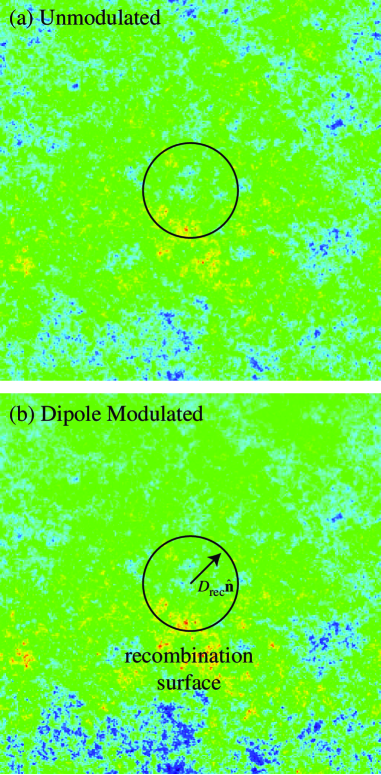
The two point correlation of the model in terms of the power spectra of the fields and was given in Gordon et al. (2005) and is rederived in our framework of 3D fields in §A.1. In this framework, the modulation appears as the product of the Gaussian random field and the modulation field to form the observed temperature field. For the temperature field, this is equivalent to the product of the 2D angular fields projected onto the recombination surface (see Fig. 1, solid circle). Likewise the two point correlation can be expressed in terms of operations on the angular power spectra of the and fields in projection. We shall now see that these simplifications do not carry over to the polarization field.
II.3 Polarization Field
Broken homogeneity and isotropy are also transferred onto the CMB polarization field. A modulation model that is designed to explain temperature anomalies can be tested through the predictions it makes for polarization.
Large-angle polarization is generated by the rescattering of photons off free electrons during the reionization epoch. A quadrupole anisotropy in the temperature of the radiation leads to linear polarization of the CMB. More specifically, from the temperature field at recombination of Eq. (5), the quadrupole moments at each position in space are given by
| (9) |
Note that describes a set of 5 three dimensional source fields. Furthermore the angular integral is over the recombination surface of an (electron) observer at position a distance away from the true observer at the origin
| (10) |
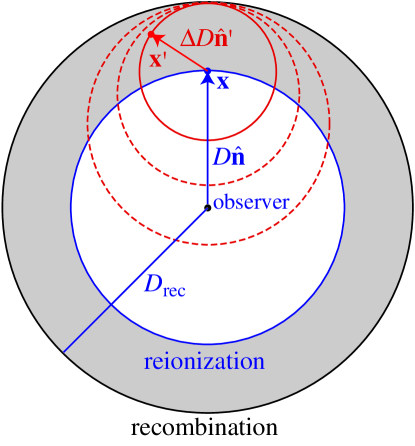
where is the radius of recombination surface of the electron, as illustrated by Fig. 2.
To the true observer at the origin, scattering at position generates a contribution to the Stokes parameters of the polarization in direction given by Hu (2000)
| (11) | |||||
where are the spin spherical harmonics and is the optical depth between a comoving distance and the present epoch. When we specify without the argument , we refer to the total optical depth to reionization. The analogue of temperature multipole moments for linear polarization are the and multipole moments
| (12) |
and modes are the tensor analogues of curl-free and divergence free components of a vector. An -mode has a polarization direction that is aligned with or orthogonal to the direction that the mode amplitude changes. A -mode has this direction rotated by . When polarization is generated by a scalar field, only -modes are formed. In Fourier space, this property is easily seen since the polarization direction from each mode must follow the direction of itself. Since the modulation preserves the scalar nature of the source of polarization, -modes are absent even in the modulated case. Note that this is different from a direct modulation of the polarization amplitude itself by a scalar quantity, e.g. from spatial fluctuations in Hu (2000). In that case, the polarization direction is fixed by the potential field from recombination but the amplitude carries additional directionality from the modulation.
Predictions for the modulated polarization field, unlike the temperature field, require a 3D model of the modulation. Eq. (10) implies that the relevant modulation is at position in a sphere around each source at position for each angular position (see Fig. 2). Furthermore, these sources lie in the interior of the recombination surface of the temperature field. Likewise the polarization statistics cannot be expressed as an operation on the angular power spectra of the fundamental and fields corresponding to a single projection. The analytic framework for predicting the two point correlations is given in §A.2. Given the cumbersome nature of this framework, we instead rely on numerical simulations to study modulated statistics as we shall now describe. We use the analytic framework to test these simulations (see §A.3) and to provide insight on statistical quantities that should be measured in the simulations and data (see §A.4).
II.4 Simulations
Numerical simulations are conceptually the simplest and most general way of assessing the statistics of the modulated temperature and polarization fields.
We first simulate the 3D potential field by combining realizations of the two Gaussian random -fields with the deterministic modulation field . We typically chose the length of the periodic box to be four times the diameter of the recombination surface with pixels. This ratio of sizes and dynamic range allows us to cover the scales of interest in this work.
To obtain the temperature field, we then interpolate the field onto a 2D surface of radius and weight it according to the Sachs-Wolfe relation (5). Finally we use the HEALPix package Gorski et al. (2005) to extract the multipole moments of the field. The interpolation is done in every unit vector corresponding to HEALPIX pixel centers at resolution . As an example, slices through simulations of unmodulated and dipole-modulated temperature fields are shown in Fig. 1. The statistics of these temperature simulations match those of the 2D approach where the modulation is directly in angular space on the recombination surface. We will occasionally use 2D simulations where only the temperature field is required and for unmodulated cases to build large samples.
The polarization field is equally straightforward to simulate but numerically more involved. We take the same 3D simulations employed for the temperature field and compute the quadrupolar temperature sources for redshifts in equal steps along each line of sight, and in every unit vector corresponding to HEALPIX pixel centers at resolution around the sky. Then, we generate maps of polarization by means of Eq. (11). Once the maps are created, the coefficients are obtained using the HEALPix package Gorski et al. (2005), and various polarization statistics described below are computed.
We test this pipeline against analytic calculations of unmodulated and simple modulation models in §A.3. It is the main tool used to assess the temperature and polarization statistics in this work. It can be used for arbitrarily complicated modulation fields and any statistical property of the temperature and polarization fields.
III Dipolar Modulation
Eriksen et al. Eriksen et al. (2004) showed that there is a hemispherical or dipole asymmetry in the amount of power in the WMAP data at multipoles . The axis of this asymmetry points in a direction that is close to the South Ecliptic Pole (SEP) making the power in the southern hemisphere larger than the north. It was subsequently pointed out that a dipolar modulation of the form of Eq. (32) with a modulation field of
| (13) |
could explain the asymmetry though not the curious alignment with the SEP Spergel et al. (2003); Gordon (2007); Eriksen et al. (2007). Note that in a coordinate system where the -axis points along the modulation axis. We set the field to have power only at and hence its contribution is irrelevant in our considerations. We take the field to have a scale invariant power spectrum
| (14) |
with which corresponds to the WMAP 3-year normalization for a cosmology with matter density , cosmological constant , baryon density , Hubble constant km s-1 Mpc-1, and spatially flat spatial geometry.
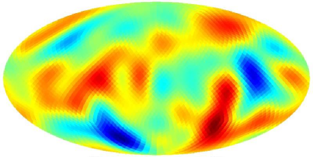
Once is specified, we can use our simulation pipeline to make realizations of the polarization field. An extreme example with is shown in Fig. 3. Note that the hemispherical power asymmetry carries through to the polarization.
The WMAP temperature field however suggests a much weaker dipole modulation that can only be detected statistically in the polarization. We will base our parameter choices on the analysis of Ref. Eriksen et al. (2007) which found with excluded at the 99% CL. For illustrative purposes we will take a reionization model with where hydrogen is fully ionized out to a maximum redshift and neutral thereafter. We test sensitivity to the reionization history in §III.2.
III.1 Dipole Modulation Statistics
The dipolar modulation in the potential field gives rise to couplings between and multipole moments in not only
| (15) |
but also in all of the two point combinations involving
| (16) |
specifically . We derive the proportionality coefficients in Appendix A.4. Each multipole pair then forms a noisy estimator of the dipole modulation parameter . Even in the absence of detector noise and foregrounds, the cosmic variance of the temperature and polarization fields provide noise to the measurement. Eqs. (84) and (85) give the unbiased minimum variance combinations of the multipole pairs as estimators of .
The first question we ask is: if the observed dipole asymmetry at is a statistical fluke and that the true ensemble average is , how well can temperature and polarization at rule out a finite value of near the best fit of ? Under this assumption, we show the distribution of the estimators and the joint estimator in Fig. 4. These distributions were generated from 2D simulations of the unmodulated temperature and polarization fields in accordance with the power spectra of Eq. (A.1), (65) and (75).
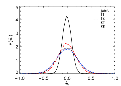
Given alone, the hypothesis that can only be weakly tested. Specifically, a value of can be tested at the confidence level (CL) by . Each of the polarization estimators can in principle test dipole modulation at a comparable level: can be tested at confidence by , at CL by and at CL by . The combination of the four estimators however is more powerful: can be tested at CL by the joint estimator. For reference, the central value of Eriksen et al. (2007), , yields a 99.3% CL test. Furthermore the upper limit on achievable with the joint estimator is .
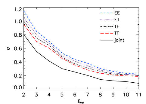
Most of the polarization information comes from multipoles in the range of . In Fig. 5 we show the rms fluctuation in the estimators as a function of , the maximum multipole employed in the estimators. Note that the estimators involving polarization saturate by .
The next question we ask is: given a true model of , how well can an isotropic model of be excluded? Fig. 6 shows the distribution of coming from realizations of a 3D modulated model (histogram, ). In these simulations occurred in less than of the realizations. Furthermore the mean of the samples is consistent with being unbiased and the standard deviation is consistent with the expectations from Fig. 5.

III.2 Model Dependence and Noise
These tests are only weakly sensitive to the assumed reionization history for a cosmic variance limited observation. The main difference is that a linear modulation produces a weaker effect for nearby sources of polarization and hence the signal decreases with . As an example, we calculate the level of detectability for an unphysically small optical depth of . Even for this extreme case, values of are ruled out at the CL by the joint estimator. An intermediate case of rules out values of at the CL.
Because most of the signal comes from low multipoles in the polarization , the cosmic variance limit described in the previous section is within the statistical reach of the Planck satellite. For definiteness we take the and frequency channels and combine them into an effective white noise power spectrum of K-arcmin at low multipoles. Noise in the temperature field is negligible compared with cosmic variance. Quantitatively, for a reionization history with optical depth , and the noise level considered for Planck, values of are ruled out at CL by the joint estimator . A space-based experiment with no foregrounds, frequency channels and a noise level of K-arcmin per frequency channel would essentially saturate the cosmic variance bound in each channel. Given these results, foregrounds and systematics will probably be the limiting factor in how well dipole modulation can be tested by polarization. We leave this subject to a future work.
Finally, the model spectrum assumes that the temperature anisotropy comes purely from the Sachs-Wolfe effect. A CDM model would predict that the ensemble averaged quadrupole has a substantial contribution from the so-called Integrated Sachs-Wolfe (ISW) effect from the decay of potentials during the acceleration epoch. Under CDM, the measured low power quadrupole anisotropy could indicate that either the ISW contributions to the quadrupole are by chance small on our sky or that there is a chance cancellation between the two contributions. Finally, it could indicate an alternate model of the dark energy where the ISW contributions are smaller Caldwell et al. (1998); Hu (1998); Bean and Dore (2004) or designed to cancel the Sachs-Wolfe effect Gordon and Hu (2004). In all of these explanations, the polarization field is unaffected.
Nonetheless, the dipole modulation tests involving the temperature field are slightly weakened if the ISW contributions to CDM are added back as a source of noise. Correspondingly the joint estimators also weaken. For example, for a reionization model with optical depth the joint estimator can test values of at the CL.
In summary, prospects for future polarization tests of dipole modulation at the level at the 98% CL are fairly robust to model assumptions.
IV Quadrupolar Modulation
de Oliveira-Costa et al. de Oliveira-Costa et al. (2004) pointed out that there are several striking features of the temperature dipole, quadrupole and octopole in the WMAP data. The octopole is highly planar and defines a preferred axis that is near the dipole axis. Moreover the quadrupole is also weakly planar in the same coordinate system.
Gordon et al. Gordon et al. (2005) subsequently showed that a quadrupolar modulation with a preferred axis that is by chance near the dipole direction can make these features substantially more likely. Specifically, we will take a modulation to the potential field of the form of Eq. (1), with
| (17) |
Note that the -axis required here is not the same as in the dipole modulation case. Since , this introduces a quadratic term to the spatial modulation.
These anomalies are confined to the low multipoles and so the modulation must also be confined to low multipoles. For the angular modulation considered in Gordon et al. (2005), this was simply imposed as a sharp suppression in multipole space of the field. Spatial modulation is more complicated in that even a sharp suppression in Fourier space is broadened by projection effects. Given these considerations, we take a two field model defined by
| (18) | |||||
| (19) |
where the normalization is given as in the dipole modulation model by the WMAP normalization. We introduce a scaling parameter that controls the amount of power at low relative to this normalization. We begin our analysis by finding regions in the parameter space of that maximize the probability of the observed quadrupole-octopole alignment.
IV.1 Maximizing Temperature Alignments
To quantify the quadrupole-octopole alignment, de Oliveira-Costa et al. de Oliveira-Costa et al. (2004) introduced the normalized angular momentum along a given axis
| (20) |
where the are the multipole moments of the temperature field in that preferred frame. More specifically, from the moments defined in galactic coordinates , the rotated ones are
| (21) |
where the Euler angles are , , and and is the Wigner rotation matrix Copi et al. (2004); Gordon et al. (2005). Note that is invariant under the final rotation by .
In particular, the statistic
| (22) |
captures both the alignment between the quadrupole and octopole, and the planarity of the octopole. The preferred axis is then chosen as the one which maximizes this statistic. For the ILC map of the 3-year WMAP data corrected for the kinematic quadrupole, . This is slightly smaller than for the 1-year WMAP data in the TOH map Tegmark et al. (2003), used in previous studies: Copi et al. (2004); Gordon et al. (2005). For an unmodulated model, occurred in only of 2D realizations.
Quadrupole modulation can dramatically increase the probability of a high angular momentum statistic. To find the parameters that maximize this probability, we first vary the parameters with and find the set that gives maximum number of realizations with . Taking eliminates the contributions from the unmodulated field that could otherwise destroy alignments at low multipoles. The alignment probability then is also independent of .
We then generate 2D Monte Carlo (MC) realizations for each of the modulated models. For each realization, the estimator is computed on a grid of positions on the celestial sphere by performing the rotation of in Eq. (21). Taking the maximum value of attained for each realization, we compute for each model the percentage of realizations with .
The region of parameter space that corresponds to the highest alignments is centered around , in agreement with Gordon et al. (2005). Furthermore, wavenumbers that best project onto a multipole correspond to ; more specifically for the region that best projects onto the quadrupole and octopole at the distance to recombination. Furthermore keeping and in a narrow range around this value eliminates contamination from the modulation of longer and shorter wavelengths in the quadrupole and octopole.
For definiteness, we take , and though any would produce similar results due to unavoidable projection effects. With this choice, of realizations have . This number is smaller than that quoted in Gordon et al. (2005) due to these projection effects but is still a factor of larger than the probability in unmodulated models.
While taking maximizes alignments, it does not provide for a realistic model. The absence of high wavenumbers would be in conflict with the observed fluctuations at higher multipole moments. This is exhibited in a poor ILC likelihood
| (23) |
where is the element vector of observed values and is their signal plus noise covariance matrix. To remedy this problem we keep the first field fixed to the parameters above but add in the second field at a finite and maximize the likelihood over their relative amplitude .

Fig. 7 (lower panel) shows the dependence of on for relative to CDM (see below Eq. (14)). Decreasing this parameter creates a better fit to the data at the expense of decreasing the probability of the quadrupole-octopole alignment (upper panel). As a compromise we choose a model with that neither improves nor worsens the fit. The model parameters then become
| (24) |
for which the probability of is (see Fig. 8).
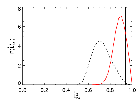
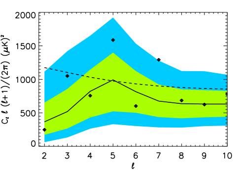
Fig. 9 shows the temperature angular power spectrum of this model along with the WMAP 3-year temperature data for the first multipoles. The bands shown here represent the and cosmic variance confidence regions for this model taken from 2D realizations of the temperature field. Note that the cosmic variance is larger for the modulated model due to the -dependence of the power.
In Fig. 10 we show a realization of the model that has a high normalized angular momentum , shown in the frame of the modulation, illustrating how the modulation takes a random isotropic sky and aligns the quadrupole and the octopole.

IV.2 Polarization Angular Momentum
With the quadrupolar modulation model set by Eq. (IV.1) to maximize temperature alignments and fit the WMAP temperature data, we can now use our simulations to make polarization predictions.
We first examine the normalized angular momentum statistic of the polarization field. We define this statistic in the same way as for the temperature field
| (25) |
with the combined quadrupole and octopole statistic being
| (26) |
There is one important difference between this statistic and the temperature based one. In the case of polarization predictions, the temperature field has already defined the preferred axis against which we should measure the polarization angular momentum. Consequently, no search over directions is required.
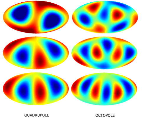
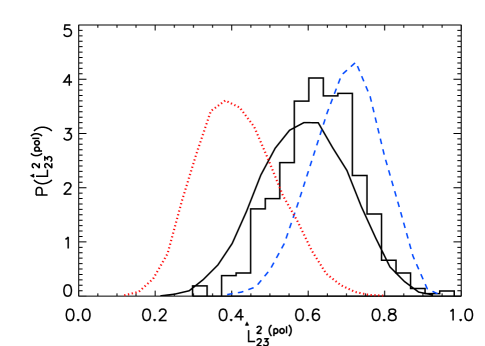
Fig. 11 shows a histogram of for out of 3482 3D realizations of the modulated model that have as high or higher temperature alignment than WMAP . We first compare this with the same statistic for 2D isotropic realizations of an unmodulated polarization field (red dotted line). There is a tendency for the polarization field to be aligned compared with random isotropic realizations. An example of a typical realization is shown in Fig. 12 (second row) and is to be compared with a typical isotropic realization (first row). Note the similarity between temperature alignments and polarization aligments in Figs. 10 and 12. Both have a deficit of power near the poles in the frame of the modulation. However the polarization amplitude is in fact the largest at the poles. In this direction, the electron scattering sees the planar quadrupole in the transverse plane and scatters it into a maximal polarization. Foregrounds which have high polarization where there is high intensity will not have this pattern.
However, the expected correlation between the temperature and polarization fields implies that there should be some tendency for polarization alignment in any explanation in which the alignment of the temperature field reflects contributions from the recombination surface, and not a foreground, secondary or systematic effect. This includes an isotropic unmodulated model in which the temperature alignment is a chance occurrence.
To quantify this tendency, we consider two isotropic models which have been conditioned to have for the temperature field. More specifically, we draw a polarization field that is consistent with the observed temperature field and model power spectra,
| (27) |
where is a complex Gaussian variate of zero mean with and .
The first is the Sachs-Wolfe model where all of the temperature anisotropy arises from recombination. Under this assumption, the temperature alignments are a real feature of the recombination surface and the ISW effect in our local universe happens to be small in the quadrupole and octopole. Fig. 11 (blue dashed lines) shows the polarization statistic for 2D constrained realizations of this model. An example of a highly aligned realization is shown in Fig. 12 (third row).
Compared with the modulated model, there is an even higher probability of polarization alignment here. The reason is that in the former, the strength of the spatial modulation increases as the square of the distance. The closer distance to reionization implies a substantially weaker modulation of the polarization field as compared with the temperature field. Ironically, a very high value of would strongly disfavor the modulated model compared with the isotropic Sachs-Wolfe model. The upper limit for the modulated model is .
It is also possible that the alignment of the quadrupole and octopole does not represent an aligned spatial configuration at all and is instead the result of a chance combination of the Sachs-Wolfe effect and ISW effects. These effects arise from very different physical scales but are seen in projection at the same angular scale. To illustrate this case, we draw 2D realizations of the CDM model (see below Eq. (14)) that are similarly conditioned to have for the temperature field. The histogram of the polarization statistic is shown in Fig. 11 (black solid curve). The presence of a temperature contribution that does not correlate with polarization shifts the distribution downwards and decreases the probability of polarization alignments. The distribution is still distinct from the truly random isotropic simulations (red dotted lines). The 95% lower limit on this model is .
The final possibility is that the temperature quadrupole and temperature field is nearly all local secondary anisotropy and that the Sachs-Wolfe effect is anomalously low (e.g. Vale (2005); Inoue and Silk (2006)). The polarization distribution would then look like the truly random isotropic simulations (see Fig. 11, red dotted line). In this case, the polarization amplitude itself would also be anomalously low.
In summary, a very low value of with a normal polarization amplitude would suggest that the origin of the temperature alignments is not cosmological. A very low value with suppressed polarization amplitude would imply a purely secondary origin to the temperature alignment. A very high value would rule out the modulated model and also imply that the ISW effect is nearly absent in the WMAP low multipoles.
IV.3 Quadrupole Modulation Statistics
Beyond the angular momentum of the quadrupole and octopole, a quadrupolar modulation model makes further testable predictions. These predictions however are more sensitive to the choice of model parameters.
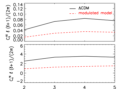
First, the angular power spectrum of the polarization and temperature cross correlation differs in its relationship to the temperature power spectrum due to the modulation. In Fig. 13, we show these spectra for the model of Eq. (IV.1). Note that for the same optical depth , the polarization spectra have less power. This is a consequence of the decrease in modulation amplitude at the closer distance to reionization. Unfortunately, this signature is largely degenerate with a change in the optical depth and so is not a unique signature of modulation.
Similar to dipole modulation, quadrupole modulation generates a more unique signature in the correlation between neighboring multipole moments
| (28) |
where . In our two field model, most of the modulation is confined to the low multipoles and so the signal is mainly in . Note that an isotropic model that by chance has quadrupole-octopole temperature alignments will still predict a zero expectation value for these quantities.
Let us define a correlation statistic
| (29) |
which tests the phase alignment of the moments and takes on values from . In the absence of modulation, these statistics have zero mean but any given pair has large cosmic variance. Given a modulation model that predicts
| (30) |
we can construct a weighted sum
| (31) |
where . This statistic has the property that its expectation value is zero for an isotropic field and for the chosen modulation model.
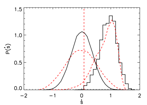
We begin by considering the case and the modulated model of Eq. (IV.1) as in the previous section. The distribution of is shown in Fig. 14 (dashed lines, right curve) from 2D simulations. The WMAP ILC data has and disfavors the modulated model but not at high significance: of the modulated simulations have less than the data. Conversely the data would be a typical realization of an isotropic model (see Fig. 14, dashed lines, left curve). Likewise an occurred in of the modulated simulations, and an occurred in of the isotropic simulations. These two tails of the respective distributions represent the power of the statistic to distinguish typical realizations of the models.
The addition of polarization information would make these tests definitive by reducing the probability in the tails (see Fig. 14, solid curves). When all fields are considered , the probabilities in the tails drop to in only of the modulated 3D simulations and in of the 2D isotropic simulations. The latter probability assumes a Sachs-Wolfe only model for the temperature field. If the ISW contribution of CDM is factored in, the probability increases slightly to .
Consequently a quadrupolar modulation with parameters given by Eq. (IV.1) will be definitively tested through the statistic by polarization measurements that approach the cosmic variance limit for . However a model with a lesser amount of modulation at may evade such constraints. The amount of modulation in these multipoles is controlled by and hence mainly constrains this parameter. In the model we have been considering, . Lowering this value increases the contribution of the unmodulated field for . But the price is to make the quadrupole-octopole alignment less likely (see Fig. 7).
As a specific example, for and , the probability of decreases from 16.6% to 10% (see Fig. 7). On the other hand, it improves the fit to the WMAP data by making relative to CDM. Correspondingly, the -statistic also weakens in its discriminating power. For the case, the WMAP ILC data has . For this case, of simulations have a smaller value of . Similarly, a value of occurred in of the modulated simulations, and occurred in of the isotropic simulations. With the addition of polarization information these tests become more significant: only occurred in only of the modulated simulations and only occurred in in of the isotropic simulations.
In summary, while the -statistic cannot rule out quadrupolar modulation in general, it can severely limit the amount of modulation allowable at and hence test its ability to explain the quadrupole-octopole alignment.
V Discussion
Statistical anomalies in the large-scale CMB temperature sky measured by WMAP have been suggested as possible evidence for the violation of statistical isotropy on large scales. In any physical model for such a violation, there are testable consequences for the CMB polarization field.
We have developed a radiative-transfer simulation-based approach to predicting these consequences. We have applied this approach to modulation models of broken isotropy. In this class of models, a long-wavelength modulation of shorter-wavelength fluctuations breaks isotropy locally, while the universe remains globally isotropic and homogeneous.
A linear or dipolar modulation can be used to explain the observed power asymmetry between the northern and southern ecliptic hemispheres at multipole moments Eriksen et al. (2004); Spergel et al. (2003); Gordon (2007); Eriksen et al. (2007). Linear modulation produces a dipole coupling that correlates multipole moments to in all of the two point functions of the temperature and polarization field. Using an analytic framework developed in the Appendix, we derive an estimator of the modulation amplitude from these fields from these correlations.
We find that the addition of polarization information substantially improves the ability to test for dipole modulation at the lowest multipoles . Under a wide range of assumptions, the dipole modulation explanation of the hemisphere asymmetry can be tested at the 98% CL or greater. These tests will require near cosmic variance limited polarization measurements at the low multipoles. Such measurements are within the statistical reach of the Planck satellite but systematic contamination from foregrounds will have to be sufficiently controlled.
A quadratic or quadrupolar modulation in the temperature field can be used to explain the alignment of the quadrupole and octopole de Oliveira-Costa et al. (2004); Gordon et al. (2005). We generalize the considerations of Ref. Gordon et al. (2005) and develop full 3D models that enhance the probability of alignments by a factor of .
These models predict that the quadrupole and octopole of the -polarization will tend to align as well. However alignment of the polarization mainly tests that the temperature alignment is cosmological and originates from recombination, not the specifics of the modulation model. As such its main use will be to reject explanations of the alignments due to foregrounds or purely local secondary anisotropy. In fact a very high alignment, comparable to the temperature field, is not expected in the modulation model due to the smaller strength of the modulation at the distance to reionization. If such an alignment is seen then it is more likely that it arises from a chance configuration of the temperature field at recombination.
Quadrupolar modulation models can be distinguished in a manner similar to the dipole modulation but through a correlation between multipoles and in the temperature and polarization fields. We find that the combination of temperature and polarization information out to can strongly constrain the level of modulation in the low multipoles. As a consequence, polarization measurements can in principle rule out models that make the temperature alignments more than a few percent likely CL or stronger.
In general, matching signatures of broken isotropy in the polarization provide a powerful test of competing explanations of the temperature anomalies. Explanations that involve foregrounds (e.g. Slosar and Seljak (2004)) or local gravitational effects Inoue and Silk (2006); Vale (2005) would tend to predict different signatures. This is especially true since matching anomalies in the polarization are non-local in the Stokes parameters. Possible experimental systematics would be specific to a given experiment, and would thus have to be analyzed in a case by case basis. Therefore we do not consider them in this paper.
The examples we have studied illustrate that polarization in the future will provide a fruitful testing ground for explanations of the observed temperature anomalies. As predictions of anomaly models, polarization statistics move beyond the a posteriori inferences that currently dominate the field.
Acknowledgements.
We thank Alexander Belikov, Colin Bischoff, Olivier Dor, Christopher Gordon, Gary Hinshaw, Dragan Huterer, Michael Mortonson, Kendrick Smith, and Glenn Starkman for useful discussions. We acknowledge use of the HEALPIX package and the Legacy Archive for Microwave Background Data Analysis (LAMBDA). This work was supported by the KICP through the grant NSF PHY-0114422. HVP was additionally supported by NASA through Hubble Fellowship grant #HF-01177.01-A awarded by the Space Telescope Science Institute, which is operated by the Association of Universities for Research in Astronomy, Inc., for NASA, under contract NAS 5-26555. WH was additionally supported by the DOE through contract DE-FG02-90ER-40560 and the David and Lucile Packard Foundation.Appendix A Analytic Modulation Framework
In this Appendix, we construct an analytic framework for modulated temperature (§A.1) and polarization statistics (§A.2) and evaluate them explicitly for dipole modulation. We use these analytic calculations to cross check numerical results in §A.3 and to construct estimators of the dipole modulation in §A.4.
A.1 Modulated Temperature Field
For the temperature field, the effect of modulation can be viewed as either the direct projection of the modulated (convolved in Fourier space) field or the convolution in harmonic space of the multipole moments of the original fields. The latter perspective is taken in Ref. Gordon et al. (2005) for the temperature field. We show in this section that the former is equivalent and more closely resembles the derivation required for polarization in §A.2.
For notational simplicity, we will derive the contribution to the spectrum due only to the modulated piece of the model of Eq. (1) so that
| (32) |
The unmodulated piece can be added to these results without loss of generality.
The Fourier moments of are given by a convolution of the two fields and ,
| (33) |
and the two point function of the field becomes
| (34) | ||||
Under the Sachs-Wolfe approximation of Eq. (5), the spherical harmonic decomposition of the temperature field yields
| (35) |
which implies a two-point function of the temperature harmonics of
| (36) | |||||
Eqs. (A.1) and (36) provide the analytic framework for modulated temperature two-point statistics.
To make these considerations concrete, let us explicitly evaluate Eq. (36) for dipole modulation. Dipole modulation can be taken to be a local approximation to a superhorizon scale Fourier mode,
| (37) | |||||
where we choose . The Fourier representation of the field becomes
| (38) |
Now let us substitute this expression into Eq. (A.1). The first term is zeroth order in and is just the standard angular power spectrum
| (39) |
where
The second term is first order in and is given by
The simplification of these expressions requires to be expressed in terms of where . Assuming that , we can expand,
| (40) |
where the coupling matrix is defined as 222The normalization differs from Ref. Gordon et al. (2005) by .
| (45) |
With these relations, the first order term in becomes
| (46) |
By virtue of the Wigner 3 symbol in the coupling matrix, the dipole modulation couples to with a strength that is linear in or .
Likewise, the same operations on the term quadratic in yield
| (47) |
The quadratic term in or couples to . These results are the same as obtained in Ref. Gordon et al. (2005).
A.2 Modulated Polarization Field
For predicting polarization statistics, the direct angular modulation approach of Gordon et al. (2005) does not apply given that the sources of the polarization field are modulated and not the field itself.
The quadrupole source comes from the temperature field through Eq. (9)
| (48) |
where recall (see Fig. 2).
Decomposing into Fourier modes yields
| (49) |
The Stokes parameters of the polarization are given by Eq. (12)
| (50) | |||
Recoupling the last line of Eq. (50), we have
| (55) | |||
| (56) |
Decomposing into the spin-2 spherical harmonics,
| (57) | |||
| (62) |
Note that the -modes vanish since the second Wigner symbol is zero if is odd and
| (63) |
This is to be expected since all scalar sources, even products of fundamental scalars, generate only -modes.
Paralleling the modulated temperature derivation of §A.1, we find that there is the zeroth order piece coming from the unmodulated field that reproduces the standard result Hu and White (1997).
| (64) |
where
| (65) |
with
| (66) |
and the polarization radial function
| (67) |
The linear piece in of the dipole modulation becomes
| (68) |
Assuming, as in the temperature case, that , we can again Taylor expand the spherical Bessel functions and the spherical harmonic which, after some algebra, reduces Eq. (A.2) to
| (69) |
where
| (70) |
and
| (71) |
with defined in Eq. (66). Like the temperature field, the coupling of to is linear in . The quadratic term can be similarly calculated but is more cumbersome and we omit the derivation here.
For reasonable reionization histories, the dominant term in Eq. (A.2) is the first term. Comparing Eq. (65) with (A.2) we see that to order of magnitude,
| (72) |
where is a typical distance to reionization. Compared with the modulation of the temperature spectrum in Eq. (46), the modulation of the polarization spectrum is suppressed by a factor of . This factor is due to the lower level of spatial modulation at typical distances to reionization in the dipolar model of Eq. (37). Typically, it has a value of .
For the two point function, the same operations yield
| (73) |
with
| (74) |
where is the usual unmodulated cross power spectrum
| (75) |
and is defined in Eq. (66).
A.3 Comparison with Simulations
In this section, we test the 3D simulation method against the analytic results of §A.1 and A.2. The simulations are performed according to the algorithm described in Section II.4 with a box of size that is four times the diameter of the last scattering surface and a spatial resolution defined by the pixels.
We first test the simulations against the usual results given by Eq. (A.1), (65), and (75) for an unmodulated scale invariant potential spectrum. The temperature power spectra averaged over multiple realizations agrees with the analytic results within the sample variance
| (76) |
where is the number of simulated skies.
In order to predict the -modes, we calculate the quadrupolar temperature sources for radii along each line of sight, and in every unit vector corresponding to HEALPIX pixel centers at resolution . The small evolution of perturbations of the potential field between recombination and reionization is accounted for via the transfer function.
We compute the modes for different reionization histories with ionization fraction equal to out to a redshift where the optical depth and zero beyond this redshift. In all cases, the distribution of numerical spectra are consistent with cosmic variance for . For larger multipoles there is a diminution of power that is consistent with the Nyquist frequency of the box, but this does not affect any of our results.
Finally, we check the dipole modulation model against the analytic results of the previous sections. We showed there that a dipole modulation gives rise to couplings between and modes in the , , and two point functions. As an example of these correlations, we compare simulation results with the analytic calculation in Fig. 15. We again find agreement within sample variance expectations.

A.4 Dipolar Modulation Estimators
From the analytic calculations of §A.1 and A.2, we can construct unbiased estimators of the dipole modulation amplitude . In the presence of a dipole modulation, the expectation values of temperature and polarization modes and are correlated. Each pair of multipoles then forms an estimator of
| (77) |
where , are coupling matrices defined in Eq. (A.1) and the coefficients are given by
| (78) |
such that . Specifically, Eqs. (46), (A.2), and (A.2) give
| (79) | ||||
Each estimator carries a large sample variance and so one can combine them to form the joint estimator
| (80) |
where are the weights assigned to each one. To maintain the condition that the estimator is unbiased , the weights must satisfy
| (81) |
Note that while individual estimators are complex, the joint estimator is real if and are combined with equal weights.
We employ weights that minimize the variance of the joint estimator. Given a model with , the variance is
| (82) |
Here are the components of the matrix given by
| (83) |
where are the standard angular power spectra coefficients.
Imposing the normalization constraint on the weights, given by Eq. (81), we minimize the variance with
| (84) |
which is the usual inverse covariance weight of covarying estimators. Likewise in the case that just one of the combinations is used this general form reduces to
| (85) |
which is the usual inverse variance weighted estimator. Note that the sum over can be restricted to for modulation models which only affect large scales.
Finally, given instrumental noise power spectra , the variance and minimum variance weights are modified by including the spectrum into the covariance matrix
| (86) |
where we typically assume that the noise cross power spectrum vanishes.
References
- Bennett et al. (2003) C. L. Bennett et al. (WMAP), Astrophys. J. Suppl. 148, 1 (2003), eprint astro-ph/0302207.
- Spergel et al. (2003) D. N. Spergel et al. (WMAP), Astrophys. J. Suppl. 148, 175 (2003), eprint astro-ph/0302209.
- Hinshaw et al. (2006) G. Hinshaw et al. (WMAP) (2006), eprint astro-ph/0603451.
- Page et al. (2006) L. Page et al. (WMAP) (2006), eprint astro-ph/0603450.
- Eriksen et al. (2004) H. K. Eriksen, F. K. Hansen, A. J. Banday, K. M. Gorski, and P. B. Lilje, Astrophys. J. 605, 14 (2004), eprint astro-ph/0307507.
- de Oliveira-Costa et al. (2004) A. de Oliveira-Costa, M. Tegmark, M. Zaldarriaga, and A. Hamilton, Phys. Rev. D69, 063516 (2004), eprint astro-ph/0307282.
- Land and Magueijo (2005a) K. Land and J. Magueijo, Mon. Not. Roy. Astron. Soc. 362, 838 (2005a), eprint astro-ph/0502574.
- Tegmark et al. (2003) M. Tegmark, A. de Oliveira-Costa, and A. J. S. Hamilton, Phys. Rev. D 68, 123523 (2003).
- Copi et al. (2004) C. J. Copi, D. Huterer, and G. D. Starkman, Phys. Rev. D70, 043515 (2004), eprint astro-ph/0310511.
- Schwarz et al. (2004) D. J. Schwarz, G. D. Starkman, D. Huterer, and C. J. Copi, Phys. Rev. Lett. 93, 221301 (2004), eprint astro-ph/0403353.
- Land and Magueijo (2005b) K. Land and J. Magueijo, Phys. Rev. Lett. 95, 071301 (2005b), eprint astro-ph/0502237.
- Eriksen et al. (2007) H. K. Eriksen, A. J. Banday, K. M. Gorski, F. K. Hansen, and P. B. Lilje, Astrophys. J. 660, L81 (2007), eprint astro-ph/0701089.
- Copi et al. (2006) C. J. Copi, D. Huterer, D. J. Schwarz, and G. D. Starkman, Mon. Not. Roy. Astron. Soc. 367, 79 (2006), eprint astro-ph/0508047.
- Copi et al. (2007) C. Copi, D. Huterer, D. Schwarz, and G. Starkman, Phys. Rev. D75, 023507 (2007), eprint astro-ph/0605135.
- Wiaux et al. (2006) Y. Wiaux, P. Vielva, E. Martinez-Gonzalez, and P. Vandergheynst, Phys. Rev. Lett. 96, 151303 (2006), eprint astro-ph/0603367.
- Land and Magueijo (2005c) K. Land and J. Magueijo, Mon. Not. Roy. Astron. Soc. 357, 994 (2005c), eprint astro-ph/0405519.
- Magueijo and Sorkin (2007) J. Magueijo and R. D. Sorkin, Mon. Not. Roy. Astron. Soc. Lett. 377, L39 (2007), eprint astro-ph/0604410.
- Land and Magueijo (2007) K. Land and J. Magueijo, Mon. Not. Roy. Astron. Soc. 378, 153 (2007), eprint astro-ph/0611518.
- Gordon and Trotta (2007) C. Gordon and R. Trotta (2007), eprint arXiv:0706.3014 [astro-ph].
- Hajian and Souradeep (2003) A. Hajian and T. Souradeep, Astrophys. J. 597, L5 (2003), eprint astro-ph/0308001.
- Hajian and Souradeep (2006) A. Hajian and T. Souradeep, Phys. Rev. D74, 123521 (2006), eprint astro-ph/0607153.
- Donoghue and Donoghue (2005) E. P. Donoghue and J. F. Donoghue, Phys. Rev. D71, 043002 (2005), eprint astro-ph/0411237.
- Armendariz-Picon (2006) C. Armendariz-Picon, JCAP 0603, 002 (2006), eprint astro-ph/0509893.
- Basak et al. (2006) S. Basak, A. Hajian, and T. Souradeep, Phys. Rev. D74, 021301 (2006), eprint astro-ph/0603406.
- Pullen and Kamionkowski (2007) A. R. Pullen and M. Kamionkowski, Phys. Rev. D76, 103529 (2007), eprint arXiv:0709.1144 [astro-ph].
- Gordon et al. (2005) C. Gordon, W. Hu, D. Huterer, and T. Crawford, Phys. Rev. D72, 103002 (2005), eprint astro-ph/0509301.
- Gordon (2007) C. Gordon, Astrophys. J. 656, 636 (2007), eprint astro-ph/0607423.
- Sachs and Wolfe (1967) R. Sachs and A. Wolfe, Astrophys. J. Suppl. 147, 73 (1967).
- Hu (2000) W. Hu, Astrophys. J. 529, 12 (2000), eprint astro-ph/9907103.
- Gorski et al. (2005) K. M. Gorski et al., Astrophys. J. 622, 759 (2005), eprint astro-ph/0409513.
- Caldwell et al. (1998) R. R. Caldwell, R. Dave, and P. J. Steinhardt, Phys. Rev. Lett. 80, 1582 (1998), eprint astro-ph/9708069.
- Hu (1998) W. Hu, Astrophys. J. 506, 485 (1998), eprint astro-ph/9801234.
- Bean and Dore (2004) R. Bean and O. Dore, Phys. Rev. D69, 083503 (2004), eprint astro-ph/0307100.
- Gordon and Hu (2004) C. Gordon and W. Hu, Phys. Rev. D 70, 083003 (2004), eprint astro-ph/0406496.
- Vale (2005) C. Vale (2005), eprint astro-ph/0509039.
- Inoue and Silk (2006) K. T. Inoue and J. Silk, Astrophys. J. 648, 23 (2006), eprint astro-ph/0602478.
- Slosar and Seljak (2004) A. Slosar and U. Seljak, Phys. Rev. D70, 083002 (2004), eprint astro-ph/0404567.
- Hu and White (1997) W. Hu and M. J. White, Phys. Rev. D56, 596 (1997), eprint astro-ph/9702170.