Detection of Contact Binaries Using Sparse High Phase Angle Lightcurves

Abstract

We show that candidate contact binary asteroids can be efficiently identified from sparsely sampled photometry taken at phase angles $\alpha>60$°. At high phase angle, close/contact binary systems produce distinctive lightcurves that spend most of the time at maximum or minimum (typically $>$$1\,$mag apart) brightness with relatively fast transitions between the two. This means that a few ($\sim$5) sparse observations will suffice to measure the large range of variation and identify candidate contact binary systems. This finding can be used in the context of all-sky surveys to constrain the fraction of contact binary near-Earth objects. High phase angle lightcurve data can also reveal the absolute sense of the spin.

1. Introduction

For most purposes, small solar system bodies are best observed at solar opposition. Measurements taken at low phase angle (the Sun-target-observer angle, denoted $\alpha$; see Fig. 1) benefit from strong backscattering, thus rendering the target brighter. In astrometric or surface-averaged measurements, the enhanced signal-to-noise due to the low phase angle geometry is desirable. However, if the goal is to derive information on the shape of the target, then high-$\alpha$ data become useful. This has been noted in the past, in the context of lightcurve inversion problems (Ďurech & Kaasalainen, 2003). As a body rotates, the amount of sunlight it reflects to the observer depends on the time varying projected cross-section, which in turn depends on its shape. If well-sampled lightcurve information is obtained at multiple observing geometries, then the shape of the object can be derived. At low phase angles the non-convex features of an object are not apparent from its lightcurve. This means that in the absence of high-$\alpha$ data the non-convex figure of a contact binary can be wrongly interpreted as being composed of a single convex component.

One known effect of high-$\alpha$ observations on lightcurves is the increase in the peak-to-peak range of variation (Gehrels, 1956). For single ellipsoidal bodies, and for phase angles $\alpha<40\arcdeg$, the lightcurve range $\Delta m$ has been shown to vary roughly linearly with $\alpha$ (Zappala et al., 1990). This is generally known as the amplitude-phase relationship (APR). When observing from Earth, the maximum phase angle at which a small solar system body can be imaged depends essentially on its heliocentric distance. The distant Kuiper belt objects can be observed up to $\alpha\sim 2\arcdeg$, Jovian Trojan asteroids at $\alpha\lesssim 10\arcdeg$, and main-belt asteroids at $\alpha\lesssim 30\arcdeg$. Only near-Earth objects (NEOs) can be observed at phase angles $\alpha>30\arcdeg$ which makes them the best candidates for high-$\alpha$ studies.

On the order of twenty binary NEOs have been discovered, both photometrically (e.g., Pravec & Hahn, 1997; Pravec et al., 1998) and from radar observations (e.g., Nolan et al., 2000; Ostro et al., 2002). From the known sample, it is possible to note a few characteristic features (Pravec et al., 2006). The primaries have mean diameters of $\sim 1\,$km (with a spread of one order of magnitude), usually two to four times those of their secondary companions. One case, 69230 Hermes, has a size ratio close to unity (Margot et al., 2003). The separation distances are small, usually a few primary radii, and the mutual orbits are nearly circular. Most measured primaries spin (around the shortest physical axis) close to the critical break-up rate for strengthless bodies with mean density $\sim 2\,$g cm^-3. The secondaries have synchronized spin and orbital periods. In the few ($\sim$10) cases where shapes can be inferred, the primaries are well described by oblate spheroids, while the secondaries have elongated shapes along the line of centers. One NEO, 4769 Castalia, is suspected from radar data to be a contact binary (Ostro et al., 1990).

In recent years, explanations to how binary NEOs may form have mostly converged on the idea of the splitting of a parent body. Weidenschilling (1980) proposed that binaries may form by rotational fission of an object effected by an off-center impact. Margot et al. (2002) argued that spin-up due to tidal interactions during close encounters with planets was the most likely formation process for NEO binaries, and Bottke et al. (2006) were the first to suggest that radiaton forces (YORP effect, Yarkovsky-O’Keefe-Radzievskii-Paddack) provide the torque needed for rotational fission. The main features of the NEO binary sample described above have led Ćuk (2007) to propose the following formation mechanism: due to YORP, $\sim 1\,$km objects are spun up close to break-up rates, which leads to the accumulation of regolith around the equator. As YORP continues to spin up the body, the surface material is eventually stored in orbit around the (now) primary, where it coagulates into a secondary; the latter grows into an elongated, nearly Roche equilibrium shape balancing gravitational and inertial accelerations. The subsequent evolution of the mutual orbit is driven by BYORP, the binary version of YORP, which may lead the components away from each other but may also bring them together to mutual contact (Ćuk & Burns, 2005; Scheeres, 2007).

To obtain a well-sampled lightcurve of an NEO, capable of unequivocally establishing its nature, would require extensive observations at multiple geometries. For a sparse survey such as will be undertaken by Pan-STARRS (typically revisiting each target $\sim 4$ times per lunation), it may take years before the shape of the object can be determined. The method presented here can single out potential contact binaries after $\sim 5$ measurements at high-$\alpha$. In this letter, we present the first lightcurve simulations of contact binaries at high phase angle, and use them to address the detectability of such systems.

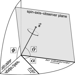
Figure 1.— Angles used to describe the observing geometry. The orbital spin axis is denoted $\vec{s}$. The contact binary is assumed located at the vertex where the angles $\theta$ (aspect, the angle between the orbital spin axis and the line-of-sight), $\alpha$ (phase, the angular distance between the Sun and the observer, as seen from the object), and $\phi$ (azimuth, the sky-plane angle between the projections of the orbital spin axis and the object-Sun vector) are measured.

Table 1Four close/contact binary systems considered.

#	$q$	($B/A,C/A$)	($b/a,c/a$)	$l$	H.E.
1	1.00	(0.66, 0.60)	(0.66, 0.60)	1.00	yes
2	0.67	(0.77, 0.69)	(0.53, 0.49)	1.00	yes
3	0.25	(0.92, 0.83)	(0.51, 0.48)	1.19	yes
4	0.13	(1.00, 0.90)	(0.51, 0.48)	1.00	no

2. High Phase Angle Lightcurves

The characteristic morphological features of contact binary lightcurves are the large range of variation, typically 0.9 mag or more, the rounded, inverted-U shaped maxima, and the sharp V shaped minima (Zappala et al., 1980; Leone et al., 1984). However, these traits appear only at phase angles close to $\alpha=0\arcdeg$. Figure 2 shows lightcurves of a symmetric contact Roche binary (system #1 from Table 1) at four different phase angles, $\alpha=1$, 30, 60, and 90$\,\arcdeg$. The surface scattering of light is modelled using a Lommel-Seeliger function, taken to represent a low albedo, lunar-type surface. The procedure used for generating the model lightcurves of Roche binaries, as well as of Jacobi triaxial ellipsoids, is described in detail in Lacerda & Jewitt (2007). The most noticeable mutations as $\alpha$ increases include:

1. the shape of the minimum changes from V-shaped first to flat and then to slightly W-shaped;

2. the transition between low and high brightness becomes sharper;

3. the positions (in rotational phase) of the minima and maxima drift to the left;

4. the overall brightness decreases, as the illuminated fraction of the surface diminishes;

5. the trough-to-peak range of variation increases.

Below, we discuss some of these points in more detail.

2.1. Lightcurve Shape and Detection Probability

As a consequence of points 1 and 2 above, the probability of detecting the total range of brightness variation from only a few measurements increases significantly with $\alpha$. This is shown in Fig. 3 where we plot the probability of measuring the extent of variation of a contact binary lightcurve for different values of $\alpha$. The Figure was generated as follows: each of the four lightcurves in Fig. 2 (corresponding to each $\alpha$) was sampled five times at random rotational phases, and the maximum range $\Delta m_{i}$ within the set of five measurements was registered. This procedure was then repeated for $i=1$ to 10000, and the cumulative distribution of ranges $\Delta m_{i}$ was plotted for each $\alpha$, starting from the maximum range. The plot shows that beyond $\alpha\sim 60\arcdeg$ most five-point samples of the lightcurve are able to identify a variation larger than 1 mag. For example, at $\alpha=60\arcdeg$ there is $\sim$80% chance of detecting a $\Delta m\geq 1\,$mag from five sparse observations of the contact binary considered.

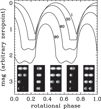
Figure 2.— Change in lightcurve morphology with increasing phase angle. Lines are labelled with the corresponding phase angles ($\alpha=1\arcdeg,30\arcdeg,60\arcdeg,$ and $90\arcdeg$). Insets show rendering of the binary used to produce the lightcurves (phase angle increasing from top to bottom) at rotational phases $\phi=0.1,0.3,0.5,0.7,$ and $0.9$.

Figure 3 was obtained assuming the most favorable observing geometry (Fig. 1): $\theta=90\arcdeg$, measured between the spin pole and the line-of-sight, and $\phi=90\arcdeg$, measured in the plane of the sky between the spin pole and the object-Sun vector. The total range of a contact binary lightcurve decreases with the aspect angle $\theta$ at about 0.03 to 0.04 mag/$\arcdeg$ (Lacerda & Jewitt, 2007); the maximum range is obtained at $\theta=90\arcdeg$. The azimuthal angle $\phi$ also influences the lightcurve range and shape. As $\phi$ moves away from 90$\arcdeg$ (the direction does not matter) the lightcurve becomes asymmetric and the range of variation is slightly decreased (Fig. 4a). Therefore, requiring a favorable geometry, i.e., angles larger than chosen minimum values $\theta>\theta_{\mathrm{m}}$ and $\phi>\phi_{\mathrm{m}}$ reduces the probability of detection of large $\Delta m$. Assuming randomly oriented spin axes, the probability of having simultaneously favorable $\theta$ and $\phi$ is given by

$$1-\frac{2}{4\,\pi}\,\Big{[}\int_{0}^{\theta_{\mathrm{m}}}\int_{0}^{2\,\pi}\sin(\theta)\,d\phi\,d\theta\,+$$

$$\int_{\theta_{\mathrm{m}}}^{\frac{\pi}{2}}\int_{-\phi_{\mathrm{m}}}^{\phi_{\mathrm{m}}}\sin(\theta)\,d\phi\,d\theta\Big{]}=\frac{\left(\pi-\phi_{\mathrm{m}}\right)}{\pi}\,\cos(\theta_{\mathrm{m}}),$$

which for minimum aspect and azimuth $\theta_{\mathrm{m}}=\phi_{\mathrm{m}}=75\arcdeg$ is $\sim 0.15$. This probability must be taken into account when estimating the intrinsic fraction of contact binary systems from a sparsely sampled survey. At any rate, since the geometry constraint (dominated by $\theta$) is present at all phase angles the conclusion that high-$\alpha$ measurements are more effective at identifying contact binary systems holds.

Figure 4b shows how the lightcurve shape depends on the relative size and separation of the binary components. Four systems were considered – their properties are detailed in Table 1. Except for system #3, meant to represent a system formed according to the model by Ćuk mentioned in §1, all systems are Roche binaries in hydrostatic equillibrium. Systems #3 and #4 produce shallower lightcurves due to their asymmetric mass ratio, and although the maxima and minima take up a large fraction of the rotational phase, the probability of measuring the total range of variation is not as high as for the more symmetric binaries #1 and #2. In conclusion, high-$\alpha$ observations will more easily detect contact binaries with similar sized components.

Currently known binary NEOs are generally asymmetric with primary to secondary size ratios of 2 to 4 (Pravec et al., 2006). Furthermore, no very close pairs or contact binaries have been directly observed [with the possible exception of 25143 Itokawa (Scheeres et al., 2007)]. The minimum orbital period is $P=11\,$hr. Whether these are intrinsic features or the result of observational bias is still unclear, but the aptness of the method presented here to find symmetric contact binaries should help throw light on the subject. The intrinsic fraction of close and contact binaries is a powerful constraint for models of NEO binary formation and destruction.

Figure 3.— Probability of measuring a magnitude range larger than $\Delta m^{\prime}$ from random sampling each lightcurve on Fig. 2 five times. An observing geometry $\theta=\phi=90\arcdeg$ has been assumed (see text and Fig. 1).

2.2. Lightcurve Phase Shift and Spin Direction

Increasing the phase angle $\alpha$ produces a shift in the rotational phase of the lightcurves (see Fig. 2). The shift happens respectively to the left or right depending on the object being illuminated from the left or right side, from the observer’s standpoint. We measure a linear rotational phase shift with a slope $\sim 1.4\times 10^{-3}$ per degree phase angle. The shift slope is similar for all four systems in Table 1. This effect must be taken into account when fitting a single rotation period to data taken at different phase angles if not to be confused with evidence for complex rotation.

As mentioned in §2.1, if the geometry is such that $\phi\neq 90\arcdeg$ then asymmetries arise in the lightcurve. The direction of the asymmetry depends on the sense of rotation of the binary. Figure 4c illustrates this effect. The asymmetry can thus be used to infer the sense of spin of the binary.

2.3. Lightcurve Range

Careful inspection of Fig. 2 shows that the lightcurve range increases with $\alpha$. This is more easily seen in Fig. 4d where lightcurve range is plotted versus phase angle (APR) for each of the four systems in Table 1. For comparison, a thin black solid line illustrates the same dependence for a triaxial Jacobi ellipsoid with axis ratios $b/a=0.60$ and $c/a=0.43$.

We find that, with the exception of the symmetric binary #1, the APRs of binary systems appear less regular than that of the ellipsoid. Binary APRs show two roughly linear regimes, steeper for lower $\alpha$ and shallower for larger $\alpha$. The slope only seems to depend on system type for small to intermediate phase angles: beyond $\alpha\sim 50$° the slopes are similar for all systems. Systems with smaller ranges at $\alpha=1$° have shallower initial APR slopes. This is similar to what was found by Zappala et al. (1990) for ellipsoids. System #1, however, has a remarkably regular APR. The slope is 0.004 mag/° up to $\alpha\sim 75$° and 0.001 mag/° beyond that value. Incidentally, the symmetric binary 90 Antiope (Merline et al., 2000; Descamps et al., 2007) has an APR slope 0.005 mag/° (Michałowski et al., 2002), very close to that of our simulated symmetric binary. The APR is shape-dominated: the APR slopes do not depend significantly on the choice of surface scattering model.

Our results seem to indicate that less regular (more asymmetric) objects have steeper APRs. Our most regular object, the symmetric binary, has the shallowest APR. A detailed analysis of the APR of contact binary systems is beyond the scope of this letter and will be treated elsewhere.

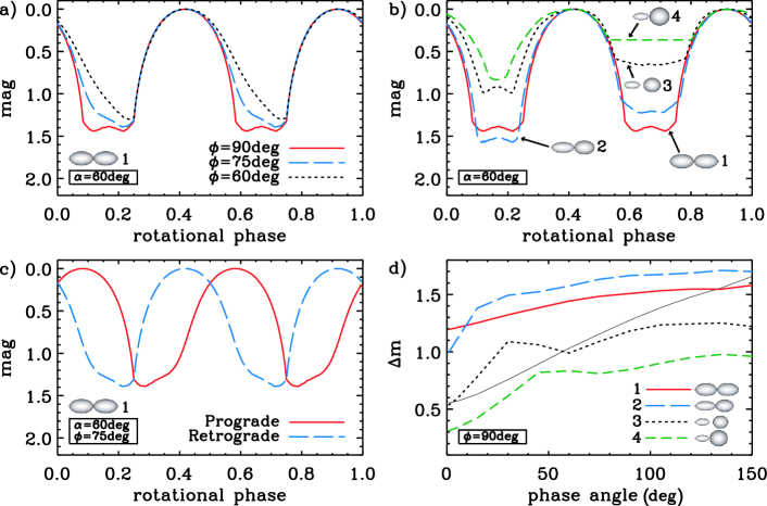
Figure 4.— a) Lightcurves of system #1 (Table 1) as a function of azimuth angle $\phi$. Geometry is $\alpha=60$°. b) Lightcurves of all four systems in Table 1 at $\alpha=60$° and $\phi=90$°. c) Asymmetric lighcurves of system #1 rotating in the prograde and retrograde directions. Asymmetry is due to observing geometry $\phi\neq 90$° and high phase angle $\alpha=60$° and shows clear dependence on the direction of rotation of the binary. d) Lightcurve range versus phase angle ($\alpha=1,5,15,30,45,60,75,90,105,120,135,$ and 150°) for each system in Table 1. Thin solid black line corresponds to a Jacobi ellipsoid with axes ratios $b/a=0.60$ and $c/a=0.43$. Observing geometry is $\phi=90\arcdeg$ (Fig. 1). All four plots assume Lommel-Seeliger lunar-type surface scattering and aspect $\theta=90$°.

3. Summary

We have presented the case for using high phase angle observations to find extreme lightcurves produced by contact binaries in the solar system. Sparse observations of contact binaries at phase angles $\alpha>60$° are extremely efficient at detecting the large range of brightness variation characteristic of these objects’ lightcurves. From Earth, this method is most relevant to observations of near-Earth objects as they attain the largest phase angles. At this point, a survey of high-$\alpha$ measurements alone should probably not be used to estimate the fraction of contact binaries in the NEO population. Deviations from hydrostatic equilibrium shape and the precise observing geometry ($\theta$ and $\phi$) affect the exact detection probability, thereby introducing uncertainty in the derived abundance. The technique is extremely efficient at detecting equator-on, relatively smooth contact binaries with symmetric components, but confirmation of the exact configuration of a system that shows large $\Delta m$ in just a few high-$\alpha$ measurements should always be sought using follow-up observations. The sparse quality of planned all-sky surveys such as Pan-STARRS implies that a full shape solution can be obtained only after several years of data have been collected. It is therefore extremely useful to develop fast techniques that allow the identification of potentially interesting targets from a Pan-STARRS-type survey (or even from dedicated surveys using sub-1m telescopes), which can be followed up on other telescopes.

References

- Bottke et al. (2006) Bottke, Jr., W. F., Vokrouhlický, D., Rubincam, D. P., & Nesvorný, D. 2006, AREPS, 34, 157
- Ćuk (2007) Ćuk, M. 2007, ApJ, 659, L57
- Ćuk & Burns (2005) Ćuk, M. & Burns, J. A. 2005, Icarus, 176, 418
- Descamps et al. (2007) Descamps, P., et al. 2007, Icarus, 187, 482
- Gehrels (1956) Gehrels, T. 1956, ApJ, 123, 331
- Lacerda & Jewitt (2007) Lacerda, P. & Jewitt, D. C. 2007, AJ, 133, 1393
- Leone et al. (1984) Leone, G., Paolicchi, P., Farinella, P., & Zappala, V. 1984, A&A, 140, 265
- Margot et al. (2002) Margot, J. L., et al. 2002, Science, 296, 1445
- Margot et al. (2003) Margot, J. L., et al. 2003, IAU Circ., 8227, 2
- Merline et al. (2000) Merline, W. J., et al. 2000, in BAAS, 1017
- Michałowski et al. (2002) Michałowski, T., et al. 2002, A&A, 396, 293
- Nolan et al. (2000) Nolan, M. C., et al. 2000, IAU Circ., 7518, 2
- Ostro et al. (1990) Ostro, S. J., et al. 1990, Science, 248, 1523
- Ostro et al. (2002) Ostro, S. J., et al. 2002, Asteroids III, 151
- Pravec & Hahn (1997) Pravec, P. & Hahn, G. 1997, Icarus, 127, 431
- Pravec et al. (2006) Pravec, P., et al. 2006, Icarus, 181, 63
- Pravec et al. (1998) Pravec, P., Wolf, M., & Sarounova, L. 1998, Icarus, 133, 79
- Scheeres (2007) Scheeres, D. J. 2007, Icarus, 189, 370
- Scheeres et al. (2007) Scheeres, D. J., et al. 2007, Icarus, 188, 425
- Ďurech & Kaasalainen (2003) Ďurech, J. & Kaasalainen, M. 2003, A&A, 404, 709
- Weidenschilling (1980) Weidenschilling, S. J. 1980, Icarus, 44, 807
- Zappala et al. (1990) Zappala, V., Cellino, A., Barucci, A. M., Fulchignoni, M., & Lupishko, D. F. 1990, A&A, 231, 548
- Zappala et al. (1980) Zappala, V., Scaltriti, F., Farinella, P., & Paolicchi, P. 1980, Moon and Planets, 22, 153