Potts-Percolation-Gauss Model of a Solid
Abstract
We study a statistical mechanics model of a solid. Neighboring atoms are connected by Hookian springs . If the energy is larger than a threshold the spring is more likely to fail, while if the energy is lower than the threshold the spring is more likely to be alive. The phase diagram and thermodynamic quantities, such as free energy, numbers of bonds and clusters, and their fluctuations, are determined using renormalization-group and Monte-Carlo techniques.
pacs:
05.10.Ln,05.10.Cc,62.20.-xI Introduction
The mechanical properties of solids, such as the mechanical failure, are topics of considerable interest.Arcangelis ; Beale ; Bolander ; Buxton ; Yanay In this paper we analyze an equilibrium statistical mechanics modelBlumberg of a solid. In previous calculationsKaufman96 we went beyond the ideal Hooke law for springs by using the realistic anharmonic energy versus atomic distance developed and tested extensively by Ferrante and his collaborators.Rose We found that the phase diagram exhibits universal features when the temperature and the stress are appropriately scaled. Those calculations were mean-field in character as we assumed that all springs have the same strain. In this paper we evaluate the role of thermal fluctuations by using renormalization-group and Monte-Carlo simulations. The model is defined in Section II. We view the solid as a collection of harmonic springs. If the energy of such a spring is larger than a threshold, the spring is likely to fail.Hassold Assuming that the relaxation times are short compared to the measurement time, we use equilibrium statistical mechanics to compute the various thermodynamic quantities. When the elastic energy is not too large, the partition function for the harmonic ”springs” defined on percolation clusters can be mapped into a Potts model. Potts ; Wu This model is quite similar to the annealed Ising model on percolation cluster.Kaufman94 ; Scholten In Section III we present numerical results based on the renormalization-group Migdal-Kadanoff scheme which, as first shown by BerkerBerker , provides exact solutions of statistical models on hierarchical lattices Kaufman81 ; Kaufman84 ; Erbas and on small world nets.Hinczewski ; Rozenfeld Monte-Carlo simulations are presented in Section IV. Our concluding remarks are found in Section V.
II Model
The energy of a ”spring” is given by the Hooke law:
| (1) |
where is the displacement vector from the equilibrium position of atom , measured in units of the lattice constant , is the cohesive energy, and is elastic constant. If the energy of the spring is larger than the threshold energy the ”spring” is more likely to fail than to be alive. is the probability that the ”spring” is alive and the probability that the ”spring” breaks. We assume its dependence on energy to be given by the Boltzmann weight
| (2) |
where: and . We allow for correlations between failing events by using the PottsPotts number of states , which plays the role of a fugacity controlling the number of clustersKaufman84b ; Hu : if there is a tendency of forming many small clusters while if there is a tendency to form a few large clusters. If springs fail independently of one another, i.e. random percolation problemFortuin . The partition function is obtained by summing over all possible configurations of bonds arranged on the lattice
| (3) |
is the number of clusters, including single site clusters, and is number of live ”springs”. The restricted partition function associated with the elastic energy for a given configuration of bonds (live ”springs”) is
| (4) |
| (5) |
In Eq. (5) the sum is over all live ”springs”.
By using the Kasteleyn-Fortuin expansionFortuin for Potts model we can rewrite the partition function as
| (6) |
The Hamiltonian is
| (7) |
where is a Potts spin taking values. This mapping is a Gaussian approximation valid when, on the right hand side of Eq. 7, the elastic energy is small compared to the first energy contribution. The coupling constants and are related to the original parameters, and , as follows:
| (8) | |||||
| (9) |
The free energy per bond is: . The derivatives of the free energy with respect to the parameters , , and provide respectively the number of live ”springs” , the elastic energy and the number of clusters , each normalized by the total number of lattice bonds:
| (10) | |||||
| (11) | |||||
| (12) |
The derivatives of those densities, , , and , with respect to the model parameters provide in turn the fluctuations (variances) of those quantities:
| (13) | |||||
| (14) | |||||
| (15) |
III Renormalization Group
The Migdal-Kadanoff recursion equationsMigdal ; Kadanoff for dimensions are: , where . We assume each atom coordinate varies in the interval (-1/2, 1/2), where the equilibrium lattice constant is 1. After also using the Gaussian approximation (small elastic energy) we get:
| (16) | |||||
| (17) |
where and
| (18) |
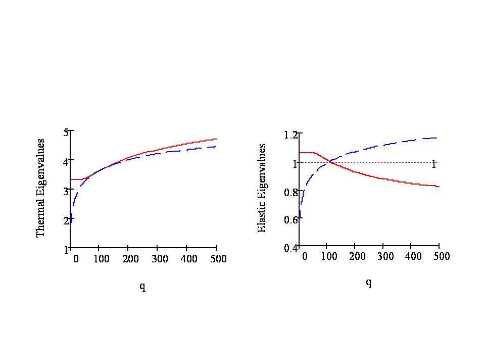
The recursion equations (16)-(17) represent the Gaussian approximation of the exact solutions for hierarchical lattices. Since this scheme is realizable, the convexity of the free energy is preservedKaufman83 , and thus reasonable expectations, such as positivity of energy fluctuations, are fulfilled. The renormalization group flows are governed by the following fixed points at (pure Potts model): i. (non-percolating live ”springs”), ii. (percolating network of live ”springs”), iii. (Potts critical point). A stability analysis at the Potts critical point, (, ) yields the two eigenvalues: i. the thermal eigenvalue (for the direction along the axis) is always larger than 1, meaning the is a relevant field; ii. The other eigenvalue is associated with the flow along the line away from the pure model (). For , for all . This means that there is a line of points in the flowing into, and thus is in the same universality class as, the pure Potts critical point (. For on the other hand, for , but for . There exists another fixed point at which has both eigenvalues larger than unity for , and becomes stable in one direction for . Thus in , for large enough , the elastic constant becomes a relevant field changing the universality class of the model from the pure Potts criticality to a new one, Potts-elastic. However, in view of the Gaussian approximation used to derive the recursion equations, we view this as only an indication of a possible new universalty class that warrants further study.
The phase diagram for any given , in the plane shows two phases: I. solid with a percolating network of live ”springs”, II. crumbling solid with mostly ”failed” springs. The two phases are separated by a critical line in the universality class of the -state Potts model (for for all , for for ).
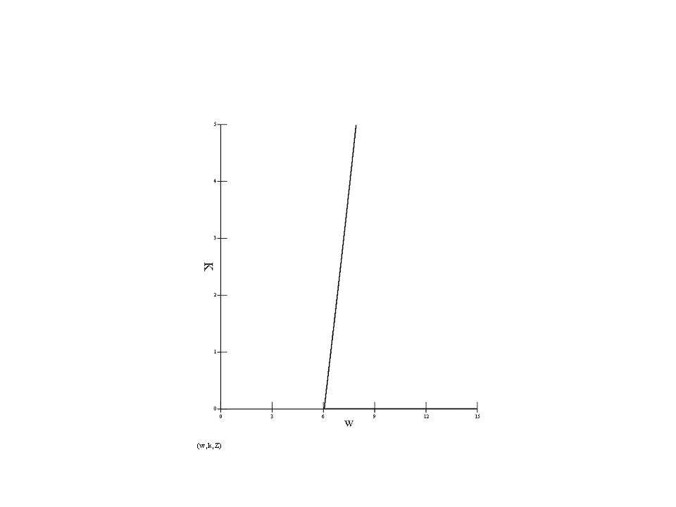
Note that when increasing the elastic constant , one needs a higher to establish the solid phase. This is due to the fact that increasing the elastic energy increases the probability for the ”spring” to fail.
The free energy , where is the number of lattice edges, is:
| (19) |
where
| (20) |
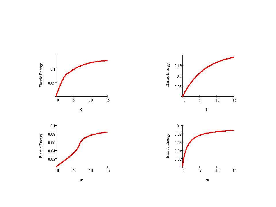
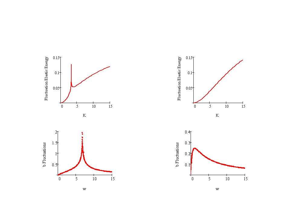
and . Using the free energy we can compute the number of live ”springs” , the number of clusters , the elastic energy , and their fluctuations (variances). Each of those quantities is scaled by the total number of lattice edges . In Figure 3 we show the elastic energy variation with K and w for two different q values. As expected the elastic energy increases monotonically with K and w starting at zero at K = 0 and at w = 0.
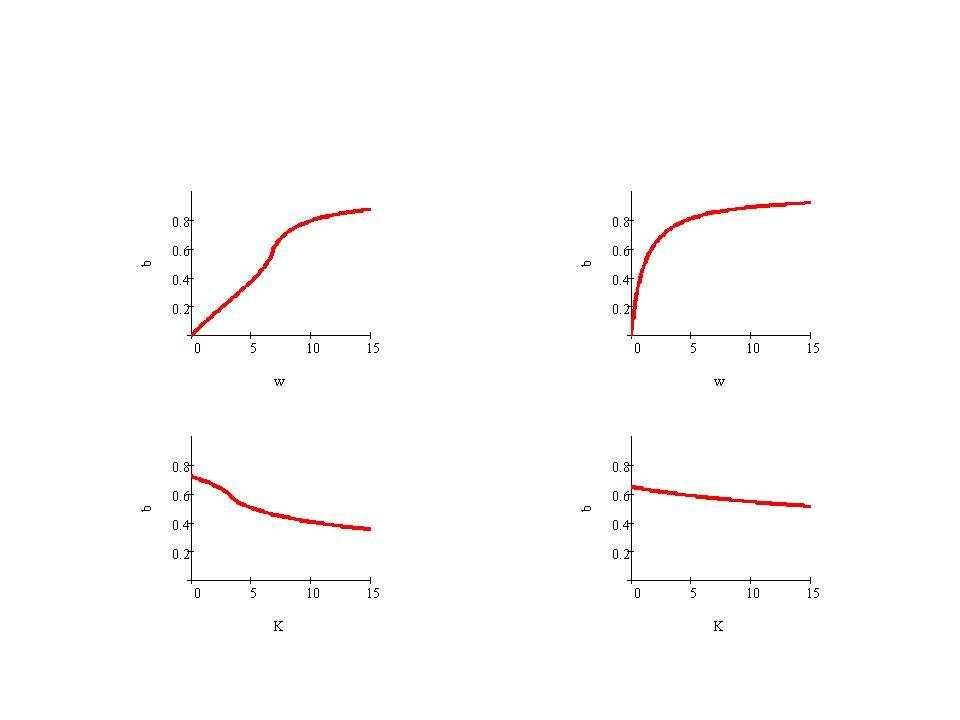
The number of live ”springs” increases with w and decreases with K, as shown in Figure 4.
We also estimate the squared mean elongation (in units of lattice constant ) of live ”sprins” by using the number of live springs, , and the elastic energy:
| (21) |
One can use the classical Lindemann model of meltingLindemann , , to estimate the melting temperature of our model solid.
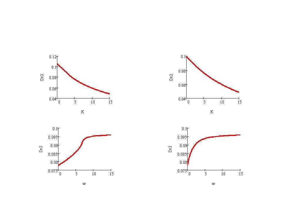
In the limit , the number of clusters is equal to the number of sites. Hence approaches the inverse of the coordination number, which for the diamond hierarchical lattice, correponding to the Migdal-Kadanoff scheme for , isKaufman84 : , consistent with Figure 6.
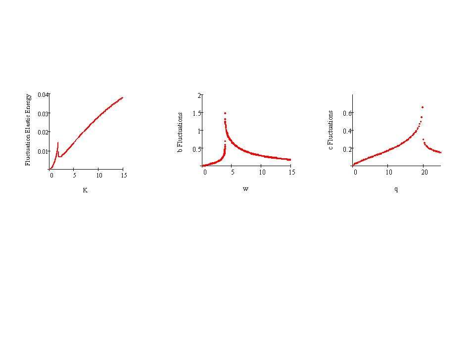
In Figure 7 we show the elastic energy fluctuations and the number of live ”springs” fluctuations as functions of and , for and = 1 respectively. Since the exponent is positive for and negative for , a divergence is apparent in the critical point , .
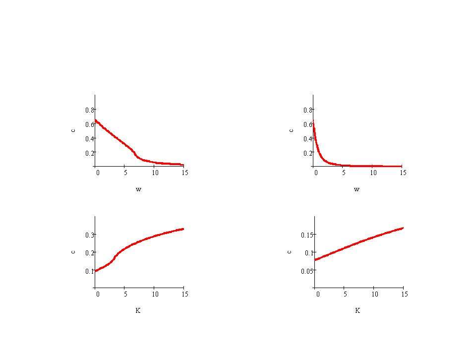
The number of clusters increases monotonically with the conjugated fugacity , starting at = 0 at = 0, as shown in Figure 8. The fluctuations in c exhibit a divergence at the critical point = 10, = 2, = 7.3 where the critical exponent is positive.
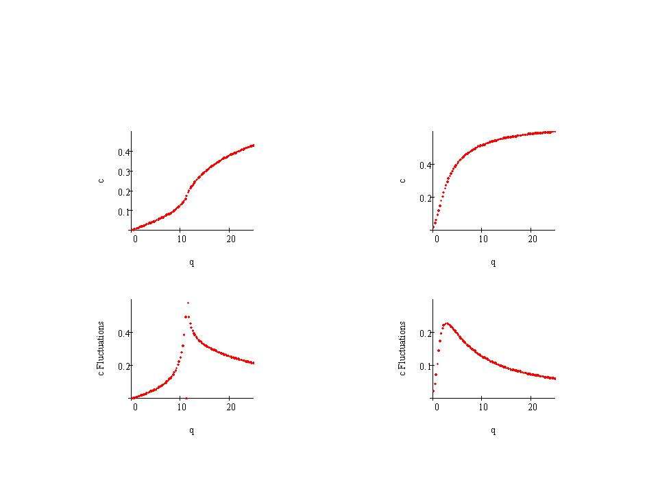
In Figure 9 we show fluctuations in elastic energy, in number of bonds, and number of clusters against , , and respectively, for and . One can notice the lack of symmetry in the divergence which is a characteristic of 3 criticalityKaufman84a ; Chase . By contrast in the divergences are symmetric (see Figure 7). This is related to the duality transformation Kaufman84a ; Kaufman84b . The critical point exponent at , , is .
IV Monte Carlo Simulations
In this section, we use for Monte Carlo simulation the following Hamiltonian taken from Eq. (7)
| (22) |
where and are renormalized parameters. Of course, one has and .
In the case of two dimensions , we consider a square lattice of size where . Each lattice site is occupied by a state Potts spin. We use periodic boundary conditions. Our purpose here is to locate the phase transition point and establish the phase diagram. To this end, a simple heat-bath Metropolis algorithm is sufficient.Binder The determination of the order of the phase transition and the calculation of the critical exponents in the second-order phase transition region need more sophisticated Monte Carlo methods such as histogram techniques.Ferren These are left for a future study.
The simulation is carried out as follows. For each set of , we equilibrate the system at a given temperature during Monte Carlo sweeps (MCS) per spin before averaging physical quantities over the next MCS. In each sweep, both the spin value and the spin position are updated according to the Metropolis criterion. The calculated physical quantities are the internal energy per spin , the specific heat per spin, the Potts order parameter and the susceptibility per spin . For a -state Potts model, is defined as
where (, being the number of sites having .
Let us show first in Fig. 10 and Fig. 11 the energy, the specific heat, the order parameter and the susceptibility in the case where , and .
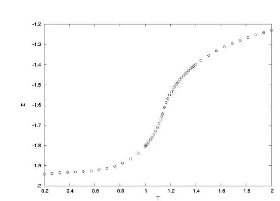
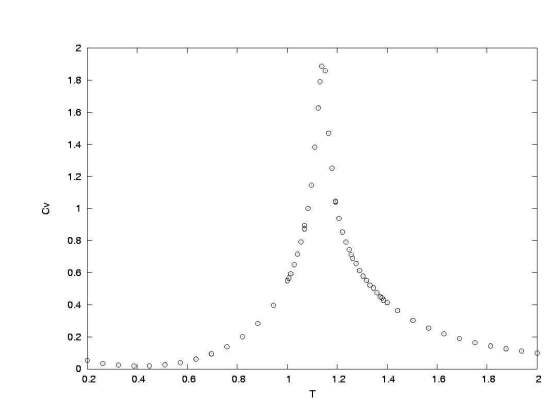
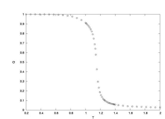
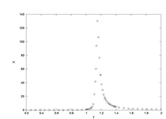
These figures show a phase transition at . Note that the size effects for , 60, 80 and 100 are not significant and are included in the error estimation. Simulations have been carried out also for the following sets , and . The results show that the transition temperature does not change significantly with this range of . depends only on the main term.
To compare with the results from the renormalization group calculation of the previous section, we have to use , and Eqs. (8-9) to convert and into and . One has
| (23) | |||||
| (24) |
where .
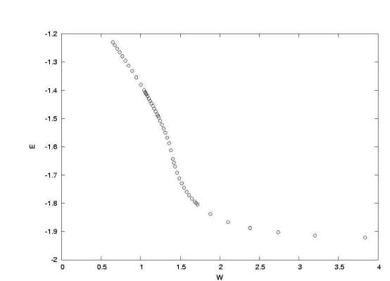
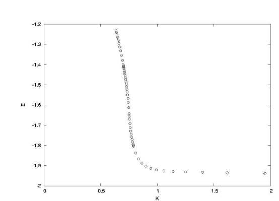
Figure 12 shows the internal energy as functions of and for and . The transition is found at and . We observe that only varies with , not as expected from Eqs. (23)-(24). We have and for and 1, respectively.
V Conclusions
We have studied a model of a solid made of springs that are live and harmonic or failed. The springs can fail with a probability that increases with the energy. Our renormalization-group analysis suggests that elastic perturbations on the Potts-percolation model are irrelevant for all in two dimensions, and for small enough in three dimensions. The renormalization-group predictions must be viewed as only indicative, in view of the following known limitations. The simple Migdal-Kadanoff renormalization group fails to predict correctly the first-order transitions for , , and for , . Furthermore our recursion equations are valid for small elastic energy. Monte Carlo simulations are needed to further our understanding of the model. Monte Carlo results in show that the phase transition does not depend on both on the value of the transition temperature and on the transition order. This is physically in agreement with the fact that in two dimensions the melting does not take place at finite temperature. At least in , one can say that the phase transition is solely due to the first term of the Hamiltonian (22). We note in passing that in the Ising case, the question of whether the elastic interaction affects or not the Ising universality class has been investigated.Bergmann ; Fisher68 No definite conclusions have been reached.Diep ; Landau It would be therefore interesting in the future to perform Monte Carlo simulations for and for large to investigate the effect of elastic interaction on the criticality and on cross-over from second to first-order.
References
- (1) L. De Arcangelis, A. Hansen, H. J. Hermann, S. Roux, Phys. Rev. B 40, 877 (1989).
- (2) P. D. Beale, D. J. Srolovitz, Phys. Rev. B 37, 5500 (1988).
- (3) J. E. Bolander, N. Sukumar, Phys. Rev. B 71, 094106 (2005).
- (4) G. A. Buxton, R. Verberg, D. Jasnow, A. C. Balazs, Phys. Rev. E 71, 056707 (2005).
- (5) Y. Yanay, A. Goldsmith, M. Siman, R. Englman, Z. Jaeger, J. Appl.Phys. 101, 104911 (2007).
- (6) R. L. Blumberg Selinger, Z. G. Wang, W. M. Gelbart, A. Ben-Shaul, Phys. Rev. A 43, 4396 (1991).
- (7) M. Kaufman, J. Ferrante, NASA Tech. Memo. 107112 (1996).
- (8) J. H. Rose, J. Ferrante, J. R. Smith, Phys. Rev. Lett. 47 , 675 (1981); J. H. Rose, J. R. Smith, F. Guinea, J. Ferrante, Phys. Rev. B 29, 2963 (1984); J. Ferrante, J. R. Smith, Phys. Rev. B 31, 3427 (1985).
- (9) G. N. Hassold and D. J. Srolovitz, Phys. Rev. B 39, 9273 (1989).
- (10) R. B. Potts, Proc. Camb. Phil. Soc. 48, 106 (1952).
- (11) F. Y. Wu, Rev. Mod. Phys. 54, 235-268 (1982).
- (12) M. Kaufman and J. E. Touma, Phys. Rev. B 49, 9583 (1994).
- (13) P. D. Scholten and M. Kaufman, Phys. Rev. B 56, 59 (1997).
- (14) A. N. Berker and S. Ostlund, J. Phys. C 12, 4961-4975 (1979).
- (15) M. Kaufman, R.B. Griffiths, Phys. Rev. B 24, 496 (1981).
- (16) M. Kaufman, R.B. Griffiths, Phys. Rev. B 30, 244 (1984).
- (17) A. Erbas, A. Tuncer, B. Yucesoy, A. N. Berker, Phys Rev E 72, 026129 (2005).
- (18) M. Hinczewski, A. N. Berker, Phys. Rev. E 73, 066126 (2006).
- (19) H. D. Rozenfeld, D. ben-Avraham, Phys Rev E 75, 061102(2007).
- (20) M. Kaufman, D. Andelman, Phys. Rev. B 29, 4010-4016 (1984).
- (21) C.-K. Hu and C. N. Chen, Phys. Rev. B 38, 2765 (1988).
- (22) C. M. Fortuin, P. W. Kasteleyn, J. Phys. Soc. Jpn. Supplm. 26, 11 (1969).
- (23) A. A. Migdal, JETP (SovPhys)42, 743 (1976).
- (24) L. P. Kadanoff, Ann. Phys.(NY) 100, 359 (1976).
- (25) M. Kaufman, R.B. Griffiths, Phys. Rev. B 28, 3864 (1983).
- (26) F. A. Lindemann, Z. Phys 11, 609 (1910).
- (27) M. Kaufman, Phys. Rev. B 30, 413(1984).
- (28) S. I. Chase, M. Kaufman, Phys. Rev. B 33, 239-244 (1986).
- (29) K. Binder and D. W. Heermann, Monte Carlo Simulation in Statistical Physics, Springer (2002).
- (30) A. M. Ferrenberg and R. H. Swendsen, Phys. Rev. Lett. 61, 2635(1988); Phys. Rev. B 44, 5081(1991).
- (31) D. J. Bergmann and B. I. Halperin, Phys. Rev. B 13, 2145 (1976) and references therein.
- (32) M. E. Fisher, Phys. Rev. 176, 257 (1968).
- (33) E. H. Boubcheur and H. T. Diep, J. Appl. Phys. 85, 6085 (1999); E. H. Boubcheur , P. Massimino, H. T. Diep, J. of Magn. and Magn. Mater. 223, 163-168 (2001) and references therein.
- (34) Xiaoliang Zhu, D. P. Landau, and N. S. Branco, Phys. Rev. B 73, 064115 (2006).