Structural parameters for globular clusters in NGC 5128. III.
ACS surface-brightness profiles and model fits

Abstract

We present internal surface-brightness profiles, based on HST/ACS imaging in the $F606W$ bandpass, for 131 globular cluster (GC) candidates with luminosities $L\simeq 10^{4}$–$3\times 10^{6}\,L_{\odot}$ in the giant elliptical galaxy NGC 5128. Several structural models are fit to the profile of each cluster and combined with mass-to-light ratios from population-synthesis models, to derive a catalogue of fundamental structural and dynamical parameters parallel in form to the catalogues recently produced by McLaughlin & van der Marel and by Barmby et al. for GCs and massive young star clusters in Local Group galaxies. As part of this, we provide corrected and extended parameter estimates for another 18 clusters in NGC 5128, which we observed previously. We show that, like GCs in the Milky Way and some of its satellites, the majority of globulars in NGC 5128 are well fit by isotropic Wilson models, which have intrinsically more distended envelope structures than the standard King lowered isothermal spheres. We use our models to predict internal velocity dispersions for every cluster in our sample. These predictions agree well in general with the observed dispersions in a small number of clusters for which spectroscopic data are available. In a subsequent paper, we use these results to investigate scaling relations for GCs in NGC 5128.

1 Introduction

The spatial structures and internal stellar kinematics of old globular clusters (GCs) contain information on both their initial conditions and their dynamical evolution over a Hubble time. An efficient way of extracting this information is to fit detailed models to the surface-brightness profiles and (where available) velocity-dispersion data of individual clusters, and then to look for possible correlations between the physical properties of large numbers of GCs. This has been done for most of the $\simeq\!150$ globulars in the Milky Way, yielding comprehensive catalogues of their structural and dynamical parameters (Djorgovski, 1993; Pryor & Meylan, 1993; Harris, 1996; McLaughlin & van der Marel, 2005). Much of this work has traditionally started from the assumption that individual globulars are well described by the classic King (1966) models of single-mass, isotropic, modified isothermal spheres, although recently alternative models have also been employed (McLaughlin & van der Marel, 2005).

Explorations of numerous scaling relations and interdependences between the properties of Galactic GCs (e.g., Djorgovski & Meylan, 1994) have led to the definition of a fundamental plane for globulars that is analogous to but physically distinct from that for early-type galaxies and bulges (Djorgovski, 1995; Burstein et al., 1997; McLaughlin, 2000). Understanding the GC fundamental plane in full detail is still not a completely solved problem, but important advances have been made in recent years as it has become possible to measure the internal properties of GCs in many other galaxies. High-resolution Hubble Space Telescope (HST) imaging has been used to fit King (1966) and other models to the surface-brightness profiles of scores of globulars in the Large and Small Magellanic Clouds and the Fornax dwarf spheroidal (Mackey & Gilmore, 2003a, b, c; McLaughlin & van der Marel, 2005), M31 (e.g., Barmby, Holland, & Huchra, 2002; Barmby et al., 2007), M33 (Larsen et al., 2002), and the giant elliptical galaxy NGC 5128 = Centaurus A (Holland, Côté, & Hesser 1999; Harris et al. 2002). Internal velocity dispersions and dynamical mass estimates are also available for smaller but growing numbers of GCs in these systems (Djorgovski et al., 1997; Dubath & Grillmair, 1997; Larsen et al., 2002; Martini & Ho, 2004; Rejkuba et al., 2007).

Here we add to this database with structural measurements of 131 GCs in NGC 5128. This galaxy is an attractive target for such studies in part because of its large GC population, estimated by Harris et al. (2006) at ${\cal N}_{\rm GC}\simeq 1500$. It thus contains many objects at the high end of the star-cluster mass range ($10^{6}$–$10^{7}\ M_{\odot}$), which is largely unprobed in the ten-times smaller GC system of the Milky Way but where it is increasingly suggested that the cluster population may encompass a variety of objects including classic globulars, the compact nuclei of dwarf elliptical galaxies, and the new class of ultra-compact dwarf galaxies (Hilker et al., 1999; Drinkwater et al., 2000; Haşegan et al., 2005). In addition, the proximity of NGC 5128 ($D=3.8$ Mpc; see below) makes it possible to resolve the core radii as well as just the half-light radii of GCs over nearly their full mass range ($M\ga 10^{4}\ M_{\odot}$), and thus to fit them rigorously with detailed structural models.

This paper is the third in a series of four dealing with HST observations of GCs in NGC 5128. In Harris et al. (2002, $\equiv$ Paper I) the Space Telescope Imaging Spectrograph (STIS) and Wide Field Planetary Camera 2 (WFPC2) aboard HST were used to measure surface-brightness profiles for 27 very bright GCs in NGC 5128. King (1966) models were fitted to these profiles to derive a structural fundamental plane that could be compared directly to that of the Milky Way globulars. In Harris et al. (2006, $\equiv$ Paper II) we published the first results from a new HST-based survey of GCs in NGC 5128, using the Advanced Camera for Surveys (ACS) in its Wide Field Channel (WFC) to image a total of 131 GC candidates at a resolution of 0$\aas@@fstack{\prime\prime}$05 (linear resolution $\simeq\!0.9$ parsec). Paper II gives the full description of the cluster sample along with some rough overall characteristics of the ensemble of objects. In the present paper, we derive surface brightness profiles for all of these clusters and fit each of them with a number of different structural models. The final paper in this series (McLaughlin et al., 2007, $\equiv$ Paper IV) uses these results to examine a number of structural correlations for GCs in NGC 5128, which are then compared to the globulars in the Milky Way and to various other types of massive clusters. In related work, Barmby et al. (2007) present the results of a similar ACS study of GCs in M31 and compare the fundamental planes of old GCs in that galaxy, the Milky Way, NGC 5128, the Large and Small Magellanic Clouds, and the Fornax dwarf spheroidal.

In the next Section we describe the steps we have taken to derive surface brightness profiles for the GC candidates from Paper II, to characterise the point-spread function (PSF) that blurs the very central regions ($R\la 2$–3 pc) of these profiles, to transform the surface-brightness data from their native HST filter to the standard $V$ bandpass, and to estimate metallicities for the clusters from separate, ground-based Washington photometry.

In §3, we apply publicly available population-synthesis models to estimate individual $V$-band mass-to-light ratios for the clusters, given their metallicities and assuming various (old) ages. Following this, we summarise the main properties of each of three structural models (those of King 1966, Wilson 1975, and Sérsic 1968) that we have convolved with the ACS/WFC PSF and fit to every observed surface-brightness profile.

Section 4 gives the results of these fits and uses them to infer a wide range of structural and dynamical parameters, including total cluster luminosities and masses, effective and core radii and stellar densities, concentration indices, relaxation times, total binding energies, predicted central velocity dispersions, and $\kappa$-space parameters for the fundamental plane (Bender, Burstein, & Faber, 1992). We present these in tables that are available in machine-readable format either online or upon request from the first author. Note that our measurements of GC luminosities and intrinsic sizes in particular supersede the recent estimates of van den Bergh (2007), who based his numbers on a less detailed analysis of some very basic cluster characteristics given in Paper II.

In §4 we also address the question of whether the standard King (1966) model specifically gives the best possible fit to GC surface-brightness profiles in NGC 5128. We then extend the range of physical parameters calculated for the smaller sample of clusters previously fitted with King models in Paper I, and we provide important corrections to some of the more basic parameters (in particular, the intrinsic central surface brightnesses) already published in that earlier work. The results of this re-analysis are tabulated in Appendix A.

In §5 we combine our structural modeling and population-synthesis mass-to-light ratios to predict line-of-sight velocity dispersions within a series of circular apertures with physical radii suited to realistic observational set-ups. We compare these predictions with spectroscopic data from Martini & Ho (2004) and Rejkuba et al. (2007) for some of our current cluster sample. Finally, §6 summarises the paper.

Our modeling analysis in this paper is in all respects very similar to that undertaken by McLaughlin & van der Marel (2005) for a sample of 103 old GCs and 50 young massive clusters drawn from the Milky Way, the Large and Small Magellanic Clouds, and the Fornax dwarf spheroidal. The catalogues of structural and dynamical properties that we produce here for GCs in NGC 5128 are likewise very close in form and content to those in McLaughlin & van der Marel. We have recently completed the same type of modeling and produced parallel catalogues for a further 93 GCs in M31 (Barmby et al., 2007). As we mentioned above, Barmby et al. combine results to compare the fundamental planes of the old GCs in all six galaxies. In Paper IV (McLaughlin et al., 2007) we directly compare GC structural correlations only between the Milky Way and NGC 5128, but we also examine how they relate to other kinds of massive star clusters.

In all of what follows, we adopt a distance of 3.8 Mpc to NGC 5128. This value is representative of recent measurements based on the tip of the red-giant branch [$(m-M)_{0}=27.98\pm 0.15$], the planetary nebulae luminosity function [$(m-M)_{0}=27.97\pm 0.14$], surface-brightness fluctuations [$(m-M)_{0}=27.78\pm 0.10$], Mira variables [$(m-M)_{0}=27.96\pm 0.11$], and Cepheids [$(m-M)_{0}=27.67\pm 0.20$]; see Harris, Harris, & Poole (1999), Rejkuba (2004), and Ferrarese et al. (2007). The nominal average of these five, reasonably high-precision distances is $(m-M)_{0}=27.88\pm 0.06$, or $3.76\pm 0.11$ Mpc. All these methods have undergone recent calibration revisions of various kinds (cf. Ferrarese et al., 2007) but the net results have been to shift the mean up or down by amounts at the level of only $0.1$ mag. At a distance of 3.8 Mpc, 1 arcsecond is subtended by 18.4 parsec. One ACS/WFC pixel (0$\aas@@fstack{\prime\prime}$05) then corresponds to 0.92 pc.

2 Data

The GC sample from Paper II consists of 62 previously known clusters in NGC 5128, and 69 newly discovered candidates. All these objects fall in 12 target fields imaged in the $F606W$ (“wide $V$”) band on the ACS/WFC. We observed 16 clusters twice, since they appeared in two overlapping target fields. These are listed in Table 1. We measured two independent surface-brightness profiles for each of them, so that in all we have 147 profiles for 131 distinct objects. In §4.3 we use these duplications to assess whether variations in the PSF over the ACS field of view might have systematically affected our results.

Of the 27 GCs observed with STIS or WFPC2 in Paper I, 9 were re-observed with the ACS/WFC for Paper II and this paper; these are C007, C025, C029, C032, C037, C104, C105, G221, and G293. Our analysis of them here supersedes that in Paper I. We eventually fold the other 18 STIS/WFPC2 clusters into the sample for correlations work in Paper IV, although with structural parameters updated as discussed in §4.6 and Appendix A below.

We repeatedly convert between luminosities and masses by assigning individual $V$-band mass-to-light ratios to all GCs in our total sample. As we describe in more detail below (§2.3 and §3.1), to do this we first estimate a metallicity for each cluster from its $(C-T_{1})$ colour in the Washington filter system, using a relation calibrated against genuinely old GCs. Then, we input this and an assumed old age (normally 13 Gyr) to a standard population-synthesis code. Spectroscopy indicates that most of the GCs in NGC 5128 are indeed old, but a younger (few Gyr) population cannot be ruled out at this stage. If some of the objects in our sample are young, then the mass-to-light ratio we assign to them would be slightly high, and all physical parameters deriving from it would be slightly biased. One way to guard somewhat against this is not to include exceedingly blue objects with unrealistically low inferred metallicities (see Table 5) in detailed studies of parameter correlations and the like.

Table 1: NGC 5128 clusters measured independently on two fields${}^{~{}a}$

Cluster	Fields	Cluster	Fields
(1)	(2)	(1)	(2)
AAT118198	C018, C019	C171	C007, C025
AAT120976	C007, C025	C173	C007, C025
C007	C007, C025	C176	C007, C025
C018	C018, C019	F1GC20	C007, C025
C025	C007, C025	G221	C007, C025
C104	C007, C025	G293	C007, C025
C156${}^{~{}b}$	C018, C019	PFF021	C003, C030
C158	C018, C019	WHH22	C018, C019

^a Boldface in column (2) denotes the field in which the cluster in column (1) is closest to the centre of the chip. Model fits to the intensity profiles from these images are the ones used in the correlation analyses of Paper IV.

^b Possible star; see Table 2.

2.1 Surface-brightness profiles

We have used the STSDAS ELLIPSE task to obtain $F606W$ surface-brightness profiles for all cluster candidates from Paper II. As part of the same HST program (GO-10260), we also obtained ACS images for a series of clusters in M31. These data were reduced and modeled simultaneously with the present sample and are discussed in Barmby et al. (2007). Full details of the surface-photometry procedures are given in that paper. Here we note that we forced the isophote ellpticity in ELLIPSE to be identically 0 at all radii. We thus always have circularly symmetric $I_{F606}(R)$ profiles, which we then fit with spherical structural models. In Paper II, we showed that the actual ellipticities of the clusters are generally quite small, averaging $\langle\epsilon\rangle=0.08$ over our whole sample. The assumption $\epsilon\equiv 0$ for the purposes of modeling is therefore not a significant limitation.

The raw output from ELLIPSE is in terms of counts per second per pixel, which we convert to ${\rm cts/s}$ per square arcsecond by multiplying by $400=(1\,{\rm px}/0\aas@@fstack{\prime\prime}05)^{2}$. Normally, these counts would then be transformed to $F606W$ surface brightnesses, calibrated on the VEGAMAG system according to (ACS Handbook)

$$\mu_{F606}/{\rm mag\ arcsec^{-2}}=26.398-2.5\,\log({\rm cts/s}/\sq\arcsec)\ .$$ (1)

However, we quickly found that the average, global sky background that was automatically subtracted from each ACS image during the multi-drizzling in the data reduction pipeline often underestimated and sometimes overestimated the local background level around individual clusters. The latter case in particular led to the occurrence of pixels with unphysical negative counts. We thus had to work immediately in terms of linear intensity (which we chose to express right away as $L_{\odot}\ {\rm pc}^{-2}$) rather than going through the usual logarithmic $\mu_{F606}$ and then converting to linear quantities later. For the solar magnitude we adopt $M_{\odot,F606}=4.64$, and combining this with equation (1) gives

$$I_{F606}/L_{\odot}\,{\rm pc}^{-2}\simeq 0.8427\times({\rm cts/s}/\sq\arcsec)\ .$$ (2)

To begin with, we obtained $I_{F606}(R)$ profiles out to $R>10\arcsec$ (more than 180 pc) for all clusters. This limit exceeds the expected tidal radius for most of them, but such a large field of view enables us to correct for the inaccurate average sky subtraction in the multi-drizzling, by fitting the profiles with PSF-convolved structural models that include a constant background term (allowed to be negative). We did have to exclude a number of isophotes from most of the intensity profiles during this fitting, however.

First, at very large radii the signal from most clusters is clearly swamped by noise, and thus we restricted all fitting to radii $R<150$ WFC pixels, corresponding to $R<7\aas@@fstack{\prime\prime}5\simeq 140$ pc.

Second, the central pixels in some of the brighter clusters were saturated. We adopted a saturation limit of 70 cts/s/px and did not fit to any isophotal intensities brighter than this. This corresponds to a “good” data range of about $I_{F606}\leq 2.36\times 10^{4}\ L_{\odot}\,{\rm pc}^{-2}$, or $\mu_{F606}\geq 15.28$ mag arcsec^-2.

Third, at intermediate clustercentric radii there are some individual isophotes with ELLIPSE intensities that deviate strongly from those of immediately neighboring isophotes. To prevent such “blips” from skewing the model fits, we first ran the ELLIPSE output through a boxcar filter to make a smoothed cluster profile, and identified points deviating from this by more than twice their own (internal) uncertainty. Such points were not included in the error-weighted model fitting of §4.

Fourth, the ELLIPSE estimates of isophotal intensities at clustercentric radii $R<2\ {\rm px}=0\aas@@fstack{\prime\prime}1$ are all derived from the data in the same innermost 13 pixels; but the task nevertheless outputs brightnesses for 15 radii inside 2 px. Clearly not all of these are statistically independent. In order to avoid having such correlations (and excessive weighting of the central regions of the cluster) bias our fits, we decided to include only the ELLIPSE intensities reported for the innermost unsaturated isophotal radius, $\equiv R_{\rm min}$ (which was always at least 0.5 px), and then for $(R_{\rm min}+0.5\ {\rm px})$, $(R_{\rm min}+1.0\ {\rm px})$, $(R_{\rm min}+2.0\ {\rm px})$, and all $R>2.5\ {\rm px}=0\aas@@fstack{\prime\prime}125$.

Table 2: Irregularities in some NGC 5128 cluster profiles

Cluster	Comments
AAT111563	Bright star nearby. Fits restricted to $R<5\aas@@fstack{\prime\prime}5\simeq 107$ pc.
AAT113992	Profile dips at $R=1\aas@@fstack{\prime\prime}5$ (30px), near image edge. Fits restricted to $R<1\arcsec\simeq 20$ pc.
AAT118198	Diffraction spike from nearby star. Fits restricted to $R<2\arcsec$.
C104 ON C025	Two nearby stars. Fits restricted to $R<5\arcsec\simeq 97$ pc.
C118	Bright object nearby. Region $0\aas@@fstack{\prime\prime}55<R<1\arcsec$ masked out of fits.
C134	Bright star nearby. Fits restricted to $R\la 3\arcsec$.
C137	Bright object nearby. Region $1\aas@@fstack{\prime\prime}2<R<2\aas@@fstack{\prime\prime}2$ masked out of fits.
C154	Cluster C153 at $R\approx 2\aas@@fstack{\prime\prime}5$. Model fits restricted to $R<1\arcsec\simeq 20$ pc.
C162	Profile dips slightly around $R\simeq 2\aas@@fstack{\prime\prime}5$, but fits not biased. No restrictions.
C168	Next to very bright star. Fits restricted to $R<1\arcsec$, which likely misses some cluster.
	Object excluded from sample for correlation analyses in Paper IV.
C171	Stars at $R=3\aas@@fstack{\prime\prime}5$ and $R=6\aas@@fstack{\prime\prime}6$. Fits restricted to $R<6\aas@@fstack{\prime\prime}6\simeq 130$ pc.
C174	Star at $R=1\aas@@fstack{\prime\prime}6$. Fits restricted to $R<1\arcsec\simeq 20$ pc.
F1GC34	Bright object at $R=2\aas@@fstack{\prime\prime}5$, and F1GC14 at $R=3\aas@@fstack{\prime\prime}3$. Fits restricted to $R<1\arcsec$.
	Object excluded from sample for correlation analyses in Paper IV.
F2GC14	In middle of image artifact (bright star ghost?). Fits restricted to $R<0\aas@@fstack{\prime\prime}7\simeq 13.5$ pc.
	Object excluded from sample for correlation analyses in Paper IV.
G170	Profile dips due to image edge nearby. Fits restricted to $R<2\aas@@fstack{\prime\prime}1\simeq 40$ pc.
WHH22	Diffraction spike from nearby star at $R=4\aas@@fstack{\prime\prime}8$ (star also in sky annulus).
	Fits restricted to $R<3\aas@@fstack{\prime\prime}7\simeq 70$ pc.
C145	Very compact, not clearly resolved. Possible star.
C152	Very compact, not clearly resolved. Possible star.
C156	Very compact, not clearly resolved. Possible star.
C177	Very extended; half-light radius $R_{h}\simeq 6$ kpc in a King (1966) model fit. Possible background galaxy.

Table 3: 147 $F606W$ intensity profiles for 131 GCs in NGC 5128

Name	Detector	Filter	$R$	$I_{F606}$	uncertainty	Flag
			[arcsec]	[$L_{\odot}\ {\rm pc}^{-2}$]	[$L_{\odot}\ {\rm pc}^{-2}$]
(1)	(2)	(3)	(4)	(5)	(6)	(7)
AAT111563	WFC	$F606$	0.0260	1984.157	19.537	OK
AAT111563	WFC	$F606$	0.0287	1963.700	18.380	DEP
AAT111563	WFC	$F606$	0.0315	1939.018	17.086	DEP
AAT111563	WFC	$F606$	0.0347	1907.682	15.106	DEP
AAT111563	WFC	$F606$	0.0381	1875.142	13.808	DEP
AAT111563	WFC	$F606$	0.0420	1836.267	14.456	DEP
AAT111563	WFC	$F606$	0.0461	1792.333	15.835	DEP
AAT111563	WFC	$F606$	0.0508	1741.324	17.563	DEP
AAT111563	WFC	$F606$	0.0558	1680.360	16.994	OK
AAT111563	WFC	$F606$	0.0614	1612.842	15.518	DEP
AAT111563	WFC	$F606$	0.0676	1538.833	14.016	DEP

A machine-readable version of the full Table 3 is available online (http://www.astro.keele.ac.uk/$\sim$dem/clusters.html) or upon request from the first author. Only a short extract from it is shown here, for guidance regarding its form and content. Note that the reported $F606W$-band intensities are calibrated on the VEGAMAG scale, but not corrected for extinction. In terms of magnitude, $A_{F606}=0.308$ for the average foreground $E(B-V)=0.11$ in the direction of NGC 5128; see §2.3 for more details.

Finally, we looked at every intensity profile individually and in a number of cases found irregular features, which we masked out by hand. These are summarised in Table 2.

At the end of Table 2 we also note three GC candidates (C145, C152, and C156) that are probably foreground stars rather than clusters in NGC 5128, and one (C177) that is more likely a background galaxy. We retain these objects in our catalogues of intensity profiles and model fits, but only for completeness; none is included in any physical analyses.

Table 3 gives our final, calibrated $F606W$ intensity profiles for the 131 objects in our sample (including the duplicate profiles for the 16 in Table 1). These are not corrected for extinction, which we discuss below. Note that only the first few lines of the table are reported here; an ascii file containing the full data can be obtained from the first author or online. Most of the columns in this table are self-explanatory (the second and third, which are always WFC and $F606$, are present only for compatibility with the analogous table for M31 GCs in Barmby et al. 2007, where the detector and filter vary from cluster to cluster). The final column gives a flag for every point, which can take one of four values: “BAD” if the radius is beyond our upper limit of 7$\aas@@fstack{\prime\prime}$5 or the intensity value is otherwise deemed dubious according to the third or final points just above; “SAT” if the isophotal intensity above our imposed saturation limit of $\simeq\!23,600\ L_{\odot}\ {\rm pc}^{-2}$; “DEP” if the radius is inside $R<2\ {\rm px}=0\aas@@fstack{\prime\prime}1$ and the isophotal intensity is dependent on its neighbours (as per the fourth point above); or “OK” if none of these apply and the point is used when we fit models.

2.2 Point-spread function

Figure 1: $F606W$ intensity profile, from Table 3, of an object that is not clearly resolved. Open squares represent points flagged as “OK” in the table; asterisks are points flagged as “SAT”, “DEP”, or “BAD”. The dashed line traces the PSF in equation (3), after adding a constant background and normalising to run through the innermost unsaturated datapoint.

The ACS/WFC has a scale of $0\aas@@fstack{\prime\prime}05=0.92$ pc per pixel, and thus most globular clusters (with typical effective radii $R_{h}\sim 3$–4 pc) are clearly resolved with it. Their apparent core structures, however, are still strongly influenced by the point-spread function. Rather than attempt to deconvolve the data, we instead fit structural models after convolving them with a simple analytic description of the PSF. From Barmby et al. (2007), for the combination of the WFC and $F606W$ filter,

$$I_{\rm PSF}/I_{0}=\left[1+\left(R/0\aas@@fstack{\prime\prime}0686\right)^{3}\right]^{-1.23}\ ,$$ (3)

which has a full width at half-maximum of ${\rm FWHM}=0\aas@@fstack{\prime\prime}125$, or about 2.5 px. Since this PSF formula is radially symmetric and the models we fit are intrinsically spherical, the convolved models to be fitted to the data are also circularly symmetric.

Figure 1 illustrates the shape of this PSF and compares it to the intensity profile from Table 3 for C156, one of the three GC candidates noted in Table 2 as being potential stars.

2.3 Extinction, transformation to standard $V$, and cluster metallicities

Table 4: Colours and photometric metallicities for 149 GCs in NGC 5128${}^{~{}a}$

Name	$T_{1}$	$(C-T_{1})$	$(C-T_{1})_{0}$	$(V-F606)_{0}$	[Fe/H]	Name	$T_{1}$	$(C-T_{1})$	$(C-T_{1})_{0}$	$(V-F606)_{0}$	[Fe/H]
(1)	(2)	(3)	(4)	(5)	(6)	(1)	(2)	(3)	(4)	(5)	(6)
AAT111563	$20.049$	$1.091$	$0.874\pm 0.030$	$0.091\pm 0.050$	$-2.46\pm 0.1$	C146	$19.940$	$1.773$	$1.556\pm 0.030$	$0.177\pm 0.050$	$-0.70\pm 0.1$
AAT113992	$19.818$	$1.955$	$1.738\pm 0.030$	$0.200\pm 0.050$	$-0.39\pm 0.1$	C147	$20.055$	$1.523$	$1.306\pm 0.030$	$0.146\pm 0.050$	$-1.24\pm 0.1$
AAT115339	$19.561$	$1.546$	$1.329\pm 0.030$	$0.148\pm 0.050$	$-1.18\pm 0.1$	C148	$20.207$	$1.042$	$0.825\pm 0.030$	$0.085\pm 0.050$	$-2.62\pm 0.1$
AAT117287	$20.450$	$1.374$	$1.157\pm 0.030$	$0.127\pm 0.050$	$-1.62\pm 0.1$	C149	$19.680$	$1.343$	$1.126\pm 0.030$	$0.123\pm 0.050$	$-1.70\pm 0.1$
AAT118198	$19.031$	$2.110$	$1.893\pm 0.030$	$0.220\pm 0.050$	$-0.17\pm 0.1$	C150	$19.780$	—	$1.400\pm 0.300$	$0.157\pm 0.063$	$-1.00\pm 0.6$
AAT119508	$19.857$	$1.832$	$1.615\pm 0.030$	$0.185\pm 0.050$	$-0.59\pm 0.1$	C151	$19.952$	$2.317$	$2.100\pm 0.030$	$0.246\pm 0.050$	$+0.05\pm 0.1$
AAT120336	$19.668$	$1.809$	$1.592\pm 0.030$	$0.182\pm 0.050$	$-0.63\pm 0.1$	C152	$17.820$	—	$1.400\pm 0.300$	$0.157\pm 0.063$	$-1.00\pm 0.6$
AAT120976	$19.991$	$1.511$	$1.294\pm 0.030$	$0.144\pm 0.050$	$-1.27\pm 0.1$	C153	$18.230$	—	$1.400\pm 0.300$	$0.157\pm 0.063$	$-1.00\pm 0.6$
C002	$17.937$	$1.546$	$1.329\pm 0.030$	—	$-1.18\pm 0.1$	C154	$19.580$	—	$1.400\pm 0.300$	$0.157\pm 0.063$	$-1.00\pm 0.6$
C003	$17.081$	$1.940$	$1.723\pm 0.030$	$0.198\pm 0.050$	$-0.41\pm 0.1$	C155	$21.358$	$1.627$	$1.410\pm 0.030$	$0.159\pm 0.050$	$-1.00\pm 0.1$
C004	$17.498$	$1.451$	$1.234\pm 0.030$	$0.137\pm 0.050$	$-1.42\pm 0.1$	C156	$17.651$	$2.106$	$1.889\pm 0.030$	$0.219\pm 0.050$	$-0.18\pm 0.1$
C006	$16.510$	$1.858$	$1.641\pm 0.030$	$0.188\pm 0.050$	$-0.55\pm 0.1$	C157	$19.210$	—	$1.400\pm 0.300$	$0.157\pm 0.063$	$-1.00\pm 0.6$
C007	$16.644$	$1.534$	$1.317\pm 0.030$	$0.147\pm 0.050$	$-1.21\pm 0.1$	C158	$20.061$	$1.606$	$1.389\pm 0.030$	$0.156\pm 0.050$	$-1.05\pm 0.1$
C011	$17.197$	$2.011$	$1.794\pm 0.030$	—	$-0.30\pm 0.1$	C159	$19.929$	$1.986$	$1.769\pm 0.030$	$0.204\pm 0.050$	$-0.34\pm 0.1$
C012	$17.358$	$1.984$	$1.767\pm 0.030$	$0.204\pm 0.050$	$-0.34\pm 0.1$	C160	$19.990$	—	$1.400\pm 0.300$	$0.157\pm 0.063$	$-1.00\pm 0.6$
C014	$17.407$	$1.655$	$1.438\pm 0.030$	$0.162\pm 0.050$	$-0.94\pm 0.1$	C161	$19.261$	$1.953$	$1.736\pm 0.030$	$0.200\pm 0.050$	$-0.39\pm 0.1$
C017	$17.186$	$1.422$	$1.205\pm 0.030$	—	$-1.49\pm 0.1$	C162	$20.909$	$1.046$	$0.829\pm 0.030$	$0.085\pm 0.050$	$-2.60\pm 0.1$
C018	$16.891$	$1.603$	$1.386\pm 0.030$	$0.156\pm 0.050$	$-1.05\pm 0.1$	C163	$20.431$	$1.547$	$1.330\pm 0.030$	$0.149\pm 0.050$	$-1.18\pm 0.1$
C019	$17.554$	$1.661$	$1.444\pm 0.030$	$0.163\pm 0.050$	$-0.93\pm 0.1$	C164	$19.600$	—	$1.400\pm 0.300$	$0.157\pm 0.063$	$-1.00\pm 0.6$
C021	$17.397$	$1.576$	$1.359\pm 0.030$	—	$-1.12\pm 0.1$	C165	$18.173$	$1.931$	$1.714\pm 0.030$	$0.197\pm 0.050$	$-0.42\pm 0.1$
C022	$17.696$	$1.516$	$1.299\pm 0.030$	—	$-1.26\pm 0.1$	C166	$20.720$	—	$1.400\pm 0.300$	$0.157\pm 0.063$	$-1.00\pm 0.6$
C023	$16.686$	$1.904$	$1.687\pm 0.030$	—	$-0.47\pm 0.1$	C167	$20.410$	—	$1.400\pm 0.300$	$0.157\pm 0.063$	$-1.00\pm 0.6$
C025	$17.965$	$1.952$	$1.735\pm 0.030$	$0.200\pm 0.050$	$-0.39\pm 0.1$	C168	$19.710$	—	$1.400\pm 0.300$	$0.157\pm 0.063$	$-1.00\pm 0.6$
C029	$17.533$	$1.924$	$1.707\pm 0.030$	$0.196\pm 0.050$	$-0.44\pm 0.1$	C169	$20.389$	$1.212$	$0.995\pm 0.030$	$0.106\pm 0.050$	$-2.08\pm 0.1$
C030	$16.681$	$1.789$	$1.572\pm 0.030$	$0.179\pm 0.050$	$-0.67\pm 0.1$	C170	$22.161$	$1.148$	$0.931\pm 0.030$	$0.098\pm 0.050$	$-2.27\pm 0.1$
C031	$17.710$	$2.023$	$1.806\pm 0.030$	—	$-0.29\pm 0.1$	C171	$20.670$	$1.577$	$1.360\pm 0.030$	$0.152\pm 0.050$	$-1.11\pm 0.1$
C032	$17.854$	$2.006$	$1.789\pm 0.030$	$0.206\pm 0.050$	$-0.31\pm 0.1$	C172	$20.907$	$1.242$	$1.025\pm 0.030$	$0.110\pm 0.050$	$-1.99\pm 0.1$
C036	$17.944$	$1.378$	$1.161\pm 0.030$	$0.127\pm 0.050$	$-1.61\pm 0.1$	C173	$21.057$	$2.092$	$1.875\pm 0.030$	$0.217\pm 0.050$	$-0.19\pm 0.1$
C037	$17.962$	$1.691$	$1.474\pm 0.030$	$0.167\pm 0.050$	$-0.86\pm 0.1$	C174	$21.424$	$1.812$	$1.595\pm 0.030$	$0.182\pm 0.050$	$-0.63\pm 0.1$
C040	$18.490$	$1.630$	$1.413\pm 0.030$	—	$-0.99\pm 0.1$	C175	$21.838$	$1.668$	$1.451\pm 0.030$	$0.164\pm 0.050$	$-0.91\pm 0.1$
C041	$17.969$	$1.980$	$1.763\pm 0.030$	—	$-0.35\pm 0.1$	C176	$21.297$	$1.053$	$0.836\pm 0.030$	$0.086\pm 0.050$	$-2.58\pm 0.1$
C043	$18.068$	$1.521$	$1.304\pm 0.030$	$0.145\pm 0.050$	$-1.24\pm 0.1$	C177	$21.087$	$1.867$	$1.650\pm 0.030$	$0.189\pm 0.050$	$-0.53\pm 0.1$
C044	$18.148$	$1.441$	$1.224\pm 0.030$	—	$-1.44\pm 0.1$	C178	$21.534$	$1.481$	$1.264\pm 0.030$	$0.140\pm 0.050$	$-1.34\pm 0.1$
C100	$19.030$	$1.409$	$1.192\pm 0.030$	—	$-1.53\pm 0.1$	C179	$21.043$	$1.088$	$0.871\pm 0.030$	$0.091\pm 0.050$	$-2.47\pm 0.1$
C101	$20.077$	$1.762$	$1.545\pm 0.030$	—	$-0.72\pm 0.1$	F1GC14	$19.671$	$1.421$	$1.204\pm 0.030$	$0.133\pm 0.050$	$-1.49\pm 0.1$
C102	$21.038$	$1.673$	$1.456\pm 0.030$	—	$-0.90\pm 0.1$	F1GC15	$19.531$	$2.224$	$2.007\pm 0.030$	$0.234\pm 0.050$	$-0.04\pm 0.1$
C103	$18.439$	$1.993$	$1.776\pm 0.030$	—	$-0.33\pm 0.1$	F1GC20	$21.216$	$1.839$	$1.622\pm 0.030$	$0.185\pm 0.050$	$-0.58\pm 0.1$
C104	$19.403$	$1.405$	$1.188\pm 0.030$	$0.131\pm 0.050$	$-1.54\pm 0.1$	F1GC21	$21.358$	$2.071$	$1.854\pm 0.030$	$0.215\pm 0.050$	$-0.22\pm 0.1$
C105	$21.758$	$1.922$	$1.705\pm 0.030$	$0.196\pm 0.050$	$-0.44\pm 0.1$	F1GC34	$20.961$	$1.896$	$1.679\pm 0.030$	$0.193\pm 0.050$	$-0.48\pm 0.1$
C106	$20.657$	$1.879$	$1.662\pm 0.030$	—	$-0.51\pm 0.1$	F2GC14	$20.824$	$1.678$	$1.461\pm 0.030$	$0.165\pm 0.050$	$-0.89\pm 0.1$
C111	$21.363$	$1.172$	$0.955\pm 0.030$	$0.101\pm 0.050$	$-2.20\pm 0.1$	F2GC18	$21.147$	—	$1.400\pm 0.300$	$0.157\pm 0.063$	$-1.00\pm 0.6$
C112	$21.310$	$1.668$	$1.451\pm 0.030$	$0.164\pm 0.050$	$-0.91\pm 0.1$	F2GC20	$21.013$	$1.870$	$1.653\pm 0.030$	$0.189\pm 0.050$	$-0.53\pm 0.1$
C113	$19.120$	$1.378$	$1.161\pm 0.030$	$0.127\pm 0.050$	$-1.61\pm 0.1$	F2GC28	$21.156$	$1.701$	$1.484\pm 0.030$	$0.168\pm 0.050$	$-0.84\pm 0.1$
C114	$21.423$	$2.037$	$1.820\pm 0.030$	$0.210\pm 0.050$	$-0.27\pm 0.1$	F2GC31	$20.154$	$1.395$	$1.178\pm 0.030$	$0.129\pm 0.050$	$-1.56\pm 0.1$
C115	$19.507$	$1.372$	$1.155\pm 0.030$	$0.127\pm 0.050$	$-1.62\pm 0.1$	F2GC69	$19.301$	$1.813$	$1.596\pm 0.030$	$0.182\pm 0.050$	$-0.63\pm 0.1$
C116	$21.837$	$1.967$	$1.750\pm 0.030$	$0.202\pm 0.050$	$-0.37\pm 0.1$	F2GC70	$20.039$	$1.253$	$1.036\pm 0.030$	$0.112\pm 0.050$	$-1.96\pm 0.1$
C117	$19.262$	$2.011$	$1.794\pm 0.030$	$0.207\pm 0.050$	$-0.30\pm 0.1$	G019	$18.636$	$1.422$	$1.205\pm 0.030$	—	$-1.49\pm 0.1$
C118	$20.672$	$1.924$	$1.707\pm 0.030$	$0.196\pm 0.050$	$-0.44\pm 0.1$	G170	$18.727$	$1.844$	$1.627\pm 0.030$	$0.186\pm 0.050$	$-0.57\pm 0.1$
C119	$20.669$	$0.487$	$0.270\pm 0.030$	$0.015\pm 0.050$	$-4.77\pm 0.1$	G221	$18.828$	$1.715$	$1.498\pm 0.030$	$0.170\pm 0.050$	$-0.82\pm 0.1$
C120	$21.433$	$1.828$	$1.611\pm 0.030$	$0.184\pm 0.050$	$-0.60\pm 0.1$	G277	$18.607$	$1.530$	$1.313\pm 0.030$	—	$-1.22\pm 0.1$
C121	$22.446$	$1.080$	$0.863\pm 0.030$	$0.090\pm 0.050$	$-2.49\pm 0.1$	G284	$19.412$	$1.853$	$1.636\pm 0.030$	$0.187\pm 0.050$	$-0.56\pm 0.1$
C122	$22.330$	—	$1.400\pm 0.300$	$0.157\pm 0.063$	$-1.00\pm 0.6$	G293	$18.693$	$1.349$	$1.132\pm 0.030$	$0.124\pm 0.050$	$-1.69\pm 0.1$
C123	$20.244$	$1.637$	$1.420\pm 0.030$	$0.160\pm 0.050$	$-0.98\pm 0.1$	G302	$18.728$	$1.450$	$1.233\pm 0.030$	—	$-1.42\pm 0.1$
C124	$21.574$	$1.498$	$1.281\pm 0.030$	$0.142\pm 0.050$	$-1.30\pm 0.1$	K131	$18.741$	$2.104$	$1.887\pm 0.030$	$0.219\pm 0.050$	$-0.18\pm 0.1$
C125	$20.664$	$1.671$	$1.454\pm 0.030$	$0.164\pm 0.050$	$-0.91\pm 0.1$	PFF011	$18.553$	$1.398$	$1.181\pm 0.030$	$0.130\pm 0.050$	$-1.55\pm 0.1$
C126	$22.663$	$1.354$	$1.137\pm 0.030$	$0.124\pm 0.050$	$-1.67\pm 0.1$	PFF016	$19.334$	$1.853$	$1.636\pm 0.030$	$0.187\pm 0.050$	$-0.56\pm 0.1$
C127	$21.620$	$1.593$	$1.376\pm 0.030$	$0.154\pm 0.050$	$-1.08\pm 0.1$	PFF021	$18.814$	$1.318$	$1.101\pm 0.030$	$0.120\pm 0.050$	$-1.77\pm 0.1$
C128	$20.947$	$2.131$	$1.914\pm 0.030$	$0.222\pm 0.050$	$-0.14\pm 0.1$	PFF023	$18.971$	$1.511$	$1.294\pm 0.030$	$0.144\pm 0.050$	$-1.27\pm 0.1$
C129	$20.831$	$1.757$	$1.540\pm 0.030$	$0.175\pm 0.050$	$-0.73\pm 0.1$	PFF029	$19.098$	$0.621$	$0.404\pm 0.030$	$0.032\pm 0.050$	$-4.20\pm 0.1$
C130	$19.851$	$1.368$	$1.151\pm 0.030$	$0.126\pm 0.050$	$-1.63\pm 0.1$	PFF031	$18.952$	$1.479$	$1.262\pm 0.030$	$0.140\pm 0.050$	$-1.35\pm 0.1$
C131	$20.202$	$1.363$	$1.146\pm 0.030$	$0.125\pm 0.050$	$-1.65\pm 0.1$	PFF034	$19.384$	$1.502$	$1.285\pm 0.030$	$0.143\pm 0.050$	$-1.29\pm 0.1$
C132	$18.896$	$1.480$	$1.263\pm 0.030$	$0.140\pm 0.050$	$-1.34\pm 0.1$	PFF035	$19.132$	$2.000$	$1.783\pm 0.030$	$0.206\pm 0.050$	$-0.32\pm 0.1$
C133	$19.300$	—	$1.400\pm 0.300$	$0.157\pm 0.063$	$-1.00\pm 0.6$	PFF041	$19.007$	$1.471$	$1.254\pm 0.030$	$0.139\pm 0.050$	$-1.37\pm 0.1$
C134	$20.711$	$1.735$	$1.518\pm 0.030$	$0.172\pm 0.050$	$-0.78\pm 0.1$	PFF052	$19.416$	$1.442$	$1.225\pm 0.030$	$0.135\pm 0.050$	$-1.44\pm 0.1$
C135	$18.900$	—	$1.400\pm 0.300$	$0.157\pm 0.063$	$-1.00\pm 0.6$	PFF059	$19.479$	$1.943$	$1.726\pm 0.030$	$0.199\pm 0.050$	$-0.41\pm 0.1$
C136	$21.190$	$1.295$	$1.078\pm 0.030$	$0.117\pm 0.050$	$-1.84\pm 0.1$	PFF063	$19.452$	$1.176$	$0.959\pm 0.030$	$0.102\pm 0.050$	$-2.19\pm 0.1$
C137	$19.040$	—	$1.400\pm 0.300$	$0.157\pm 0.063$	$-1.00\pm 0.6$	PFF066	$19.436$	$1.629$	$1.412\pm 0.030$	$0.159\pm 0.050$	$-1.00\pm 0.1$
C138	$19.974$	$1.555$	$1.338\pm 0.030$	$0.150\pm 0.050$	$-1.16\pm 0.1$	PFF079	$19.140$	$1.484$	$1.267\pm 0.030$	$0.141\pm 0.050$	$-1.33\pm 0.1$
C139	$18.863$	$1.866$	$1.649\pm 0.030$	$0.189\pm 0.050$	$-0.53\pm 0.1$	PFF083	$19.436$	$1.683$	$1.466\pm 0.030$	$0.166\pm 0.050$	$-0.88\pm 0.1$
C140	$19.830$	$1.570$	$1.353\pm 0.030$	$0.152\pm 0.050$	$-1.13\pm 0.1$	R203	$19.384$	$1.240$	$1.023\pm 0.030$	$0.110\pm 0.050$	$-2.00\pm 0.1$
C141	$20.945$	$1.288$	$1.071\pm 0.030$	$0.116\pm 0.050$	$-1.86\pm 0.1$	R223	$18.186$	$1.708$	$1.491\pm 0.030$	$0.169\pm 0.050$	$-0.83\pm 0.1$
C142	$17.640$	—	$1.400\pm 0.300$	$0.157\pm 0.063$	$-1.00\pm 0.6$	WHH09	$18.300$	$1.979$	$1.762\pm 0.030$	$0.203\pm 0.050$	$-0.35\pm 0.1$
C143	$20.525$	$1.345$	$1.128\pm 0.030$	$0.123\pm 0.050$	$-1.70\pm 0.1$	WHH16	$18.599$	$2.036$	$1.819\pm 0.030$	$0.210\pm 0.050$	$-0.27\pm 0.1$
C144	$21.959$	$1.257$	$1.040\pm 0.030$	$0.112\pm 0.050$	$-1.95\pm 0.1$	WHH22	$18.032$	$1.631$	$1.414\pm 0.030$	$0.159\pm 0.050$	$-0.99\pm 0.1$
C145	$17.814$	$1.510$	$1.293\pm 0.030$	$0.144\pm 0.050$	$-1.27\pm 0.1$

^a A blank entry in Column (5) indicates a cluster appearing in the sample of Harris et al. (2002) but not observed by us here, and for which we therefore do not need a $(V-F606)_{0}$ colour.

Once we have fitted models to our clusters’ brightness profiles, we will want to correct the inferred intensity/magnitude parameters for extinction, and to transform the ACS/WFC magnitudes in $F606W$ to standard $V$ for easy comparison with catalogues of other old GCs. At the same time, we are interested in predicting observable dynamical properties of the clusters (e.g., projected velocity dispersions), which will require some estimate of a mass-to-light ratio to apply to our surface-brightness fits. We use population-synthesis models to predict $V$-band $M/L$ ratios, and these require as input an assumed (old) age and an estimate of [Fe/H] for every cluster.

The effective wavelength of the $F606W$ bandpass is $\lambda_{\rm eff}=5917$ Å . Using this in the formula developed by Cardelli, Clayton, & Mathis (1989) implies the extinction relation $A_{F606}\simeq 2.8\times E(B-V)$, in good agreement with the conclusions of Sirianni et al. (2005). The foreground reddening in the direction of NGC 5128 is $E(B-V)=0.11$ mag, which we adopt for all objects in our sample; thus, $A_{F606}=0.308$ mag in all cases, and the intensities in Table 3 all need to be multiplied by a corrective factor $1.328$. As discussed in Paper II, the only object for which this might seriously be in error is the cluster C150, which is projected near the central dust lane in NGC 5128.

Transforming the extinction-corrected intensities to standard $V$ is a two-step process. Sirianni et al. (2005) give two transformations from $F606W$ to $V$ magnitude, both including a linear dependence on de-reddened $(V-R)_{0}$ colour (see their Table 22). Over the colour range $0.4\la(V-R)_{0}\la 0.6$, appropriate to old globulars with ${\rm[Fe/H]}\la 0$, these two transformations are offset from each other by about 0.05 mag. We therefore take their average: $(V-F606)_{0}=-0.042+0.461(V-R)_{0}$, with an estimated rms scatter of $\simeq\!0.03$ mag. Reassuringly, we find that this transformation agrees very well with the relation between $(V-F606)_{0}$ and $(V-R)_{0}$ predicted for old globulars in the population-synthesis models of Maraston (1998, 2005). [The VEGAMAG $(V-F606)_{0}$ colours in this model were kindly computed for us by C. Maraston.]

However, we have $(C-T_{1})$ colours on the Washington photometric system for most of the clusters in our sample (Harris et al. 1992; Harris, Harris, & Geisler 2004; see Paper II), rather than $(V-R)$ indices. Geisler (1996) gives an accurate transformation between $(V-R)_{0}$ and $(C-T_{1})_{0}$ (see his Table 4), and combining this with our $(V-R)_{0}$–$(V-F606)_{0}$ relation yields

$$(V-F606)_{0}=-0.019+0.126(C-T1)_{0}\ ,$$ (4)

for which we estimate a precision of about $\pm 0.05$ mag. We emphasize again that this conversion is applied after correcting our measured $F606W$ intensities for extinction and de-reddening the $(C-T_{1})$ colours using $E(C-T_{1})=1.97E(B-V)=0.217$ mag (Harris & Canterna, 1979).

We also estimate metallicities for our clusters from their $(C-T_{1})$ colour indices, using the relation of Harris & Harris (2002) after correcting the colours for reddening:

$${\rm[Fe/H]}=-6.037\left[1-0.82(C-T_{1})_{0}+0.162(C-T_{1})_{0}^{2}\right]\ .$$ (5)

This relation has been calibrated for classically old GCs, and it could give spurious metallicities for significantly younger clusters, if any such objects are in our sample.

Table 4 lists the $(V-F606)_{0}$ colours and [Fe/H] values we have estimated in this way for the full ACS sample from Paper II. We have also added the 18 clusters from the sample of Paper I, which we have not re-observed. The first column of the table is the cluster ID. The second and third columns are taken directly from Tables 1 and 2 of Paper II; they are the observed Washington $T_{1}$ magnitudes and $(C-T_{1})$ colours (not corrected for extinction/reddening). The fourth column is the de-reddened $(C-T_{1})_{0}=(C-T_{1})-0.217$. We have adopted a uniform uncertainty of $\pm 0.03$ mag on this colour for most clusters. Note that there are 16 clusters (all in our subset of newly discovered objects) for which there is no observed $(C-T_{1})$ index. To these 16 objects we have assigned $(C-T_{1})_{0}=1.4\pm 0.3$ mag, which is the average and dispersion of the measured $(C-T_{1})_{0}$ for the other clusters. Columns 5 then gives the colour $(V-F606)_{0}$; it is left blank for the 18 clusters from Paper I, whose surface-brightness profiles we are not modeling here. Column (6) reports the [Fe/H] inferred from equations (4) and (5).

There are two objects (C119, PFF029) with colours so blue that equation (5) implies ${\rm[Fe/H]}<-4$. These are likely to be much younger objects than the classical $\sim\!13$-Gyr globular cluster ages (see Paper II), and their metallicities should not be taken seriously.

3 Models

3.1 Population synthesis models: $M/L$ ratios

Table 5: Model $V$-band mass-to-light ratios for 149 GCs in NGC 5128

Name	7 Gyr	9 Gyr	11 Gyr	13 Gyr	15 Gyr	Name	7 Gyr	9 Gyr	11 Gyr	13 Gyr	15 Gyr
AAT111563${}^{~{}a}$	$1.18^{+0.01}_{-0.01}$	$1.46^{+0.01}_{-0.02}$	$1.69^{+0.01}_{-0.02}$	$1.94^{+0.01}_{-0.02}$	$2.18^{+0.01}_{-0.02}$	C146	$1.47^{+0.10}_{-0.08}$	$1.81^{+0.11}_{-0.10}$	$2.12^{+0.12}_{-0.11}$	$2.44^{+0.14}_{-0.12}$	$2.72^{+0.17}_{-0.15}$
AAT113992	$1.79^{+0.12}_{-0.12}$	$2.17^{+0.13}_{-0.13}$	$2.53^{+0.16}_{-0.15}$	$2.91^{+0.20}_{-0.18}$	$3.30^{+0.22}_{-0.21}$	C147	$1.21^{+0.03}_{-0.02}$	$1.48^{+0.04}_{-0.03}$	$1.74^{+0.05}_{-0.04}$	$1.99^{+0.06}_{-0.05}$	$2.21^{+0.06}_{-0.04}$
AAT115339	$1.23^{+0.03}_{-0.03}$	$1.50^{+0.05}_{-0.04}$	$1.77^{+0.05}_{-0.04}$	$2.02^{+0.07}_{-0.05}$	$2.24^{+0.07}_{-0.05}$	C148${}^{~{}a}$	$1.18^{+0.01}_{-0.01}$	$1.46^{+0.01}_{-0.02}$	$1.69^{+0.01}_{-0.02}$	$1.94^{+0.01}_{-0.02}$	$2.18^{+0.01}_{-0.02}$
AAT117287	$1.18^{+0.01}_{-0.01}$	$1.42^{+0.01}_{-0.01}$	$1.67^{+0.02}_{-0.01}$	$1.89^{+0.02}_{-0.01}$	$2.13^{+0.01}_{-0.01}$	C149	$1.18^{+0.01}_{-0.01}$	$1.42^{+0.01}_{-0.01}$	$1.66^{+0.01}_{-0.01}$	$1.88^{+0.01}_{-0.01}$	$2.13^{+0.01}_{-0.01}$
AAT118198	$2.04^{+0.12}_{-0.12}$	$2.45^{+0.15}_{-0.13}$	$2.89^{+0.19}_{-0.17}$	$3.36^{+0.24}_{-0.22}$	$3.78^{+0.25}_{-0.23}$	C150	$1.29^{+0.50}_{-0.11}$	$1.58^{+0.58}_{-0.16}$	$1.86^{+0.66}_{-0.20}$	$2.13^{+0.77}_{-0.25}$	$2.37^{+0.92}_{-0.24}$
AAT119508	$1.57^{+0.11}_{-0.10}$	$1.92^{+0.13}_{-0.11}$	$2.25^{+0.14}_{-0.13}$	$2.59^{+0.16}_{-0.14}$	$2.90^{+0.20}_{-0.17}$	C151	$2.31^{+0.16}_{-0.14}$	$2.80^{+0.22}_{-0.18}$	$3.33^{+0.26}_{-0.22}$	$3.91^{+0.30}_{-0.27}$	$4.37^{+0.34}_{-0.30}$
AAT120336	$1.53^{+0.11}_{-0.09}$	$1.88^{+0.12}_{-0.11}$	$2.20^{+0.13}_{-0.12}$	$2.53^{+0.15}_{-0.14}$	$2.83^{+0.19}_{-0.16}$	C152	$1.29^{+0.50}_{-0.11}$	$1.58^{+0.58}_{-0.16}$	$1.86^{+0.66}_{-0.20}$	$2.13^{+0.77}_{-0.25}$	$2.37^{+0.92}_{-0.24}$
AAT120976	$1.21^{+0.03}_{-0.02}$	$1.47^{+0.04}_{-0.03}$	$1.73^{+0.04}_{-0.03}$	$1.97^{+0.05}_{-0.04}$	$2.20^{+0.05}_{-0.04}$	C153	$1.29^{+0.50}_{-0.11}$	$1.58^{+0.58}_{-0.16}$	$1.86^{+0.66}_{-0.20}$	$2.13^{+0.77}_{-0.25}$	$2.37^{+0.92}_{-0.24}$
C002	$1.23^{+0.03}_{-0.03}$	$1.50^{+0.05}_{-0.04}$	$1.76^{+0.05}_{-0.04}$	$2.01^{+0.06}_{-0.05}$	$2.24^{+0.07}_{-0.05}$	C154	$1.29^{+0.50}_{-0.11}$	$1.58^{+0.58}_{-0.16}$	$1.86^{+0.66}_{-0.20}$	$2.13^{+0.77}_{-0.25}$	$2.37^{+0.92}_{-0.24}$
C003	$1.77^{+0.12}_{-0.12}$	$2.14^{+0.13}_{-0.13}$	$2.50^{+0.16}_{-0.15}$	$2.88^{+0.19}_{-0.17}$	$3.26^{+0.22}_{-0.21}$	C155	$1.29^{+0.05}_{-0.04}$	$1.58^{+0.07}_{-0.05}$	$1.86^{+0.08}_{-0.06}$	$2.13^{+0.09}_{-0.08}$	$2.37^{+0.10}_{-0.08}$
C004	$1.19^{+0.02}_{-0.01}$	$1.44^{+0.02}_{-0.02}$	$1.69^{+0.03}_{-0.02}$	$1.92^{+0.04}_{-0.03}$	$2.16^{+0.03}_{-0.02}$	C156	$2.03^{+0.12}_{-0.12}$	$2.44^{+0.15}_{-0.13}$	$2.87^{+0.19}_{-0.17}$	$3.33^{+0.24}_{-0.22}$	$3.76^{+0.25}_{-0.23}$
C006	$1.61^{+0.12}_{-0.10}$	$1.97^{+0.13}_{-0.12}$	$2.30^{+0.15}_{-0.13}$	$2.65^{+0.17}_{-0.15}$	$2.97^{+0.20}_{-0.18}$	C157	$1.29^{+0.50}_{-0.11}$	$1.58^{+0.58}_{-0.16}$	$1.86^{+0.66}_{-0.20}$	$2.13^{+0.77}_{-0.25}$	$2.37^{+0.92}_{-0.24}$
C007	$1.22^{+0.03}_{-0.02}$	$1.49^{+0.04}_{-0.03}$	$1.75^{+0.05}_{-0.04}$	$2.00^{+0.06}_{-0.05}$	$2.23^{+0.06}_{-0.05}$	C158	$1.27^{+0.05}_{-0.04}$	$1.55^{+0.06}_{-0.05}$	$1.83^{+0.07}_{-0.06}$	$2.10^{+0.08}_{-0.07}$	$2.33^{+0.09}_{-0.07}$
C011	$1.89^{+0.12}_{-0.12}$	$2.28^{+0.13}_{-0.13}$	$2.67^{+0.17}_{-0.16}$	$3.08^{+0.21}_{-0.19}$	$3.48^{+0.23}_{-0.22}$	C159	$1.85^{+0.12}_{-0.12}$	$2.23^{+0.13}_{-0.13}$	$2.61^{+0.17}_{-0.16}$	$3.01^{+0.20}_{-0.19}$	$3.40^{+0.22}_{-0.22}$
C012	$1.85^{+0.12}_{-0.12}$	$2.23^{+0.13}_{-0.13}$	$2.61^{+0.17}_{-0.16}$	$3.01^{+0.20}_{-0.19}$	$3.40^{+0.22}_{-0.22}$	C160	$1.29^{+0.50}_{-0.11}$	$1.58^{+0.58}_{-0.16}$	$1.86^{+0.66}_{-0.20}$	$2.13^{+0.77}_{-0.25}$	$2.37^{+0.92}_{-0.24}$
C014	$1.31^{+0.06}_{-0.05}$	$1.61^{+0.07}_{-0.06}$	$1.90^{+0.09}_{-0.07}$	$2.18^{+0.10}_{-0.08}$	$2.42^{+0.11}_{-0.09}$	C161	$1.79^{+0.12}_{-0.12}$	$2.17^{+0.13}_{-0.13}$	$2.53^{+0.16}_{-0.15}$	$2.91^{+0.20}_{-0.18}$	$3.30^{+0.22}_{-0.21}$
C017	$1.19^{+0.01}_{-0.01}$	$1.43^{+0.02}_{-0.01}$	$1.68^{+0.02}_{-0.02}$	$1.90^{+0.03}_{-0.02}$	$2.14^{+0.02}_{-0.02}$	C162${}^{~{}a}$	$1.18^{+0.01}_{-0.01}$	$1.46^{+0.01}_{-0.02}$	$1.69^{+0.01}_{-0.02}$	$1.94^{+0.01}_{-0.02}$	$2.18^{+0.01}_{-0.02}$
C018	$1.27^{+0.05}_{-0.04}$	$1.55^{+0.06}_{-0.05}$	$1.83^{+0.07}_{-0.06}$	$2.10^{+0.08}_{-0.07}$	$2.33^{+0.09}_{-0.07}$	C163	$1.23^{+0.03}_{-0.03}$	$1.50^{+0.05}_{-0.04}$	$1.77^{+0.05}_{-0.04}$	$2.02^{+0.07}_{-0.05}$	$2.24^{+0.07}_{-0.05}$
C019	$1.32^{+0.06}_{-0.05}$	$1.62^{+0.08}_{-0.06}$	$1.91^{+0.09}_{-0.07}$	$2.19^{+0.10}_{-0.09}$	$2.43^{+0.11}_{-0.09}$	C164	$1.29^{+0.50}_{-0.11}$	$1.58^{+0.58}_{-0.16}$	$1.86^{+0.66}_{-0.20}$	$2.13^{+0.77}_{-0.25}$	$2.37^{+0.92}_{-0.24}$
C021	$1.25^{+0.04}_{-0.03}$	$1.52^{+0.05}_{-0.04}$	$1.80^{+0.06}_{-0.05}$	$2.05^{+0.07}_{-0.06}$	$2.28^{+0.08}_{-0.06}$	C165	$1.76^{+0.12}_{-0.12}$	$2.13^{+0.13}_{-0.13}$	$2.49^{+0.16}_{-0.15}$	$2.86^{+0.19}_{-0.17}$	$3.23^{+0.22}_{-0.21}$
C022	$1.21^{+0.03}_{-0.02}$	$1.48^{+0.04}_{-0.03}$	$1.74^{+0.05}_{-0.04}$	$1.98^{+0.06}_{-0.04}$	$2.21^{+0.05}_{-0.04}$	C166	$1.29^{+0.50}_{-0.11}$	$1.58^{+0.58}_{-0.16}$	$1.86^{+0.66}_{-0.20}$	$2.13^{+0.77}_{-0.25}$	$2.37^{+0.92}_{-0.24}$
C023	$1.70^{+0.12}_{-0.11}$	$2.07^{+0.13}_{-0.13}$	$2.42^{+0.15}_{-0.14}$	$2.78^{+0.18}_{-0.16}$	$3.13^{+0.21}_{-0.20}$	C167	$1.29^{+0.50}_{-0.11}$	$1.58^{+0.58}_{-0.16}$	$1.86^{+0.66}_{-0.20}$	$2.13^{+0.77}_{-0.25}$	$2.37^{+0.92}_{-0.24}$
C025	$1.79^{+0.12}_{-0.12}$	$2.17^{+0.13}_{-0.13}$	$2.53^{+0.16}_{-0.15}$	$2.91^{+0.20}_{-0.18}$	$3.30^{+0.22}_{-0.21}$	C168	$1.29^{+0.50}_{-0.11}$	$1.58^{+0.58}_{-0.16}$	$1.86^{+0.66}_{-0.20}$	$2.13^{+0.77}_{-0.25}$	$2.37^{+0.92}_{-0.24}$
C029	$1.74^{+0.12}_{-0.12}$	$2.11^{+0.13}_{-0.13}$	$2.46^{+0.16}_{-0.15}$	$2.83^{+0.19}_{-0.17}$	$3.19^{+0.22}_{-0.21}$	C169	$1.18^{+0.01}_{-0.01}$	$1.44^{+0.01}_{-0.01}$	$1.68^{+0.01}_{-0.01}$	$1.91^{+0.02}_{-0.02}$	$2.16^{+0.02}_{-0.02}$
C030	$1.50^{+0.10}_{-0.09}$	$1.84^{+0.12}_{-0.10}$	$2.15^{+0.13}_{-0.11}$	$2.48^{+0.15}_{-0.13}$	$2.76^{+0.18}_{-0.15}$	C170${}^{~{}a}$	$1.18^{+0.01}_{-0.01}$	$1.46^{+0.01}_{-0.02}$	$1.69^{+0.01}_{-0.02}$	$1.94^{+0.01}_{-0.02}$	$2.18^{+0.01}_{-0.02}$
C031	$1.91^{+0.12}_{-0.12}$	$2.30^{+0.13}_{-0.13}$	$2.70^{+0.17}_{-0.16}$	$3.11^{+0.21}_{-0.20}$	$3.52^{+0.23}_{-0.22}$	C171	$1.25^{+0.04}_{-0.03}$	$1.53^{+0.05}_{-0.04}$	$1.80^{+0.06}_{-0.05}$	$2.06^{+0.08}_{-0.06}$	$2.28^{+0.08}_{-0.06}$
C032	$1.88^{+0.12}_{-0.12}$	$2.27^{+0.13}_{-0.13}$	$2.66^{+0.17}_{-0.16}$	$3.06^{+0.21}_{-0.19}$	$3.47^{+0.23}_{-0.22}$	C172	$1.18^{+0.01}_{-0.01}$	$1.44^{+0.01}_{-0.01}$	$1.67^{+0.01}_{-0.01}$	$1.90^{+0.02}_{-0.02}$	$2.15^{+0.02}_{-0.01}$
C036	$1.18^{+0.01}_{-0.01}$	$1.42^{+0.01}_{-0.01}$	$1.67^{+0.02}_{-0.01}$	$1.89^{+0.02}_{-0.01}$	$2.13^{+0.01}_{-0.01}$	C173	$2.01^{+0.12}_{-0.12}$	$2.43^{+0.14}_{-0.13}$	$2.85^{+0.19}_{-0.17}$	$3.31^{+0.24}_{-0.21}$	$3.74^{+0.25}_{-0.23}$
C037	$1.36^{+0.07}_{-0.06}$	$1.67^{+0.09}_{-0.07}$	$1.97^{+0.10}_{-0.08}$	$2.26^{+0.11}_{-0.10}$	$2.50^{+0.13}_{-0.11}$	C174	$1.53^{+0.11}_{-0.09}$	$1.88^{+0.12}_{-0.11}$	$2.20^{+0.13}_{-0.12}$	$2.53^{+0.15}_{-0.14}$	$2.83^{+0.19}_{-0.16}$
C040	$1.29^{+0.05}_{-0.04}$	$1.58^{+0.07}_{-0.06}$	$1.87^{+0.08}_{-0.06}$	$2.14^{+0.09}_{-0.08}$	$2.37^{+0.10}_{-0.08}$	C175	$1.33^{+0.07}_{-0.05}$	$1.63^{+0.08}_{-0.07}$	$1.93^{+0.09}_{-0.08}$	$2.21^{+0.10}_{-0.09}$	$2.45^{+0.12}_{-0.10}$
C041	$1.84^{+0.12}_{-0.12}$	$2.22^{+0.13}_{-0.13}$	$2.60^{+0.16}_{-0.16}$	$2.99^{+0.20}_{-0.19}$	$3.39^{+0.22}_{-0.22}$	C176${}^{~{}a}$	$1.18^{+0.01}_{-0.01}$	$1.46^{+0.01}_{-0.02}$	$1.69^{+0.01}_{-0.02}$	$1.94^{+0.01}_{-0.02}$	$2.18^{+0.01}_{-0.02}$
C043	$1.21^{+0.03}_{-0.02}$	$1.48^{+0.04}_{-0.03}$	$1.74^{+0.05}_{-0.04}$	$1.99^{+0.06}_{-0.05}$	$2.21^{+0.06}_{-0.04}$	C177	$1.64^{+0.12}_{-0.11}$	$1.99^{+0.13}_{-0.12}$	$2.33^{+0.15}_{-0.13}$	$2.68^{+0.17}_{-0.15}$	$3.01^{+0.21}_{-0.19}$
C044	$1.19^{+0.02}_{-0.01}$	$1.44^{+0.02}_{-0.02}$	$1.69^{+0.03}_{-0.02}$	$1.91^{+0.03}_{-0.02}$	$2.15^{+0.03}_{-0.02}$	C178	$1.20^{+0.02}_{-0.02}$	$1.46^{+0.03}_{-0.02}$	$1.71^{+0.04}_{-0.03}$	$1.94^{+0.05}_{-0.04}$	$2.18^{+0.04}_{-0.03}$
C100	$1.18^{+0.01}_{-0.01}$	$1.43^{+0.02}_{-0.01}$	$1.67^{+0.02}_{-0.01}$	$1.90^{+0.03}_{-0.02}$	$2.14^{+0.02}_{-0.01}$	C179${}^{~{}a}$	$1.18^{+0.01}_{-0.01}$	$1.46^{+0.01}_{-0.02}$	$1.69^{+0.01}_{-0.02}$	$1.94^{+0.01}_{-0.02}$	$2.18^{+0.01}_{-0.02}$
C101	$1.45^{+0.09}_{-0.08}$	$1.78^{+0.11}_{-0.09}$	$2.10^{+0.12}_{-0.10}$	$2.41^{+0.14}_{-0.12}$	$2.68^{+0.17}_{-0.14}$	F1GC14	$1.19^{+0.01}_{-0.01}$	$1.43^{+0.02}_{-0.01}$	$1.68^{+0.02}_{-0.02}$	$1.90^{+0.03}_{-0.02}$	$2.14^{+0.03}_{-0.02}$
C102	$1.33^{+0.07}_{-0.05}$	$1.64^{+0.08}_{-0.07}$	$1.93^{+0.09}_{-0.08}$	$2.22^{+0.11}_{-0.09}$	$2.46^{+0.12}_{-0.10}$	F1GC15	$2.19^{+0.14}_{-0.13}$	$2.64^{+0.18}_{-0.15}$	$3.14^{+0.23}_{-0.20}$	$3.67^{+0.28}_{-0.25}$	$4.11^{+0.30}_{-0.26}$
C103	$1.86^{+0.12}_{-0.12}$	$2.25^{+0.13}_{-0.13}$	$2.63^{+0.17}_{-0.16}$	$3.03^{+0.21}_{-0.19}$	$3.43^{+0.22}_{-0.22}$	F1GC20	$1.58^{+0.11}_{-0.10}$	$1.93^{+0.13}_{-0.11}$	$2.26^{+0.14}_{-0.13}$	$2.60^{+0.16}_{-0.14}$	$2.92^{+0.20}_{-0.18}$
C104	$1.18^{+0.01}_{-0.01}$	$1.43^{+0.02}_{-0.01}$	$1.67^{+0.02}_{-0.01}$	$1.90^{+0.03}_{-0.02}$	$2.14^{+0.02}_{-0.01}$	F1GC21	$1.98^{+0.12}_{-0.12}$	$2.39^{+0.14}_{-0.13}$	$2.80^{+0.18}_{-0.17}$	$3.25^{+0.23}_{-0.21}$	$3.67^{+0.24}_{-0.23}$
C105	$1.74^{+0.12}_{-0.12}$	$2.11^{+0.13}_{-0.13}$	$2.46^{+0.16}_{-0.15}$	$2.83^{+0.19}_{-0.17}$	$3.19^{+0.22}_{-0.21}$	F1GC34	$1.69^{+0.12}_{-0.11}$	$2.06^{+0.13}_{-0.13}$	$2.40^{+0.15}_{-0.14}$	$2.76^{+0.18}_{-0.16}$	$3.11^{+0.21}_{-0.20}$
C106	$1.66^{+0.12}_{-0.11}$	$2.02^{+0.13}_{-0.12}$	$2.36^{+0.15}_{-0.14}$	$2.71^{+0.17}_{-0.16}$	$3.05^{+0.21}_{-0.19}$	F2GC14	$1.34^{+0.07}_{-0.05}$	$1.65^{+0.08}_{-0.07}$	$1.94^{+0.09}_{-0.08}$	$2.23^{+0.11}_{-0.09}$	$2.47^{+0.12}_{-0.10}$
C111	$1.18^{+0.01}_{-0.01}$	$1.45^{+0.01}_{-0.02}$	$1.69^{+0.01}_{-0.02}$	$1.93^{+0.01}_{-0.02}$	$2.17^{+0.01}_{-0.02}$	F2GC18	$1.29^{+0.50}_{-0.11}$	$1.58^{+0.58}_{-0.16}$	$1.86^{+0.66}_{-0.20}$	$2.13^{+0.77}_{-0.25}$	$2.37^{+0.92}_{-0.24}$
C112	$1.33^{+0.07}_{-0.05}$	$1.63^{+0.08}_{-0.07}$	$1.93^{+0.09}_{-0.08}$	$2.21^{+0.10}_{-0.09}$	$2.45^{+0.12}_{-0.10}$	F2GC20	$1.64^{+0.12}_{-0.11}$	$1.99^{+0.13}_{-0.12}$	$2.33^{+0.15}_{-0.13}$	$2.68^{+0.17}_{-0.15}$	$3.01^{+0.21}_{-0.19}$
C113	$1.18^{+0.01}_{-0.01}$	$1.42^{+0.01}_{-0.01}$	$1.67^{+0.02}_{-0.01}$	$1.89^{+0.02}_{-0.01}$	$2.13^{+0.01}_{-0.01}$	F2GC28	$1.37^{+0.07}_{-0.06}$	$1.68^{+0.09}_{-0.07}$	$1.98^{+0.10}_{-0.09}$	$2.28^{+0.12}_{-0.10}$	$2.53^{+0.14}_{-0.11}$
C114	$1.93^{+0.12}_{-0.12}$	$2.32^{+0.13}_{-0.13}$	$2.72^{+0.17}_{-0.16}$	$3.14^{+0.22}_{-0.20}$	$3.56^{+0.23}_{-0.22}$	F2GC31	$1.18^{+0.01}_{-0.01}$	$1.43^{+0.01}_{-0.01}$	$1.67^{+0.02}_{-0.01}$	$1.89^{+0.02}_{-0.01}$	$2.14^{+0.02}_{-0.01}$
C115	$1.18^{+0.01}_{-0.01}$	$1.42^{+0.01}_{-0.01}$	$1.67^{+0.02}_{-0.01}$	$1.89^{+0.02}_{-0.01}$	$2.13^{+0.01}_{-0.01}$	F2GC69	$1.53^{+0.11}_{-0.09}$	$1.88^{+0.12}_{-0.11}$	$2.20^{+0.13}_{-0.12}$	$2.53^{+0.15}_{-0.14}$	$2.83^{+0.19}_{-0.16}$
C116	$1.81^{+0.12}_{-0.12}$	$2.20^{+0.13}_{-0.13}$	$2.56^{+0.16}_{-0.15}$	$2.95^{+0.20}_{-0.18}$	$3.34^{+0.22}_{-0.21}$	F2GC70	$1.18^{+0.01}_{-0.01}$	$1.43^{+0.01}_{-0.01}$	$1.67^{+0.01}_{-0.01}$	$1.90^{+0.02}_{-0.01}$	$2.14^{+0.02}_{-0.01}$
C117	$1.89^{+0.12}_{-0.12}$	$2.29^{+0.13}_{-0.13}$	$2.67^{+0.17}_{-0.16}$	$3.08^{+0.21}_{-0.19}$	$3.49^{+0.23}_{-0.22}$	G019	$1.19^{+0.01}_{-0.01}$	$1.43^{+0.02}_{-0.01}$	$1.68^{+0.02}_{-0.02}$	$1.90^{+0.03}_{-0.02}$	$2.14^{+0.02}_{-0.02}$
C118	$1.74^{+0.12}_{-0.12}$	$2.11^{+0.13}_{-0.13}$	$2.46^{+0.16}_{-0.15}$	$2.83^{+0.19}_{-0.17}$	$3.19^{+0.22}_{-0.21}$	G170	$1.59^{+0.11}_{-0.10}$	$1.95^{+0.13}_{-0.12}$	$2.28^{+0.14}_{-0.13}$	$2.62^{+0.16}_{-0.15}$	$2.94^{+0.20}_{-0.18}$
C119${}^{~{}a}$	$1.18^{+0.01}_{-0.01}$	$1.46^{+0.01}_{-0.02}$	$1.69^{+0.01}_{-0.02}$	$1.94^{+0.01}_{-0.02}$	$2.18^{+0.01}_{-0.02}$	G221	$1.38^{+0.08}_{-0.06}$	$1.70^{+0.09}_{-0.08}$	$2.00^{+0.10}_{-0.09}$	$2.30^{+0.12}_{-0.10}$	$2.55^{+0.14}_{-0.12}$
C120	$1.56^{+0.11}_{-0.10}$	$1.91^{+0.13}_{-0.11}$	$2.24^{+0.14}_{-0.12}$	$2.57^{+0.16}_{-0.14}$	$2.88^{+0.19}_{-0.17}$	G277	$1.22^{+0.03}_{-0.02}$	$1.49^{+0.04}_{-0.03}$	$1.75^{+0.05}_{-0.04}$	$1.99^{+0.06}_{-0.05}$	$2.22^{+0.06}_{-0.04}$
C121${}^{~{}a}$	$1.18^{+0.01}_{-0.01}$	$1.46^{+0.01}_{-0.02}$	$1.69^{+0.01}_{-0.02}$	$1.94^{+0.01}_{-0.02}$	$2.18^{+0.01}_{-0.02}$	G284	$1.60^{+0.11}_{-0.10}$	$1.96^{+0.13}_{-0.12}$	$2.29^{+0.14}_{-0.13}$	$2.63^{+0.17}_{-0.15}$	$2.95^{+0.20}_{-0.18}$
C122	$1.29^{+0.50}_{-0.11}$	$1.58^{+0.58}_{-0.16}$	$1.86^{+0.66}_{-0.20}$	$2.13^{+0.77}_{-0.25}$	$2.37^{+0.92}_{-0.24}$	G293	$1.18^{+0.01}_{-0.01}$	$1.42^{+0.01}_{-0.01}$	$1.66^{+0.01}_{-0.01}$	$1.88^{+0.01}_{-0.01}$	$2.13^{+0.01}_{-0.01}$
C123	$1.30^{+0.06}_{-0.04}$	$1.59^{+0.07}_{-0.06}$	$1.88^{+0.08}_{-0.07}$	$2.15^{+0.09}_{-0.08}$	$2.38^{+0.10}_{-0.08}$	G302	$1.19^{+0.02}_{-0.01}$	$1.44^{+0.02}_{-0.02}$	$1.69^{+0.03}_{-0.02}$	$1.92^{+0.04}_{-0.03}$	$2.16^{+0.03}_{-0.02}$
C124	$1.20^{+0.02}_{-0.02}$	$1.46^{+0.03}_{-0.03}$	$1.72^{+0.04}_{-0.03}$	$1.96^{+0.05}_{-0.04}$	$2.19^{+0.05}_{-0.03}$	K131	$2.03^{+0.12}_{-0.12}$	$2.44^{+0.15}_{-0.13}$	$2.87^{+0.19}_{-0.17}$	$3.33^{+0.24}_{-0.22}$	$3.76^{+0.25}_{-0.23}$
C125	$1.33^{+0.07}_{-0.05}$	$1.63^{+0.08}_{-0.07}$	$1.93^{+0.09}_{-0.08}$	$2.21^{+0.10}_{-0.09}$	$2.45^{+0.12}_{-0.10}$	PFF011	$1.18^{+0.01}_{-0.01}$	$1.43^{+0.01}_{-0.01}$	$1.67^{+0.02}_{-0.01}$	$1.89^{+0.02}_{-0.02}$	$2.14^{+0.02}_{-0.01}$
C126	$1.18^{+0.01}_{-0.01}$	$1.42^{+0.01}_{-0.01}$	$1.66^{+0.01}_{-0.01}$	$1.88^{+0.01}_{-0.01}$	$2.13^{+0.01}_{-0.01}$	PFF016	$1.60^{+0.11}_{-0.10}$	$1.96^{+0.13}_{-0.12}$	$2.29^{+0.14}_{-0.13}$	$2.63^{+0.17}_{-0.15}$	$2.95^{+0.20}_{-0.18}$
C127	$1.26^{+0.04}_{-0.03}$	$1.54^{+0.06}_{-0.05}$	$1.81^{+0.07}_{-0.05}$	$2.08^{+0.08}_{-0.07}$	$2.30^{+0.08}_{-0.07}$	PFF021	$1.18^{+0.01}_{-0.01}$	$1.42^{+0.01}_{-0.01}$	$1.66^{+0.01}_{-0.01}$	$1.88^{+0.01}_{-0.01}$	$2.13^{+0.01}_{-0.01}$
C128	$2.07^{+0.13}_{-0.12}$	$2.49^{+0.15}_{-0.14}$	$2.94^{+0.20}_{-0.18}$	$3.42^{+0.25}_{-0.22}$	$3.85^{+0.26}_{-0.24}$	PFF023	$1.21^{+0.03}_{-0.02}$	$1.47^{+0.04}_{-0.03}$	$1.73^{+0.04}_{-0.03}$	$1.97^{+0.05}_{-0.04}$	$2.20^{+0.05}_{-0.04}$
C129	$1.45^{+0.09}_{-0.08}$	$1.78^{+0.11}_{-0.09}$	$2.09^{+0.12}_{-0.10}$	$2.40^{+0.14}_{-0.12}$	$2.67^{+0.16}_{-0.14}$	PFF029${}^{~{}a}$	$1.18^{+0.01}_{-0.01}$	$1.46^{+0.01}_{-0.02}$	$1.69^{+0.01}_{-0.02}$	$1.94^{+0.01}_{-0.02}$	$2.18^{+0.01}_{-0.02}$
C130	$1.18^{+0.01}_{-0.01}$	$1.42^{+0.01}_{-0.01}$	$1.66^{+0.01}_{-0.01}$	$1.89^{+0.02}_{-0.01}$	$2.13^{+0.01}_{-0.01}$	PFF031	$1.20^{+0.02}_{-0.02}$	$1.45^{+0.03}_{-0.02}$	$1.71^{+0.04}_{-0.03}$	$1.94^{+0.04}_{-0.03}$	$2.17^{+0.04}_{-0.03}$
C131	$1.18^{+0.01}_{-0.01}$	$1.42^{+0.01}_{-0.01}$	$1.66^{+0.01}_{-0.01}$	$1.88^{+0.02}_{-0.01}$	$2.13^{+0.01}_{-0.01}$	PFF034	$1.21^{+0.03}_{-0.02}$	$1.47^{+0.03}_{-0.03}$	$1.73^{+0.04}_{-0.03}$	$1.96^{+0.05}_{-0.04}$	$2.19^{+0.05}_{-0.04}$
C132	$1.20^{+0.02}_{-0.02}$	$1.46^{+0.03}_{-0.02}$	$1.71^{+0.04}_{-0.03}$	$1.94^{+0.05}_{-0.04}$	$2.18^{+0.04}_{-0.03}$	PFF035	$1.87^{+0.12}_{-0.12}$	$2.26^{+0.13}_{-0.13}$	$2.64^{+0.17}_{-0.16}$	$3.05^{+0.21}_{-0.19}$	$3.45^{+0.23}_{-0.22}$
C133	$1.29^{+0.50}_{-0.11}$	$1.58^{+0.58}_{-0.16}$	$1.86^{+0.66}_{-0.20}$	$2.13^{+0.77}_{-0.25}$	$2.37^{+0.92}_{-0.24}$	PFF041	$1.20^{+0.02}_{-0.01}$	$1.45^{+0.03}_{-0.02}$	$1.70^{+0.03}_{-0.03}$	$1.93^{+0.04}_{-0.03}$	$2.17^{+0.04}_{-0.03}$
C134	$1.41^{+0.08}_{-0.07}$	$1.73^{+0.10}_{-0.08}$	$2.04^{+0.11}_{-0.09}$	$2.34^{+0.13}_{-0.11}$	$2.60^{+0.15}_{-0.13}$	PFF052	$1.19^{+0.02}_{-0.01}$	$1.44^{+0.02}_{-0.02}$	$1.69^{+0.03}_{-0.02}$	$1.92^{+0.04}_{-0.03}$	$2.15^{+0.03}_{-0.02}$
C135	$1.29^{+0.50}_{-0.11}$	$1.58^{+0.58}_{-0.16}$	$1.86^{+0.66}_{-0.20}$	$2.13^{+0.77}_{-0.25}$	$2.37^{+0.92}_{-0.24}$	PFF059	$1.77^{+0.12}_{-0.12}$	$2.14^{+0.13}_{-0.13}$	$2.50^{+0.16}_{-0.15}$	$2.88^{+0.19}_{-0.17}$	$3.26^{+0.22}_{-0.21}$
C136	$1.18^{+0.01}_{-0.01}$	$1.43^{+0.01}_{-0.01}$	$1.66^{+0.01}_{-0.01}$	$1.88^{+0.01}_{-0.01}$	$2.13^{+0.01}_{-0.01}$	PFF063	$1.18^{+0.01}_{-0.01}$	$1.45^{+0.01}_{-0.02}$	$1.69^{+0.01}_{-0.02}$	$1.93^{+0.02}_{-0.02}$	$2.17^{+0.01}_{-0.02}$
C137	$1.29^{+0.50}_{-0.11}$	$1.58^{+0.58}_{-0.16}$	$1.86^{+0.66}_{-0.20}$	$2.13^{+0.77}_{-0.25}$	$2.37^{+0.92}_{-0.24}$	PFF066	$1.29^{+0.05}_{-0.04}$	$1.58^{+0.07}_{-0.05}$	$1.86^{+0.08}_{-0.06}$	$2.13^{+0.09}_{-0.08}$	$2.37^{+0.10}_{-0.08}$
C138	$1.23^{+0.04}_{-0.03}$	$1.51^{+0.05}_{-0.04}$	$1.77^{+0.06}_{-0.05}$	$2.03^{+0.07}_{-0.06}$	$2.25^{+0.07}_{-0.05}$	PFF079	$1.20^{+0.02}_{-0.02}$	$1.46^{+0.03}_{-0.02}$	$1.71^{+0.04}_{-0.03}$	$1.95^{+0.05}_{-0.04}$	$2.18^{+0.04}_{-0.03}$
C139	$1.64^{+0.12}_{-0.11}$	$1.99^{+0.13}_{-0.12}$	$2.33^{+0.15}_{-0.13}$	$2.68^{+0.17}_{-0.15}$	$3.01^{+0.21}_{-0.19}$	PFF083	$1.35^{+0.07}_{-0.06}$	$1.65^{+0.08}_{-0.07}$	$1.95^{+0.09}_{-0.08}$	$2.24^{+0.11}_{-0.09}$	$2.48^{+0.13}_{-0.10}$
C140	$1.24^{+0.04}_{-0.03}$	$1.52^{+0.05}_{-0.04}$	$1.79^{+0.06}_{-0.05}$	$2.04^{+0.07}_{-0.06}$	$2.27^{+0.07}_{-0.06}$	R203	$1.18^{+0.01}_{-0.01}$	$1.44^{+0.01}_{-0.01}$	$1.67^{+0.01}_{-0.01}$	$1.90^{+0.02}_{-0.02}$	$2.15^{+0.02}_{-0.01}$
C141	$1.18^{+0.01}_{-0.01}$	$1.43^{+0.01}_{-0.01}$	$1.66^{+0.01}_{-0.01}$	$1.89^{+0.01}_{-0.01}$	$2.14^{+0.01}_{-0.01}$	R223	$1.38^{+0.08}_{-0.06}$	$1.69^{+0.09}_{-0.08}$	$1.99^{+0.10}_{-0.09}$	$2.29^{+0.12}_{-0.10}$	$2.54^{+0.14}_{-0.11}$
C142	$1.29^{+0.50}_{-0.11}$	$1.58^{+0.58}_{-0.16}$	$1.86^{+0.66}_{-0.20}$	$2.13^{+0.77}_{-0.25}$	$2.37^{+0.92}_{-0.24}$	WHH09	$1.84^{+0.12}_{-0.12}$	$2.22^{+0.13}_{-0.13}$	$2.60^{+0.16}_{-0.16}$	$2.99^{+0.20}_{-0.18}$	$3.38^{+0.22}_{-0.22}$
C143	$1.18^{+0.01}_{-0.01}$	$1.42^{+0.01}_{-0.01}$	$1.66^{+0.01}_{-0.01}$	$1.88^{+0.01}_{-0.01}$	$2.13^{+0.01}_{-0.01}$	WHH16	$1.93^{+0.12}_{-0.12}$	$2.32^{+0.13}_{-0.13}$	$2.72^{+0.17}_{-0.16}$	$3.14^{+0.22}_{-0.20}$	$3.56^{+0.23}_{-0.22}$
C144	$1.18^{+0.01}_{-0.01}$	$1.43^{+0.01}_{-0.01}$	$1.67^{+0.01}_{-0.01}$	$1.89^{+0.02}_{-0.01}$	$2.14^{+0.02}_{-0.01}$	WHH22	$1.29^{+0.05}_{-0.04}$	$1.58^{+0.07}_{-0.06}$	$1.87^{+0.08}_{-0.06}$	$2.14^{+0.09}_{-0.08}$	$2.37^{+0.10}_{-0.08}$
C145	$1.21^{+0.03}_{-0.02}$	$1.47^{+0.04}_{-0.03}$	$1.73^{+0.04}_{-0.03}$	$1.97^{+0.05}_{-0.04}$	$2.20^{+0.05}_{-0.04}$

^a Denotes clusters inferred on the basis of $(C-T_{1})_{0}$ colour to have ${\rm[Fe/H]}<-2.25$ in Table 4. Mass-to-light ratios are computed for them assuming ${\rm[Fe/H]}=-2.25$ instead.

Figure 2: $V$-band mass-to-light ratio vs. metallicity, from the population-synthesis models of Bruzual & Charlot (2003) for single-burst clusters with the stellar IMF of Chabrier (2003). Curves are for cluster ages of 7, 9, 11, 13, and 15 Gyr. Note that all of our clusters have ${\rm[Fe/H]}\la 0$, and thus $\Upsilon_{V}^{\rm pop}<4\ M_{\odot}\,L_{\odot,V}^{-1}$ for an age of 13 Gyr. A typical value is closer to $\Upsilon_{V}^{\rm pop}\simeq 2.1\ M_{\odot}\,L_{\odot,V}^{-1}$ for an average $\langle{\rm[Fe/H]}\rangle\simeq-1.0$ in NGC 5128.

Velocity dispersions have been measured for 20 of the GCs in the combined sample of this paper and Paper I (Martini & Ho, 2004; Rejkuba et al., 2007). These can be used in conjunction with surface-brightness modeling to estimate dynamical mass-to-light ratios. However, since this is possible for only for a small minority of our clusters, we have chosen instead to use population-synthesis models to predict mass-to-light ratios for the full sample, and then to use these to produce (for example) predicted velocity dispersions that can be compared to current and future spectroscopic data. Since we have already derived the requisite corrections to put our photometry on the standard $V$ scale, we need only calculate the mass-to-light ratios in this bandpass.

This approach is also taken by McLaughlin & van der Marel (2005) in their study of 153 globular and young massive clusters in the Milky Way, the Large and Small Magellanic Clouds, and the Fornax dwarf spheroidal. McLaughlin & van der Marel discuss the differences in population-synthesis mass-to-light ratios, $\Upsilon_{V}^{\rm pop}$, obtained using different models (Bruzual & Charlot 2003 versus Fioc & Rocca-Volmerange 1997) and for a number of different assumed stellar IMFs. They ultimately work with the results from the code of Bruzual & Charlot (2003) using the (disk-star) IMF of Chabrier (2003) to produce catalogues of dynamical properties for all of their clusters. We thus do the same here.

Figure 2 illustrates model curves of $\Upsilon_{V}^{\rm pop}$ versus cluster metallicity, for ages from 7 to 15 Gyr. Given an age, and a metallicity from Table 4, we interpolate on the curves in Figure 2 to obtain a model $\Upsilon_{V}^{\rm pop}$ for any cluster in our sample. We eventually assume an age of 13 Gyr for all GCs, in §4 and subsequent analyses.

Figure 3: Histogram of population-synthesis $V$-band mass-to-light ratios for 145 GCs in NGC 5128 (excluding C145, C152, C156, and C177; see Table 2), for an assumed age of 13 Gyr; and the same distribution for 148 Galactic globulars (normalized to a total population of 145), from McLaughlin & van der Marel (2005).

Table 5 reports $\Upsilon_{V}^{\rm pop}$ values for our ACS sample plus the 18 additional GCs from Paper I. The first column lists the cluster name, and subsequent columns give the model mass-to-light ratios for assumed ages of 7, 9, 11, 13, and 15 Gyr. As was just suggested, in the majority of cases we have assumed the cluster metallicity in Column (6) of Table 4 to evaluate $\Upsilon_{V}^{\rm pop}$. However, there are 9 clusters in the table with apparent ${\rm[Fe/H]}<-2.25$, below the minimum for which the Bruzual & Charlot models are defined. We have reset these to have ${\rm[Fe/H]}=-2.25$ so we can still obtain some estimate of $\Upsilon_{V}^{\rm pop}$; but note that such low metallicities follow from very blue $(C-T_{1})_{0}$ colours, which may be indicating that these objects are much younger than 13 Gyr (C119 and PFF029, which we mentioned at the end of §2.3, are in this group).

Figure 3 shows a histogram of $\Upsilon_{V}^{\rm pop}$ for GCs in NGC 5128 assuming a common age of 13 Gyr, and compares it to the distribution of mass-to-light ratios for 148 Galactic globulars, as calculated by McLaughlin & van der Marel (2005). Note that the distribution in NGC 5128 peaks at a slightly higher $\Upsilon_{V}^{\rm pop}$ and is rather broader than that in the Milky Way. This just reflects the different averages and dispersions of the GC metallicity distributions in the two galaxies.

3.2 Structural models

We fit a number of models to the density profile of each cluster observed with ACS/WFC.

First is the usual King (1966) single-mass, isotropic, modified isothermal sphere, which is defined by the stellar distribution function (phase-space density)

$$f(E)\propto\left\{\begin{array}[]{ll}\exp[-E/\sigma_{0}^{2}]-1&,\ E<0\\ 0&,\ E\geq 0\ ,\end{array}\right.$$ (6)

where $E$ is the stellar energy. Under certain conditions, this formula roughly approximates a steady-state solution of the Fokker-Planck equation (e.g., King, 1965). It is the standard model that is routinely fit to GC surface-brightness profiles.

Second is a further modification of a single-mass, isotropic isothermal sphere, based on a model originally introduced by Wilson (1975) for elliptical galaxies. It has recently been fitted to globular and young massive clusters in the Milky Way and its satellites by McLaughlin & van der Marel (2005), and to GCs in M31 by Barmby et al. (2007). This model is again defined by a phase-space distribution function:

$$f(E)\propto\left\{\begin{array}[]{ll}\exp[-E/\sigma_{0}^{2}]-1+E/\sigma_{0}^{2}&,\ E<0\\ 0&,\ E\geq 0\ .\end{array}\right.$$ (7)

Wilson (1975) originally included a multiplicative term in the distribution function depending on the angular momentum $J_{z}$, in order to create axisymmetric model galaxies. We omit this term to make spherical and isotropic cluster models, but we still refer to equation (7) as Wilson’s model. The connection with the King (1966) model in equation (6) is clear: the extra $+E/\sigma_{0}^{2}$ in the first line of equation (7) removes the linear term from a Taylor series expansion of the Maxwellian $\exp(-E/\sigma_{0}^{2})$ near the zero-energy (tidal) boundary of the cluster. Its effect is to make clusters that are spatially more extended than in isotropic King (1966) models. To see this, note that adding $E/\sigma_{0}^{2}$ to the exponential term causes a much more significant decrease in the phase-space density of tightly bound stars with $E\ll 0$ than it does in the density of loosely bound stars with $E$ near 0, which have large orbital apocentres.

As McLaughlin & van der Marel (2005) discuss in detail, extended Wilson-type cluster models fit the majority of old and young massive clusters in the Local Group at least as well as, and often significantly better than, King models. The difference between the King and Wilson models when compared with real cluster data tends to show up most prominently at large radii approaching the nominal tidal radius. At small and intermediate radii (within the core, and out to slightly beyond the half-mass radius), the two model profiles are quite similar. It is worth noting (see also McLaughlin & van der Marel, 2005) that in the earlier era of measured data that almost never extended to large radii, it would not have been possible to decide between these models. The much larger amounts of cluster profile data now available, which extend more reliably out to the cluster tidal radii and even beyond, make it possible to start discriminating betwen models more accurately. In such cases, we find that the Wilson model treats the entire cluster profile more accurately without the need to invoke arbitrary amounts of “extra-tidal light” beyond the formal King profile boundaries.

Spherically symmetric, dimensionless density and velocity-dispersion profiles are obtained for King (1966) and Wilson models by appropriate integrals of $f(E)$ over all velocities in the first case, and over all spatial radii in the second. These are then integrated along the line of sight to produce normalized surface densities $I/I_{0}$ and velocity dispersions $\sigma_{\rm p}/\sigma_{0}$ as functions of a dimensionless projected clustercentric radius $R/r_{0}$, for comparison with observations. Here $r_{0}$ is a scalelength associated with, but not equivalent to, the observed half-power radius $R_{c}$, as discussed below. The shapes of both profiles are fully specified by the value of a dimensionless central potential, $W_{0}\equiv-\phi(0)/\sigma_{0}^{2}>0$. In principle $W_{0}$ can take on any real value between 0 and $\infty$, with the latter limit corresponding in both models to a non-singular isothermal sphere of infinite extent. $W_{0}$ bears a one-to-one relationship with the more intuitive concentration parameter: $c\equiv\log\,(r_{t}/r_{0})$, where $r_{t}$ is the tidal radius of the model cluster $[\rho(r_{t})=0]$. As suggested above, however, the tidal radii of Wilson models are generally larger than those of otherwise similar King (1966) models, so that the same cluster data will almost always return different $c$ values for the two models; this parameter, which is frequently mentioned in discussions of GC properties, is a highly model-dependent quantity. See McLaughlin & van der Marel (2005) for further discussion of this point.

Table 6: Basic parameters of fits to 147 profiles of 131 GCs in NGC 5128

Name	Detector	$A_{F606}$	$(V-F606)_{0}$	$N_{\rm pts}$	Model	$\chi_{\rm min}^{2}$	$I_{\rm bkg}$	$W_{0}$	$c/n$	$\mu_{0}$ (F606W)	$\log\,r_{0}$	$\log\,r_{0}$
		[mag]	[mag]				[$L_{\odot}\,{\rm pc}^{-2}$]			[mag arcsec-2]	[arcsec]	[pc]
(1)	(2)	(3)	(4)	(5)	(6)	(7)	(8)	(9)	(10)	(11)	(12)	(13)
AAT111563	WFC/F606	$0.308$	$0.091\pm 0.050$	$42$	K66	$42.97$	$2.56\pm 0.15$	$6.70^{+0.10}_{-0.20}$	$1.44^{+0.03}_{-0.06}$	$16.64^{+0.06}_{-0.03}$	$-1.206^{+0.025}_{-0.014}$	$0.059^{+0.025}_{-0.014}$
					W	$42.87$	$2.25\pm 0.25$	$6.20^{+0.20}_{-0.20}$	$1.89^{+0.10}_{-0.09}$	$16.76^{+0.04}_{-0.04}$	$-1.129^{+0.019}_{-0.020}$	$0.136^{+0.019}_{-0.020}$
					S	$61.87$	$2.57\pm 0.17$	—	$1.92^{+0.13}_{-0.12}$	$15.27^{+0.20}_{-0.21}$	$-2.140^{+0.131}_{-0.145}$	$-0.875^{+0.131}_{-0.145}$
AAT113992	WFC/F606	$0.308$	$0.200\pm 0.050$	$26$	K66	$10.19$	$-80.13\pm 6.35$	$6.60^{+0.30}_{-0.20}$	$1.41^{+0.09}_{-0.05}$	$16.96^{+0.02}_{-0.02}$	$-1.096^{+0.010}_{-0.014}$	$0.170^{+0.010}_{-0.014}$
					W	$15.15$	$-90.92\pm 8.88$	$7.10^{+0.40}_{-0.40}$	$2.46^{+0.33}_{-0.29}$	$16.97^{+0.03}_{-0.02}$	$-1.082^{+0.018}_{-0.016}$	$0.183^{+0.018}_{-0.016}$
					S	$11.51$	$-73.95\pm 3.30$	—	$1.54^{+0.08}_{-0.08}$	$16.13^{+0.10}_{-0.10}$	$-1.660^{+0.071}_{-0.072}$	$-0.395^{+0.071}_{-0.072}$
AAT115339	WFC/F606	$0.308$	$0.148\pm 0.050$	$35$	K66	$47.87$	$-42.66\pm 0.41$	$13.70^{+1.10}_{-1.00}$	$3.08^{+0.23}_{-0.20}$	$11.08^{+0.43}_{-0.51}$	$-3.018^{+0.191}_{-0.214}$	$-1.752^{+0.191}_{-0.214}$
					W	$116.80$	$-45.30\pm 2.73$	$6.40^{+0.40}_{-0.40}$	$2.00^{+0.25}_{-0.20}$	$15.78^{+0.10}_{-0.11}$	$-1.255^{+0.043}_{-0.047}$	$0.010^{+0.043}_{-0.047}$
					S	$38.38$	$-43.78\pm 0.92$	—	$2.15^{+0.15}_{-0.15}$	$13.92^{+0.26}_{-0.26}$	$-2.511^{+0.173}_{-0.177}$	$-1.246^{+0.173}_{-0.177}$

A machine-readable version of the full Table 6 is available online (http://www.astro.keele.ac.uk/$\sim$dem/clusters.html) or upon request from the first author. Only a short extract from it is shown here, for guidance regarding its form and content.

The third model we fit to our data is defined by directly parametrizing the observable surface-density profile. It is the Sérsic (1968) or $R^{1/n}$ model, which, like the Wilson model, was also originally designed for application to galaxies. We write this slightly differently than is usually done:

$$I(R)=I_{0}\ \exp\left[-\ln(2)\times(R/r_{0})^{1/n}\right]\ ,$$ (8)

in which $n>0$, and $r_{0}$ is the projected radius at which the surface density falls to half its central value $I_{0}$. Often Sérsic models are defined in terms of the projected half-light (or effective) radius—which we denote by $R_{h}$—such that the exponentiated term in brackets in equation (8) is $[-b_{n}(R/R_{h})^{1/n}]$, with $b_{n}=\ln(2)\times(R_{h}/r_{0})^{1/n}$ a function of $n$ that we compute numerically. Note that Sérsic models have a formally infinite spatial extent. However, the density profile falls steeply at very large $R$, and the models thus have finite total luminosities and well-defined $R_{h}$ for any $n$. One slight complication is that the de-projected density profiles $j(r)$ corresponding to the observable $I(R)$ are weakly divergent in the central limit $r\rightarrow 0$ for $n\geq 1$. We return to this point just below.

As we have already discussed, setting $W_{0}$ at some value for King (1966) and Wilson models leads to the full definition of three-dimensional and projected density and velocity-dispersion profiles, the shapes of which are fixed by $W_{0}$ or, equivalently, a value of $c=\log(r_{t}/r_{0})$. The analogous shape parameter for the Sérsic models is the index $n$ in equation (8). Even though there is no longer a connection between the shape parameter and any tidal radius in this case, there is still a one-to-one correspondence between $n$ and a dimensionless central potential $W_{0}=-\phi(0)/\sigma_{0}^{2}$, which is always finite. This works in the sense that a higher $n$ implies density profiles that fall off more slowly with increasing radius, which in turn implies a deeper central potential, or higher $W_{0}$.

Given a value for $n$, we numerically deproject equation (8) to compute the volume luminosity density $j(r)$, which is then used to solve the spherical Jeans equation (Binney & Tremaine, 1987)—assuming unit mass-to-light ratio and an isotropic velocity ellipsoid—to obtain a normalized velocity-dispersion profile. This can be re-projected along the line of sight for comparison with data. The complete structural and dynamical details of any Sérsic model cluster are then known in full, just as they are for King (1966) and Wilson models.

Equations (6) and (7) differ formally from equation (8): the first two include a velocity scale parameter $\sigma_{0}$, while the last uses an explicit radial scale $r_{0}$. In the formulation of his model, King (1966) defined a radial scale associated with $\sigma_{0}$: $r_{0}^{2}\equiv 9\sigma_{0}^{2}/(4\pi G\rho_{0})$, where $\rho_{0}$ is the central mass density of the model and the numerical coefficients are chosen so as to make $I(r_{0})\approx I_{0}/2$ in most models. We adopt the same definition for our single-mass, isotropic Wilson models. For both of these, we therefore have

$$\sigma_{0}^{2}\equiv\frac{4\pi G\rho_{0}r_{0}^{2}}{9}\qquad{\rm(King\ and\ Wilson\ models)}\ .$$ (9)

For the Sérsic model, however, as we mentioned above it happens that $\rho_{0}\rightarrow\infty$ when $n\geq 1$. Thus, for any $n$ in these models we define a velocity scale in terms of the central surface mass density, $\Sigma_{0}=\Upsilon I_{0}$, and the core radius $r_{0}$:

$$\sigma_{0}^{2}\equiv\frac{2\pi G\Sigma_{0}r_{0}}{9}\qquad{\rm(Sersic\ models\ only)}\ .$$ (10)

The factor of two in the numerator here is chosen for maximum compatibility with equation (9) for the other models, which tend to have $\Sigma_{0}\approx 2\rho_{0}r_{0}$ for the $W_{0}$ or $c$ values of most real clusters.

Although the model scale $r_{0}$ in King (1966) and Wilson models is generally close to an observational core (projected half-power) radius, it is important to recognize that the two are not identical in principle; an equivalence holds only for Sérsic models, by virtue of our definition of it in equation (8). Similarly, the model velocity scale $\sigma_{0}$ is never equal to the velocity dispersion (projected or unprojected) at the centres of clusters. The connections between the model parameters and these observable quantities are straightforward to derive for any member of our model families, but this can only be done numerically.

We additionally fit all of our cluster profiles with the analytical parametrization of $I(R)$ introduced by King (1962), and with “power-law” models in which $I(R)\propto R^{1-\gamma}$ at large projected radii and $I(R)\rightarrow{\rm constant}$ at small $R$. Other authors have also fitted these models to many old GCs and young massive clusters, but here we have found that doing so yields no substantively new information beyond what can be learned from King (1966), Wilson, and Sérsic fits. We therefore do not discuss these other alternatives any further, except to show explicitly (in §4.4 below) that they never outperform Wilson fits to the NGC 5128 cluster profiles in any case.

4 Fits

The models described in §3.2 are fitted to our data after first being convolved with the ACS/WFC PSF for the $F606W$ filter. Given a value for the scale radius $r_{0}$ discussed in §3.2, and some specified shape parameter, we compute a dimensionless model profile $\widetilde{I}_{\rm mod}\equiv I_{\rm mod}/I_{0}$ and then perform the convolution

$$\widetilde{I}_{\rm mod}^{*}(R|r_{0})=\int\!\!\!\int_{-\infty}^{\infty}\widetilde{I}_{\rm mod}(R^{\prime}/r_{0})\times\widetilde{I}_{\rm PSF}\left[(x-x^{\prime}),(y-y^{\prime})\right]\ dx^{\prime}\,dy^{\prime}\ ,$$ (11)

in which $R^{2}=x^{2}+y^{2}$; $R^{\prime\,2}=x^{\prime\,2}+y^{\prime\,2}$; and $\widetilde{I}_{\rm PSF}$ is the PSF profile normalized to unit total luminosity. We use the circularly symmetric function in equation (3) to approximate $\widetilde{I}_{\rm PSF}$. We also allow for a non-zero background $I_{\rm bkg}$, and so ultimately minimize the standard

$$\chi^{2}=\sum_{i}{\frac{\left[I_{\rm obs}(R_{i})-I_{0}\times\widetilde{I}_{\rm mod}^{*}(R_{i}|r_{0})-I_{\rm bkg}\right]^{2}}{\sigma_{i}^{2}}}$$ (12)

for the measured intensity profile and uncertainties of any cluster in Table 3.

In practice, we identify the best-fit member of a model family by first computing unconvolved model profiles for a large number of fixed values of the appropriate shape parameter ($W_{0}$ for King 1966 and Wilson models; $n$ for Sérsic models). Given any one model in such a pre-set sequence, we convolve it with the PSF and then vary $r_{0}$ (with a new convolution required for every change), $I_{0}$, and $I_{\rm bkg}$ until $\chi^{2}$ is minimized for that particular value of $W_{0}$ or $n$. We do this in turn for every model in the grid to identify the single best fit, with the smallest $\chi^{2}$, from the chosen family. This procedure further allows us to estimate uncertainties for all fitted and derived model parameters, from the range of their values over all models for which $\chi^{2}$ is within a specified distance of the absolute minimum (e.g., $\delta\chi^{2}\leq 1$ for 68% confidence intervals).

4.1 Main model parameters and example fits

Table 6 summarises the basic ingredients of all model fits to our full ACS cluster sample, including the duplicate profiles of the obects listed in Table 1. Only a sample of Table 6 is shown here; it is available in full, in machine-readable format, online or upon request from the first author.

The first column of Table 6 gives the cluster name. The second column reports the detector/filter combination from which we derived our observed density profile. This is always WFC/$F606$ here, and is written out only for compatibility with analogous tables reporting our parallel work on M31 clusters in Barmby et al. (2007). The third column of the table lists the $F606W$-band extinction [a constant $A_{F606}=2.8E(B-V)=0.308$ mag for all clusters in NGC 5128]; the fourth column is the colour term $(V-F606)_{0}$ to transform photometry from the native bandpass of the data to the standard $V$ scale (from Table 4); and the fifth column records the number of points in the intensity profile that are flagged as OK in Table 3 above, and thus were used to constrain our model fits.

The subsequent columns in Table 6 cover three lines for each cluster, one line for each type of model fit. Each line records:

Column (6): identification of the model being fitted.

Column (7): the minimum $\chi^{2}$ (not divided by the number of degrees of freedom) obtained for the best fit in that class of model.

Column (8): the best-fit background intensity in the $F606W$ bandpass.

Column (9): the dimensionless central potential $W_{0}$ of the best-fitting model (for King 1966 and Wilson models only).

Column (10): the concentration $c\equiv\log(r_{t}/r_{0})$ for King (1966) and Wilson models, or the index $n$ of the best Sérsic fit.

Column (11): the extinction-corrected central surface brightness in the $F606W$ bandpass; the intrinsic $V$-band central surface brightness follows from adding the colour in column (4).

Column (12): the logarithm of the best-fit scale radius $r_{0}$ in arcsec (see §3.2).

Column (13): the logarithm of $r_{0}$ in units of pc (obtained from the angular scale assuming $D=3.8$ Mpc for NGC 5128).

To estimate the errorbars on these parameters (and those on all the derived quantities discussed in §4.2 below), we first rescaled the $\chi^{2}$ for all fitted models in any one family, by a common factor chosen to make the global minimum $\chi_{\rm min}^{2}=(N_{\rm pts}-4)$, where $N_{\rm pts}$ is the number of points used in the model fitting. Under this re-scaling, the global minimum $\chi^{2}$ per degree of freedom is exactly one. We then found the minimum and maximum values of any chosen parameter in all models with a re-scaled $\chi^{2}\leq\chi_{\rm min}^{2}+4$. Normally, if $\chi^{2}$ were not re-scaled, this would give a 95% confidence interval on the parameter. Here it is just a well-defined, quantitative way to assign reasonable uncertainties to any model quantity for any cluster.

Figure 4 shows the best-fit King (1966) models for the GCs C147 and C029. The first of these is of average brightness and size ($M_{V}=-7.6$ and effective radius $R_{h}=3.8$ pc from the model fit). The second is much brighter and obviously more extended (fitted $M_{V}=-10.2$ and $R_{h}=5.1$ pc). C029 was previously observed with STIS as part of the sample of Paper I, where it was identified as one of several large clusters with extended haloes showing significant excess power beyond the nominal King (1966) tidal radius. This is also obvious in our new analysis.

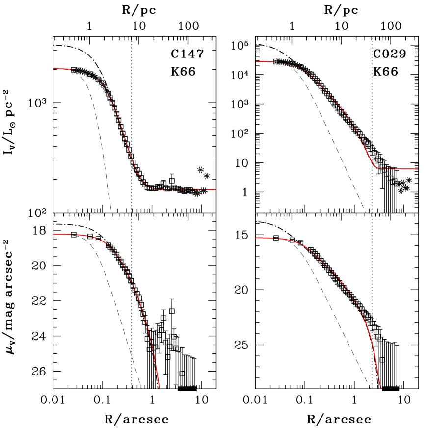
Figure 4: Examples of King (1966) model fits to two clusters in our sample: the fairly average C147 (left panels), and the very bright C029 (right panels), which has a large halo not well described by this standard model (cf. Paper I, ). Dashed curves trace the PSF intensity profile; bold dash-dot curves, the unconvolved best-fit model (with background added in the upper panels but not in the lower ones); and solid (red) curves, the PSF-convolved best fits. In each panel the lower $x$-axis is marked in arcsec and the upper $x$-axis in parsec. Vertical dotted lines mark the radius where the intrinsic cluster intensity is equal to the best-fit background. See text for more details.

The top panels of Figure 4 show the intensity versus radius profiles output from ELLIPSE for each cluster, after our conversion from $F606W$ to extinction-corrected $V$, described in §2, but before subtracting a constant background. The lower panels of the figure show the intensity profiles after subtracting the fitted backgrounds and converting to surface brightness, $\mu_{V}=26.402-2.5\,\log(I_{V}/L_{\odot}\,{\rm pc}^{-2})$. In all panels, the lower $x$-axis marks the projected radius $R$ in arcsec and the upper $x$-axis gives the equivalent scale in pc. The dashed curves falling steeply towards large $R$ show the (arbitrarily normalized) shape of the PSF in equation (3). The bold, dot-dash curves are the intrinsic (unconvolved) best-fit King (1966) models, with an added background in the upper panels but not in the lower panels. The solid (red) lines are the PSF-convolved models. Open squares are data points that were included in the least-squares model fitting, i.e., those flagged as OK in Table 3. Asterisks in the upper panels are points that were not used to constrain the fits (flagged as BAD, SAT, or DEP in Table 3); they have been omitted altogether from the lower plots. The dotted vertical lines in all four panels are at the radius in each cluster where the intrinsic model intensity is equal to the fitted background level. For radii larger than this, the observed intensities are at least 50% background according to the modeling. Points with intensities below the subtracted backgrounds are represented in the lower panels by solid points placed on the lower $x$-axes, with errorbars extending upwards.

The plots of the average C147 in Figure 4 are typical of the results for most of the clusters in our sample, in the sense that our derived intensity profiles extend to large enough radius that a constant background level has been reached. In this majority of cases, our procedure of fitting for the background at the same time as the intrinsic model parameters is very robust, with the same $I_{\rm bkg}$ estimated assuming any one of the three intrinsic cluster models discussed in §3.2. C147 is further typical of many moderate- and low-brightness objects with $L\la 10^{5}\,L_{\odot}$, in that the local “sky” level dominates any cluster signal outside of just a few intrinsic effective radii. Deviations of the data from the best-fit models in any of our five families occur mostly in this region of noise, and thus there is little difference in the overall quality of fit (and no large changes in the derived cluster parameters) from one type of model to another.

By contrast, the plots of C029 in Figure 4 show an interesting phenomenon that is seen in most of the very bright clusters in our sample. As we also mentioned above, it is clear here that a King (1966) model is simply not a good description of the data. One way of expressing this is to note the systematic excess of measured intensity over the best-fit model at radii $R\ga 1\arcsec\simeq 18$ pc, or about 3.5 fitted half-light radii. In order to minimize $\chi^{2}$ in this case, the fitted background intensity is spuriously high, coming in at roughly the average level of the outermost datapoints but failing utterly to reflect the clear, continual decreasing density profile of the real cluster. A stronger way of stating this “problem” is that any King (1966) model is too concave to match the data for this cluster: the model does not have the shape of the observed surface-brightness profile even at intermediate radii, outside of the PSF-blurred core but inside of where the fitted background level is reached.

Either way, on the basis of this failure of the standard King (1966) models, Paper I identified C029 and 5 other clusters similar to it as showing possible evidence for “extratidal light.” We have now found several other examples like this, but we have also fit them with alternate structural models that have intrinsically more extended haloes by construction. We generally find that the Wilson models for such objects return lower fitted background levels, different global cluster parameters such as $R_{h}$ and $L_{\rm tot}$, and often drastically smaller $\chi^{2}$ values. It would appear that the “excess” light implied by King (1966) model fits to some large clusters is likely a symptom of generic shortcomings in the model itself—the theoretical basis for it is weak in the low-density and unrelaxed farthest reaches of cluster envelopes—rather than the signature of genuine tidal debris. McLaughlin & van der Marel (2005) reached a similar conclusion after comparing King (1966) and Wilson fits to more than 150 old and young massive clusters in the Milky Way and some of its satellites.

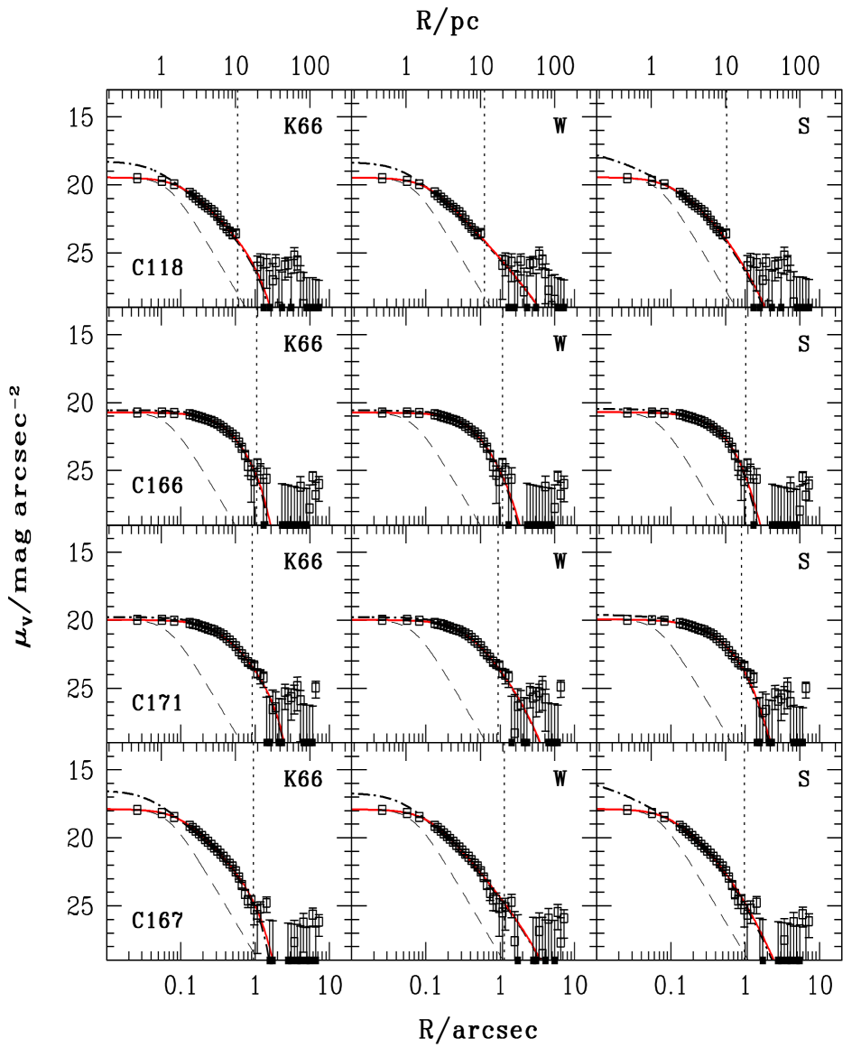
Figure 5: Examples of King (1966), Wilson, and Sérsic model fits to 8 globular clusters in NGC 5128. Results are shown in the same background-subtracted format as the lower panels of Figure 4, with all points and curves having the same meaning here as there. Clustercentric distance is marked in arcsec along the lower $x$-axis in each panel, and in parsec along the upper $x$-axis. Clusters are presented in order of increasing brightness from top to bottom: $M_{V}=-6.0$ for C118, $M_{V}=-6.5$ for C166, $M_{V}=-7.4$ for C171, $M_{V}=-7.4$ for C167, $M_{V}=-8.7$ for C113, $M_{V}=-8.8$ for F1GC15, $M_{V}=-10.2$ for C029, and $M_{V}=-11.2$ for C007 (all magnitudes from King 1966 model fits and assuming $D=3.8$ Mpc).

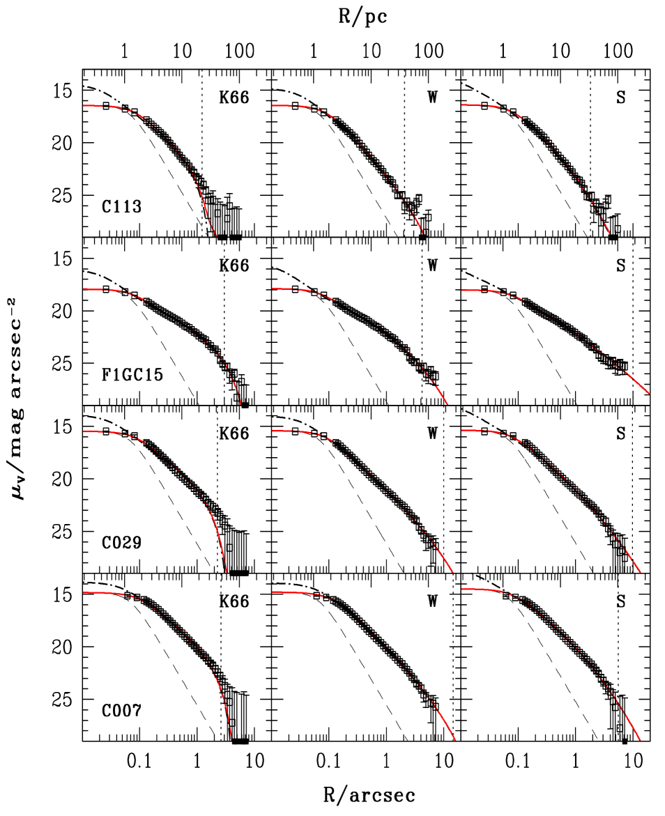
Figure 6: continued

Examples of King (1966), Wilson, and Sérsic model fits to 8 globular clusters in NGC 5128. Results are shown in the same background-subtracted format as the lower panels of Figure 4, with all points and curves having the same meaning here as there. Clustercentric distance is marked in arcsec along the lower $x$-axis in each panel, and in parsec along the upper $x$-axis. Clusters are presented in order of increasing brightness from top to bottom: $M_{V}=-6.0$ for C118, $M_{V}=-6.5$ for C166, $M_{V}=-7.4$ for C171, $M_{V}=-7.4$ for C167, $M_{V}=-8.7$ for C113, $M_{V}=-8.8$ for F1GC15, $M_{V}=-10.2$ for C029, and $M_{V}=-11.2$ for C007 (all magnitudes from King 1966 model fits and assuming $D=3.8$ Mpc).

Table 7: Derived structural and photometric parameters from 147 profiles of 131 GCs in NGC 5128

Name	Detector	Model	$\log\,r_{\rm tid}$	$\log\,R_{c}$	$\log\,R_{h}$	$\log\,(R_{h}/R_{c})$	$\log\,I_{0}$	$\log\,j_{0}$	$\log\,L_{V}$	$V_{\rm tot}$	$\log\,I_{h}$
			[pc]	[pc]	[pc]		[$L_{\odot,V}\,{\rm pc}^{-2}$]	[$L_{\odot,V}\,{\rm pc}^{-3}$]	[$L_{\odot,V}$]	[mag]	[$L_{\odot,V}\,{\rm pc}^{-2}$]
(1)	(2)	(3)	(4)	(5)	(6)	(7)	(8)	(9)	(10)	(11)	(12)
AAT111563	WFC/F606	K66	$1.50^{+0.01}_{-0.03}$	$0.035^{+0.022}_{-0.012}$	$0.468^{+0.005}_{-0.010}$	$0.433^{+0.017}_{-0.032}$	$3.87^{+0.02}_{-0.03}$	$3.53^{+0.03}_{-0.05}$	$5.05^{+0.02}_{-0.02}$	$20.10^{+0.05}_{-0.05}$	$3.32^{+0.02}_{-0.02}$
		W	$2.03^{+0.08}_{-0.08}$	$0.089^{+0.015}_{-0.016}$	$0.486^{+0.017}_{-0.014}$	$0.396^{+0.033}_{-0.029}$	$3.82^{+0.03}_{-0.03}$	$3.42^{+0.04}_{-0.04}$	$5.07^{+0.02}_{-0.02}$	$20.05^{+0.06}_{-0.06}$	$3.30^{+0.03}_{-0.03}$
		S	$\infty$	$-0.875^{+0.131}_{-0.145}$	$0.478^{+0.010}_{-0.009}$	$1.353^{+0.155}_{-0.140}$	$4.42^{+0.09}_{-0.08}$	$4.23^{+0.21}_{-0.19}$	$5.05^{+0.02}_{-0.02}$	$20.10^{+0.05}_{-0.05}$	$3.30^{+0.02}_{-0.02}$
AAT113992	WFC/F606	K66	$1.58^{+0.07}_{-0.04}$	$0.144^{+0.008}_{-0.011}$	$0.560^{+0.041}_{-0.023}$	$0.416^{+0.051}_{-0.030}$	$3.70^{+0.02}_{-0.02}$	$3.25^{+0.03}_{-0.02}$	$5.08^{+0.04}_{-0.03}$	$20.02^{+0.07}_{-0.09}$	$3.16^{+0.03}_{-0.05}$
		W	$2.64^{+0.31}_{-0.27}$	$0.151^{+0.012}_{-0.011}$	$0.749^{+0.144}_{-0.097}$	$0.599^{+0.155}_{-0.109}$	$3.69^{+0.02}_{-0.02}$	$3.24^{+0.03}_{-0.03}$	$5.21^{+0.08}_{-0.06}$	$19.69^{+0.16}_{-0.21}$	$2.92^{+0.13}_{-0.21}$
		S	$\infty$	$-0.395^{+0.071}_{-0.072}$	$0.528^{+0.016}_{-0.015}$	$0.923^{+0.088}_{-0.086}$	$4.03^{+0.04}_{-0.04}$	$3.45^{+0.10}_{-0.09}$	$5.05^{+0.02}_{-0.02}$	$20.11^{+0.06}_{-0.06}$	$3.19^{+0.03}_{-0.03}$
AAT115339	WFC/F606	K66	$1.33^{+0.02}_{-0.01}$	$-1.752^{+0.190}_{-0.214}$	$0.376^{+0.003}_{-0.000}$	$2.127^{+0.216}_{-0.190}$	$6.07^{+0.20}_{-0.17}$	$7.52^{+0.42}_{-0.36}$	$5.19^{+0.02}_{-0.02}$	$19.76^{+0.05}_{-0.05}$	$3.64^{+0.02}_{-0.02}$
		W	$2.01^{+0.20}_{-0.16}$	$-0.033^{+0.035}_{-0.040}$	$0.397^{+0.044}_{-0.028}$	$0.430^{+0.084}_{-0.062}$	$4.19^{+0.05}_{-0.04}$	$3.92^{+0.09}_{-0.08}$	$5.22^{+0.03}_{-0.03}$	$19.67^{+0.07}_{-0.08}$	$3.63^{+0.04}_{-0.06}$
		S	$\infty$	$-1.246^{+0.173}_{-0.177}$	$0.384^{+0.009}_{-0.009}$	$1.630^{+0.186}_{-0.182}$	$4.93^{+0.11}_{-0.11}$	$5.08^{+0.26}_{-0.25}$	$5.20^{+0.02}_{-0.02}$	$19.72^{+0.05}_{-0.05}$	$3.64^{+0.02}_{-0.02}$

A machine-readable version of the full Table 7 is available online (http://www.astro.keele.ac.uk/$\sim$dem/clusters.html) or upon request from the first author. Only a short extract from it is shown here, for guidance regarding its form and content.

Table 8: Derived dynamical parameters from 147 profiles of 131 GCs in NGC 5128

Name	Detector	$\Upsilon_{V}^{\rm pop}$	Model	$\log\,M_{\rm tot}$	$\log\,E_{b}$	$\log\,\Sigma_{0}$	$\log\,\rho_{0}$	$\log\,\Sigma_{h}$	$\log\,\sigma_{{\rm p},0}$	$\log\,v_{{\rm esc},0}$	$\log\,t_{\rm rh}$	$\log\,f_{0}$
		[$M_{\odot}\,L_{\odot,V}^{-1}$]		[$M_{\odot}$]	[erg]	[$M_{\odot}\,{\rm pc}^{-2}$]	[$M_{\odot}\,{\rm pc}^{-3}$]	[$M_{\odot}\,{\rm pc}^{-2}$]	[km s-1]	[km s-1]	[yr]
(1)	(2)	(3)	(4)	(5)	(6)	(7)	(8)	(9)	(10)	(11)	(12)	(13)
AAT111563	WFC/F606	$1.939^{+0.239}_{-0.240}$	K66	$5.34^{+0.05}_{-0.06}$	$50.62^{+0.08}_{-0.09}$	$4.16^{+0.06}_{-0.07}$	$3.82^{+0.06}_{-0.08}$	$3.60^{+0.06}_{-0.06}$	$0.836^{+0.027}_{-0.030}$	$1.421^{+0.027}_{-0.031}$	$8.92^{+0.03}_{-0.03}$	$0.079^{+0.038}_{-0.056}$
			W	$5.36^{+0.06}_{-0.06}$	$50.62^{+0.08}_{-0.09}$	$4.11^{+0.06}_{-0.06}$	$3.71^{+0.06}_{-0.07}$	$3.59^{+0.06}_{-0.07}$	$0.839^{+0.027}_{-0.030}$	$1.427^{+0.027}_{-0.031}$	$8.96^{+0.04}_{-0.04}$	$-0.049^{+0.045}_{-0.045}$
			S	$5.34^{+0.05}_{-0.06}$	$50.62^{+0.08}_{-0.09}$	$4.70^{+0.10}_{-0.10}$	$4.52^{+0.21}_{-0.19}$	$3.58^{+0.06}_{-0.06}$	$0.797^{+0.028}_{-0.032}$	$1.470^{+0.028}_{-0.031}$	$8.94^{+0.03}_{-0.03}$	$1.134^{+0.287}_{-0.255}$
AAT113992	WFC/F606	$2.914^{+0.431}_{-0.423}$	K66	$5.55^{+0.07}_{-0.07}$	$50.94^{+0.09}_{-0.10}$	$4.16^{+0.06}_{-0.07}$	$3.71^{+0.07}_{-0.07}$	$3.63^{+0.07}_{-0.09}$	$0.893^{+0.032}_{-0.036}$	$1.476^{+0.032}_{-0.036}$	$9.16^{+0.08}_{-0.05}$	$-0.197^{+0.042}_{-0.040}$
			W	$5.68^{+0.10}_{-0.09}$	$51.01^{+0.10}_{-0.11}$	$4.16^{+0.06}_{-0.07}$	$3.70^{+0.07}_{-0.07}$	$3.38^{+0.15}_{-0.22}$	$0.895^{+0.032}_{-0.036}$	$1.499^{+0.032}_{-0.036}$	$9.50^{+0.25}_{-0.17}$	$-0.215^{+0.043}_{-0.046}$
			S	$5.51^{+0.06}_{-0.07}$	$50.92^{+0.09}_{-0.10}$	$4.49^{+0.07}_{-0.08}$	$3.91^{+0.10}_{-0.10}$	$3.66^{+0.07}_{-0.07}$	$0.877^{+0.032}_{-0.036}$	$1.507^{+0.032}_{-0.036}$	$9.10^{+0.04}_{-0.05}$	$0.158^{+0.136}_{-0.133}$
AAT115339	WFC/F606	$2.015^{+0.238}_{-0.235}$	K66	$5.49^{+0.05}_{-0.06}$	$51.08^{+0.07}_{-0.08}$	$6.37^{+0.21}_{-0.18}$	$7.82^{+0.42}_{-0.37}$	$3.94^{+0.05}_{-0.06}$	$1.047^{+0.028}_{-0.029}$	$1.767^{+0.028}_{-0.030}$	$8.85^{+0.03}_{-0.03}$	$3.482^{+0.435}_{-0.391}$
			W	$5.53^{+0.06}_{-0.06}$	$51.05^{+0.07}_{-0.08}$	$4.49^{+0.07}_{-0.07}$	$4.22^{+0.10}_{-0.09}$	$3.94^{+0.06}_{-0.08}$	$0.972^{+0.026}_{-0.029}$	$1.563^{+0.028}_{-0.030}$	$8.89^{+0.08}_{-0.06}$	$0.067^{+0.088}_{-0.080}$
			S	$5.51^{+0.05}_{-0.06}$	$51.05^{+0.07}_{-0.08}$	$5.24^{+0.12}_{-0.12}$	$5.38^{+0.26}_{-0.25}$	$3.94^{+0.05}_{-0.06}$	$0.913^{+0.029}_{-0.031}$	$1.616^{+0.027}_{-0.030}$	$8.87^{+0.03}_{-0.03}$	$1.734^{+0.355}_{-0.343}$

A machine-readable version of the full Table 8 is available online (http://www.astro.keele.ac.uk/$\sim$dem/clusters.html) or upon request from the first author. Only a short extract from it is shown here, for guidance regarding its form and content.

Table 9: Galactocentric radii and $\kappa$-space parameters from 147 profiles of 131 GCs in NGC 5128

Name	Detector	$R_{\rm gc}$	Model	$\kappa_{m,1}$	$\kappa_{m,2}$	$\kappa_{m,3}$
		[kpc]
(1)	(2)	(3)	(4)	(5)	(6)	(7)
AAT111563	WFC/F606	11.93	K66	$-0.608^{+0.039}_{-0.044}$	$4.660^{+0.068}_{-0.075}$	$0.346^{+0.002}_{-0.003}$
			W	$-0.591^{+0.040}_{-0.044}$	$4.642^{+0.070}_{-0.079}$	$0.349^{+0.004}_{-0.003}$
			S	$-0.657^{+0.039}_{-0.044}$	$4.607^{+0.070}_{-0.078}$	$0.306^{+0.008}_{-0.009}$
AAT113992	WFC/F606	4.26	K66	$-0.462^{+0.052}_{-0.052}$	$4.689^{+0.084}_{-0.105}$	$0.345^{+0.005}_{-0.002}$
			W	$-0.326^{+0.110}_{-0.084}$	$4.410^{+0.168}_{-0.246}$	$0.380^{+0.035}_{-0.019}$
			S	$-0.507^{+0.045}_{-0.050}$	$4.714^{+0.081}_{-0.091}$	$0.328^{+0.003}_{-0.004}$
AAT115339	WFC/F606	3.82	K66	$-0.375^{+0.039}_{-0.041}$	$5.147^{+0.065}_{-0.071}$	$0.447^{+0.011}_{-0.006}$
			W	$-0.467^{+0.050}_{-0.046}$	$5.070^{+0.075}_{-0.097}$	$0.352^{+0.012}_{-0.006}$
			S	$-0.558^{+0.038}_{-0.042}$	$5.032^{+0.068}_{-0.074}$	$0.289^{+0.011}_{-0.012}$

A machine-readable version of the full Table 9 is available online (http://www.astro.keele.ac.uk/$\sim$dem/clusters.html) or upon request from the first author. Only a short extract from it is shown here, for guidance regarding its form and content.

Figure 5 compares the fits of King (1966), Wilson, and Sérsic models to the background-subtracted, $V$-band surface-brightness profiles of eight more globulars in NGC 5128, displayed in order of increasing total cluster brightness; C029 appears in the second-last row of this figure. The curves and points in every plot have the same meaning as in the lower panels of Figure 4.

The first cluster shown in Figure 5, C118, is one of the faintest in our sample ($M_{V}=-6.0$, or $L_{V}\simeq 2.1\times 10^{4}\,L_{\odot}$ according to the King 1966 model fit shown) and has an effective (or half-light) radius of $R_{h}\simeq 3$–4 pc—typical of most known globular clusters in any galaxy—depending slightly on the model fit. The next cluster, C166, is similarly faint ($M_{V}=-6.5$, or $L_{V}\simeq 3.4\times 10^{4}\,L_{\odot}$) but significantly more extended: $R_{h}\simeq 6.5$ pc for any of the models fit. This conclusion is clearly not influenced by the PSF; in fact, these plots demonstrate that almost all of our cluster candidates are very well resolved indeed.

The next two clusters, C171 and C167, both have the same brightness (fitted $M_{V}\simeq-7.4$ or $L_{V}\simeq 7.8\times 10^{4}\,L_{\odot}$, essentially at the expected peak of the GC luminosity function), but the first is significantly more diffuse than the second: $R_{h}\simeq 8$ pc versus $R_{h}\simeq 3$ pc. Evidently, there is substantial scatter in any size-mass relation that one might try to explore for average and faint globulars in NGC 5128. This is reminiscent of the well-known situation in the Milky Way GC system, and we return to the point in our analysis of structural correlations in Paper IV.

As we discussed in connection with C147 above, the three model fits to the globulars in this first half of Figure 5 are all very similar: the estimates of the sky level $I_{\rm bkg}$ are all about the same, as are the total fitted luminosities, effective radii, and other cluster parameters. The minimum $\chi^{2}$ for the different models are also very similar for any one cluster, and there is no sign that the extended Wilson or Sérsic haloes are systematically either preferred over or bettered by the standard King (1966) structure. It is worth noting that the Sérsic model fits can return significantly smaller core radii and brighter intrinsic central surface brightnesses than the other models; but at some level this simply points to a limitation of the data, since the unavoidable PSF convolution effectively erases the intrinsically cuspy inner structures of $n>1$ Sérsic models, which might be disallowed by much higher-resolution data.

In the second half of Figure 5, the clusters C113 and F1GC15 are both taken from the bright side of the GC luminosity function in NGC 5128 ($M_{V}=-8.7$ and $M_{V}=-8.8$), and once again one is much larger than the other ($R_{h}=2.5$ pc against $R_{h}=16.5$ pc in the most conservative, King 1966 model fits). Now, however, the quality of fit differs significantly between the different models. In C113, the minimum $\chi^{2}$ is nearly 7 times smaller for the Wilson model versus King (1966), and just over 5 times smaller for Sérsic versus King (1966). For F1GC15, the Wilson fit has a $\chi^{2}$ about 20% larger than the King (1966) fit (so the latter is formally somewhat better, but only marginally so), while the Sérsic model is effectively ruled out with a minimum $\chi^{2}$ more than 6 times larger than the King (1966) model.

The last two clusters illustrated here are C029—confirming that this object is much better fit by a Wilson model than a King (1966) model, and also showing that the former does better than a Sérsic model—and C007, which is the brightest GC in our sample ($M_{V}=-11.2$, or $L_{V}=2.6\times 10^{6}\,L_{\odot}$ from a King 1966 model fit). It too is better fit by a Wilson model than by either of the other two.

We note again that, because the extended-halo structure of all the bright clusters in Figure 5 is poorly fit by the relatively compact King (1966) models, the fitted background intensity is noticeably, but spuriously, higher in the leftmost panels than in the other columns.

We will return to the question of which model best fits the majority of GCs in NGC 5128, in §4.4 below. First, we present a number of physical cluster properties derived within the framework of each of the model fits summarized in Table 6.

4.2 Derived quantities

Table 7 contains a number of other cluster properties derived from the basic fit parameters given in Table 6. Columns following the GC name, detector/filter combination, and fitted model are:

Column (4): $\log\,r_{t}=c+\log\,r_{0}$, the model tidal radius in pc, which is always infinite for Sérsic models.

Column (5): $\log\,R_{c}$, the projected core radius of the model fitting a cluster, in units of pc. This is defined by $I(R_{c})=I_{0}/2$, or $\mu(R_{c})\simeq\mu_{0}+0.753$ and is not necessarily the same as the radial scale $r_{0}$ in Table 6, except for Sérsic models.

Column (6): $\log R_{h}$, the projected half-light, or effective, radius of a model. Half the total cluster luminosity is projected within $R_{h}$. It is related to $r_{0}$ by one-to-one functions of $W_{0}$ (or $c$) or $n$ and is reported here in units of pc.

Column (7): $\log\,(R_{h}/R_{c})$, a measure of cluster concentration that is somewhat more model-independent than $c$ or $n$, in that it is generically well defined in observational terms and its physical meaning is always the same (cf. our earlier discussion in §3.2). We consider it a more suitable quantity to use when intercomparing the overall properties of clusters that may not all be fit by the same kind of model.

Column (8): $\log\,I_{0}$, the best-fit central ($R=0$) luminosity surface density in the $V$ band, in units of $L_{\odot,V}\,{\rm pc}^{-2}$. This is obtained from the fitted central surface brightness in Column (11) of Table 6, by first applying the “$V$-colour” correction in Column (4) of that table to obtain the central $\mu_{V,0}$, and then using the definition $\log\,I_{V}=0.4\,(26.402-\mu_{V})$, where the zeropoint corresponds to a solar absolute magnitude of $M_{\odot,V}=+4.83$.

Column (9): $\log\,j_{0}$, the $V$-band luminosity volume density ($L_{\odot,V}\,{\rm pc}^{-3}$) at $r=0$ for King (1966) and Wilson models but at the three-dimensional radius $r=r_{0}$ for Sérsic models. In the first two cases, $j_{0}={\cal J}I_{0}/r_{0}$ where ${\cal J}$ is a smooth, model-dependent function of $W_{0}$ or $c$, which we have calculated numerically. For Sérsic models, as we discussed in §3.2, the unprojected density is infinite as $r\rightarrow 0$ when $n\geq 1$, and thus we only quote $j_{0}\equiv j(r_{0})$ for any fitted $n$. This finite quantity is related to the quotient $I_{0}/r_{0}$ by a well-defined function of $n$, which we have again computed numerically.

Column (10): $\log\,L_{V}$, the total integrated model luminosity in the $V$ band. It is related to the product $I_{0}r_{0}^{2}$ by model-dependent functions of $W_{0}$ or $c$, or $n$.

Column (11): $V_{\rm tot}=4.83-2.5\,\log\,(L_{V}/L_{\odot})+5\,\log\,(D/10\,{\rm pc})$, the total, extinction-corrected apparent $V$-band magnitude of a model cluster, assuming $D=3.8$ Mpc.

Column (12): $\log I_{h}\equiv\log\,(L_{V}/2\pi R_{h}^{2})$, the $V$-band luminosity surface density averaged over the half-light or effective radius, in units of $L_{\odot,V}\,{\rm pc}^{-2}$. The $V$ surface brightness averaged over $R_{h}$ is $\langle\mu_{V}\rangle_{h}\equiv 26.402-2.5\,\log\,(I_{h}/L_{\odot,V}\,{\rm pc}^{-2})$.

The uncertainties on all of these derived parameters have been estimated from the $\chi^{2}$ re-scaling procedure described after Table 6. If the distance $D$ to NGC 5128 is different from our adopted 3.8 Mpc, the quantities in Table 7 will change according to: $r_{\rm tid}$, $R_{c}$, and $R_{h}$ all $\propto D$; $I_{0}$ and $I_{h}$ independent of $D$; $j_{0}\propto D^{-1}$; and $L_{V}\propto D^{2}$.

Table 8 next lists a number of cluster properties derived from the structural parameters already given plus a mass-to-light ratio. The first two columns of this table contain the name of each cluster and the combination of detector/filter for our observations of it, as usual. Column (3) lists the $V$-band mass-to-light ratio that we have adopted for each object from the analysis in §3.1, assuming for definiteness an age of 13 Gyr for all clusters. The errorbars on $\Upsilon_{V}^{\rm pop}$ in Table 8 are larger than those in the 13-Gyr column of Table 5, as we allow now for a $\pm 2$-Gyr uncertainty in age on top of the previously tabulated uncertainties in [Fe/H]. The remaining entries in Table 8 are, for the best fit of each model to every cluster:

Column (5): $\log\,M_{\rm tot}=\log\,\Upsilon_{V}^{\rm pop}+\log\,L_{V}$, the integrated model mass in solar units, with $\log\,L_{V}$ taken from Column (10) of Table 7.

Column (6): $\log\,E_{b}$, the integrated binding energy in ergs, defined through $E_{b}\equiv-(1/2)\int_{0}^{r_{t}}4\pi r^{2}\rho\phi\,dr$. Here the minus sign makes $E_{b}$ positive for gravitationally bound objects, and $\phi(r)$ is the potential generated (through Poisson’s equation) by the model mass distribution $\rho(r)$. $E_{b}$ can be written in terms of the fitted central luminosity density $j_{0}$; scale radius $r_{0}$; a model-dependent function of $W_{0}$ or $c$, or $n$; and $\Upsilon_{V}^{\rm pop}$. A more detailed outline of this procedure for King (1966) models may be found in McLaughlin (2000), which we have followed closely to evaluate $E_{b}$ for our other model fits as well.

Column (7): $\log\,\Sigma_{0}=\log\,\Upsilon_{V}^{\rm pop}+\log\,I_{0}$, the central surface mass density in the model, in units of $M_{\odot}\,{\rm pc}^{-2}$.

Column (8): $\log\,\rho_{0}=\log\,\Upsilon_{V}^{\rm pop}+\log\,j_{0}$, the central volume density in units of $M_{\odot}\,{\rm pc}^{-3}$ (except for Sérsic models, where $\rho_{0}$ is the density at the three-dimensional radius $r_{0}$).

Column (9): $\log\,\Sigma_{h}=\log\,\Upsilon_{V}^{\rm pop}+\log\,I_{h}$, the surface mass density averaged over the inner effective radius $R_{h}$, in units of $M_{\odot}\,{\rm pc}^{-2}$.

Column (10): $\log\,\sigma_{{\rm p},0}$, the predicted line-of-sight velocity dispersion at the cluster centre for King (1966) and Wilson models, but at $r_{0}=R_{c}$ for Sérsic models, in km s^-1. The solution of Poisson’s and Jeans’ equations for any model yields a dimensionless $\sigma_{{\rm p},0}/\sigma_{0}$, and with $\sigma_{0}$ given by the fitted $r_{0}$ and $\rho_{0}=\Upsilon_{V}^{\rm pop}j_{0}$ through equation (9) or (10), the predicted observable dispersion follows immediately.

Column (11): $\log\,v_{{\rm esc},0}$, the predicted central “escape” velocity in km s^-1. A star moving out from the centre of a cluster with speed $v_{{\rm esc},0}$ will just come to rest at infinity. In general, then,

$$v_{{\rm esc},0}^{2}/\sigma_{0}^{2}=2\left[W_{0}+GM_{\rm tot}/r_{t}\sigma_{0}^{2}\right]\ .$$

A (finite) dimensionless $W_{0}$ is associated with any $n>0$ for Sérsic models by solving Poisson’s equation with $\phi\rightarrow 0$ in the limit $r\rightarrow\infty$. The second term on the right-hand side of the definition of $v_{{\rm esc},0}$ vanishes for Sérsic models, in which $r_{t}\rightarrow\infty$.

Column (12): $\log\,t_{\rm rh}$, the two-body relaxation time at the model projected half-mass radius, in years. This is estimated as

$$t_{\rm rh}=\frac{2.06\times 10^{6}\ {\rm yr}}{\ln\left(0.4M_{\rm tot}/m_{\star}\right)}\frac{M_{\rm tot}^{1/2}R_{h}^{3/2}}{m_{\star}}$$

(Binney & Tremaine, 1987, eq. 8-72), if $m_{\star}$ (the average stellar mass in a cluster) and $M_{\rm tot}$ are both in solar units and $R_{h}$ is in pc. We have evaluated this timescale assuming an average $m_{\star}=0.5\,M_{\odot}$ in all clusters.

Column (13): $\log f_{0}\equiv\log\,\left[\rho_{0}/(2\pi\sigma_{c}^{2})^{3/2}\right]$, a measure of the model’s “central” phase-space density in units of $M_{\odot}\,{\rm pc}^{-3}\,({\rm km\ s^{-1}})^{-3}$. In this expression, $\sigma_{c}$ refers to the central one-dimensional velocity dispersion not projected along the line of sight. The ratio $\sigma_{c}/\sigma_{0}$ is obtained for King (1966) and Wilson models from the solution of the Poisson and Jeans equations for given $W_{0}$ or $c$, and $\sigma_{0}$ is known from equation (9). This procedure breaks down for Sérsic models in general, since the unprojected $\rho\rightarrow\infty$ and $\sigma\rightarrow 0$ as $r\rightarrow 0$ for $n\geq 1$. As before, then, for these models we instead calculate $f_{0}$ at the three-dimensional radius $r=r_{0}$. In any case, with the central relaxation time $t_{\rm rc}$ of a cluster defined as in equation (8-71) of Binney & Tremaine (1987), taking an average stellar mass of $m_{\star}=0.5\,M_{\odot}$ and a typical Coulomb logarithm $\ln\Lambda\approx 12$ leads to the approximate relation $\log\,(t_{\rm rc}/{\rm yr})\simeq 8.28-\log\,f_{0}$.

The uncertainties in these quantities are estimated from their variations around the minimum of $\chi^{2}$ on the model grids we fit, as above, but now combined in quadrature with the uncertainties in the population-synthesis model $\Upsilon_{V}^{\rm pop}$. Note that if $\Upsilon_{V}^{\rm pop}$ is changed to any other value for any cluster, or if any distance other than $D=3.8$ Mpc is adopted for NGC 5128, the properties in Table 8 scale as $M_{\rm tot}\propto\Upsilon\,D^{2}$; $E_{b}\propto\Upsilon^{2}\,D^{3}$; $\Sigma_{0}\propto\Upsilon\,D^{0}$ and $\Sigma_{h}\propto\Upsilon\,D^{0}$; $\rho_{0}\propto\Upsilon\,D^{-1}$; $\sigma_{{\rm p},0}\propto\Upsilon^{1/2}\,D^{1/2}$ and $v_{{\rm esc},0}\propto\Upsilon^{1/2}\,D^{1/2}$; $t_{\rm rh}\propto\Upsilon^{1/2}\,D^{5/2}$; and $f_{0}\propto\Upsilon^{-1/2}\,D^{-5/2}$.

Table 9 provides the last few parameters required to construct the fundamental plane of globular clusters in NGC 5128, under any of the equivalent formulations of it in the literature. The first of these remaining parameters is the projected galactocentric distance $R_{\rm gc}$, in kpc, of each cluster. This is listed in Column (3) of Table 9, following the cluster name and detector/filter combination. It is obtained from the angular $R_{\rm gc}$ given in Tables 1 and 2 of Paper II, assuming $D=3.8$ Mpc as always.

The last three columns of Table 9 give analogues of the so-called $\kappa$ parameters introduced by Bender, Burstein, & Faber (1992), who define an orthonormal “coordinate” system based on the three main luminosity observables of galaxies. Similarly to them, but in terms of mass-based quantities instead, we define

$$\begin{array}[]{rcl}\kappa_{m,1}&\equiv&(\log\,\sigma_{{\rm p},0}^{2}+\log\,R_{h})/\sqrt{2}\\ \kappa_{m,2}&\equiv&(\log\,\sigma_{{\rm p},0}^{2}+2\,\log\Sigma_{h}-\log\,R_{h})/\sqrt{6}\\ \kappa_{m,3}&\equiv&(\log\,\sigma_{{\rm p},0}^{2}-\log\,\Sigma_{h}-\log\,R_{h})/\sqrt{3}\\ \end{array}$$ (13)

which differ from the $\kappa$’s in Bender, Burstein, & Faber (and Burstein et al., 1997) only in our use of the average mass surface density $\Sigma_{h}$ rather than the luminosity surface density $I_{h}=\Sigma_{h}/\Upsilon_{V}$. The main reason for doing this is to facilitate the comparison of fundamental planes for young and old star clusters, by removing the influence of age on $I_{h}$ for two objects of similar mass and size. It similarly avoids the influence that any metallicity dependence in $\Upsilon_{V}$ has on a luminosity-based fundamental plane.

In equation (13), $\kappa_{m,1}\leftrightarrow\log\,(\sigma_{{\rm p},0}^{2}R_{h})$ is related to the total mass of a system, and $\kappa_{m,3}\leftrightarrow\log\,(\sigma_{{\rm p},0}^{2}R_{h}/M_{\rm tot})$ contains the exact details of this relationship—that is, information on the internal density profile $\rho(r)$. In fact, the mass-based $\kappa_{m,3}$ can be viewed as a replacement for King- or Wilson-model concentrations $c$ or Sérsic-model indices $n$, or any other model-specific shape parameter. As such, any trends involving $\kappa_{m,3}$ are directly of relevance to questions concerning cluster (non)homology. The definition of $\kappa_{m,2}\leftrightarrow\log\,(\Sigma_{h}^{3})$ is chosen to make the three $\kappa_{m}$ axes space mutually orthogonal in the parameter space of $(\sigma_{{\rm p},0}^{2},R_{h},\Sigma_{h})$.

In calculating $\kappa_{m,1}$, $\kappa_{m,2}$, and $\kappa_{m,3}$ for Table 9, we have used the $\sigma_{{\rm p},0}$ predicted in Table 8 (Column 7) by our adoption of population-synthesis mass-to-light ratios. Similarly, $\Sigma_{h}$ is taken from Column (9) of Table 8. As a result, our values for $\kappa_{m,3}$ are independent of $\Upsilon_{V}^{\rm pop}$. $R_{h}$ is taken from Table 7 but put in units of kpc rather than pc, for better compatibility with the original, galaxy-oriented definitions of Bender, Burstein, & Faber (1992).

4.3 Consistency checks

Figure 7: Comparison of concentration parameters, intrinsic radii, total luminosities, and intrinsic central surface brightnesses for fits of isotropic Wilson (1975) models to each of the two independent intensity profiles measured for 15 of the GC candidates listed in Table 1 (not including the possible star, C156). In the upper-right panel, filled symbols refer to estimates of the model scale radii $r_{0}$ for the clusters, while open circles refer to the effective (projected half-light) radii $R_{h}$.

There are two ways in which we can assess the internal consistency of the various model fits we have performed.

First, Figure 7 compares some of the main parameters obtained from Wilson fits to the 15 clusters in Table 1, for which we have two independent surface-brightness profiles measured on two different main ACS fields. (We have excluded the object C156 from this comparison; cf. Table 2.)

The $x$-axis of every panel in Figure 7 marks the parameter value measured for the clusters in the survey target fields where they lie closest to the chip centre (the fields highlighted in bold in Table 1). The $y$-axes then measure the parameter values found in the ACS field where the clusters lie further from the centre. There is evidently no substantial or systematic scatter around the line of equality drawn in each case. For these Wilson fits we find that the average and rms scatter in the difference of fitted concentrations is (in the sense [off-centre] minus [central]) $\langle\delta c\rangle=-0.02\pm 0.08$, as compared to an rms errorbar of $\pm\,0.13$ on the individual $c$ values. For the scale and half-light radii, $\langle\delta(\log\,r_{0})\rangle=\langle\delta(\log\,R_{h})\rangle=0.01\pm 0.03$ dex, versus an rms fit uncertainty of about $\pm\,0.04$ dex in both cases. Finally, we have $\langle\delta(\log\,L_{V})\rangle=0\pm 0.01$ dex and $\langle\delta\mu_{V,0}\rangle=0.03\pm 0.11$ mag arcsec^-2, against rms errorbars of $\pm\,0.03$ dex and $\pm\,0.09$ mag arcsec^-2. Nearly identical results hold for comparisons of fitted King (1966) and Sérsic model parameters.

We conclude that any PSF variations over the ACS/WFC chip have not introduced any systematic errors into our model fitting, which assumed a single PSF shape in all cases. For all subsequent analyses, we include the clusters with double measurements by adopting the fit parameters obtained from the image on which the cluster is closest to the chip centre.

Figure 8: Comparison of total King (1966) and Wilson model $V$ magnitudes versus aperture or PSF estimates (extinction-corrected) from Paper II (cf. Harris, Harris, & Geisler, 2004), for 124 reliable GC candidates.

Second, Figure 8 shows the total apparent $V$-band magnitudes inferred from our King (1966) and Wilson model fits (from Column [11] of Table 4) to the $V$-band equivalents of Washington $T_{1}$ magnitudes estimated from ground-based aperture or PSF photometry and tabulated in Paper II (numbers taken originally from Harris, Harris, & Geisler 2004). To transform $T_{1}$ to $V$, we first corrected for extinction according to $A_{T1}=2.54\times E(B-V)=0.279$ mag for all clusters (Harris & Canterna, 1979), and then used the relationship $V_{\rm tot}=T_{1,0}+0.052+0.256\times(C-T_{1})_{0}$ from Paper I (see also Geisler 1996) given the de-reddened Washington colours in Paper II and our Table 4 above. We have excluded from this comparison the clusters C168, F1GC34, and F2GC14, for the reasons given in Table 2; the objects C145, C152, C156, which are likely foreground stars; and C177, which is probably a background galaxy.

For bright clusters with $V_{\rm tot}<20$ ($M_{V}<-7.9$), our model luminosities compare rather well in general to the aperture or PSF magnitudes; with $\delta V_{\rm tot}\equiv[V_{\rm tot}({\rm model})-V_{\rm tot}({\rm aperture\ or\ PSF})]$, we have $\langle\delta V_{\rm tot}\rangle=0\pm 0.13$ mag (rms) for the King (1966) model fits, and $\langle\delta V_{\rm tot}\rangle=-0.14\pm 0.18$ mag (rms) for Wilson fits. Both results are quite acceptable, considering (1) the number of steps involved in transforming either our models or the Washington photometry of Paper II and Harris, Harris, & Geisler (2004) to standard $V$ magnitudes; and (2) the fact that the aperture or PSF magnitudes are from analyses of ground-based data and limited to clustercentric radii of only $R\la 2\arcsec$–$3\arcsec$ (about 35–55 pc), which can easily miss up to $\sim\!0.2$ mag of cluster light (see Figure 5 above, and also the discussion in Harris, Harris, & Geisler 2004). The 0.15-mag offset between the average Wilson and King (1966) model magnitudes is a direct result of the fact that the latter models are generally too compact to fit the brightest clusters well and thus underestimate the true luminosity of the cluster haloes.

Fainter clusters with $V_{\rm tot}\ga 20$ according to the aperture or PSF measurements have $\delta V_{\rm tot}$ offsets that are on average $\simeq\!0.1$ mag brighter than for the brighter GCs, and that have a larger rms scatter about the average. This is due to our ability here (unlike in Harris, Harris, & Geisler 2004) to resolve all of these faint clusters and robustly to estimate and correct for the local background intensity around each of them. We thus view our present measurements of $V_{\rm tot}$ from model fits to resolved surface-brightness profiles as being more reliable than the previously published numbers.

A comparison between our Sérsic-model $V_{\rm tot}$ and the ground-based estimates gives results that are nearly indistinguishable from those shown here for the King (1966) fits.

4.4 Quality of fit for different models

Figure 9: Relative quality-of-fit, $\Delta$ (eq. [14]), for isotropic Wilson and Sérsic models (open squares and asterisks) versus King (1966) models, for 124 GCs in NGC 5128. (Objects C168, F1GC34, F2GC14, C145, C152, C156, and C177 are excluded from the starting sample of 131 cluster candidates, for the reasons given in Table 2.) The right-hand panel shows that Wilson models, with their relatively more extended haloes, tend to give better fits than King (1966) models for high surface-brightness GCs, which have envelopes that are empirically better defined against the background sky out to large clustercentric radii.

Figure 10: Left: Relative quality-of-fit statistic $\Delta$ (eq. [14]) for Sérsic versus King (1966) models fitted to 124 reliable GC candidates in NGC 5128, against $\Delta$ for Wilson versus King (1966) fits to the same clusters. Right: Analogous comparison for power-law versus Wilson models, against that for King (1962) versus Wilson models. Labels and bold lines indicate which of the three models being compared is the formal best fit for GCs falling in different regions of either graph. An isotropic Wilson (1975) model nearly always fits at least as well as any of the others we have tried, and often does significantly better.

We now return to the issue, raised in §4.1, of deciding which model family best describes the structure of GCs in NGC 5128 in general. Following McLaughlin & van der Marel (2005), we define a statistic that compares the $\chi^{2}$ of the best fit of an “alternate” model for any object to the $\chi^{2}$ of the best-fit standard King (1966) model:

$$\Delta\equiv(\chi_{\rm alternate}^{2}-\chi_{\rm K66}^{2})/(\chi_{\rm alternate}^{2}+\chi_{\rm K66}^{2})\ .$$ (14)

This statistic vanishes if the two models fit the same cluster equally well. It is positive (with a maximum of $+1$) if the alternate model is a worse fit than King (1966), and negative (with a minimum of $-1$) if the alternate model is a better fit. We have found that for fairly modest values, $-0.2\la\Delta\la 0.2$, even though one model formally fits better than the other the difference is generally not significant. For $\Delta$ more towards the extremes of $\pm 1$, the improvement afforded by the model with lower $\chi^{2}$ is more substantial.

Figure 9 shows this $\Delta$ statistic for Wilson- and Sérsic-model fits (open squares and asterisks, respectively, in all panels) versus King (1966) fits to 124 GCs in our current sample. These numbers are plotted against the clusters’ half-light radii $R_{h}$, total model luminosities $L_{V}$, and the intrinsic average surface brightness $\langle\mu_{V}\rangle_{h}\equiv 26.402-2.5\,\log(L_{V}/2\pi R_{h}^{2})$ as estimated from the King (1966) fits.

The left-hand panel of Figure 9 shows immediately that many clusters in NGC 5128 are better described by the distended shapes of Wilson or Sérsic models than by the concave King (1966) profiles. However, the intrinsic size of a GC is clearly not a good predictor of which model shape will fit it best.

The middle plot, of $\Delta$ vs. $L_{V}$, shows that clusters brighter than $L_{V}\sim(1$–$2)\times 10^{5}\,L_{\odot}$—that is, from just above nominal turnover point of the GC luminosity function—are generally fit much better by models with more extended haloes than allowed in the standard King (1966) description. Fainter clusters are usually fit almost equally well by Wilson models as by King (1966). Sérsic models tend to fare similarly, although there are a number of individual cases in which Wilson and King (1966) models both do better.

The graph of $\Delta$ versus $\langle\mu_{V}\rangle_{h}$, in the right-hand panel of Figure 9, is the most telling. This shows clearly that clusters with high average surface brightnesses are significantly better fit by models with larger haloes than King (1966). At some level this might seem almost a tautology, given that $\Delta$ correlates with $L_{V}$ and that $\langle\mu_{V}\rangle_{h}$ obviously does as well. But it is interesting at this point to compare with the situation for Local Group clusters. McLaughlin & van der Marel (2005) show that 153 globulars and young massive clusters in the Milky Way, the LMC and SMC, and the Fornax dwarf spheroidal are systematically better fit by the extended Wilson haloes than by King (1966) models whenever the clusters’ surface-brightness profiles are accurately defined to large projected radius (more than about $5\,R_{h}$) such that the intrinsic structural differences between the model haloes become reliably observable in the first place. There is no correlation in McLaughlin & van der Marel between the Wilson–King $\Delta$ and cluster luminosity or mass. In our case, clusters with brighter $\langle\mu_{V}\rangle_{h}$ are higher above the background in NGC 5128 over a larger fraction of their volume, and thus their far halo regions are necessarily better defined in purely observational terms. It is when this happens that the large envelopes of Wilson models particularly (and those of Sérsic models to a lesser extent) are preferred over the more compact King (1966) structure. Fainter and lower surface-brightness clusters may very well be similarly extended in general, but the data at large radius in these cases are not good enough to show this definitively.

We therefore conclude from Figure 9 that the haloes of GCs in NGC 5128 are generically more extended than the classic King (1966) model allows. These globulars thus appear to be very much like those in the Milky Way and some of its satellite galaxies (see Barmby et al. 2007 for a discussion of GCs in M31, where the situation is less clear). Any correlation between $\Delta$ and total cluster luminosity appears to derive from this more basic fact; it does not imply that massive clusters have extended haloes just because they are massive per se, nor that bright clusters have systematically different intrinsic structures than faint ones.

The slight collective offset of the asterisks upwards from the squares in Figure 9, suggests that the globulars in NGC 5128 are generally somewhat better fit by Wilson models than by Sérsic models. This is confirmed in the left-hand panel of Figure 10, which shows the individual $\Delta$ statistics for Wilson-model fits to the same sample of 124 GCs as in Figure 9, against the $\Delta$ for Sérsic-model fits. Points in the upper-right hand quadrant ($\Delta_{\rm W}>0$ and $\Delta_{\rm S}>0$) of this plot represent clusters for which a King (1966) model fits better than either of the other two. Clusters that are formally fit best by a Sérsic model have $\Delta_{\rm S}<0$ and $\Delta_{\rm S}<\Delta_{\rm W}$, and thus fall within the horizontal half-trapezoidal region (defined by bold lines) in the lower part of the plot. When a Wilson model fits best ($\Delta_{\rm W}<0$ and $\Delta_{\rm W}<\Delta_{\rm S}$), the clusters populate the vertical half-trapezoidal area on the left-hand side.

About 60% (75/124) of our clusters fall in this latter region of the left-hand panel in Figure 10 and are thus formally best fit by Wilson models. Fully 90% (111/124) fall within the slightly more generous limits $\Delta_{\rm W}<0.2$ and $\Delta_{\rm W}<\Delta_{\rm S}+0.2$, which include cases where Wilson models are just not significantly worse than either Sérsic or King (1966) models. Presumably these results reflect that GCs have relaxed, nearly isothermal core structures that are captured by Wilson and King (1966) models but not Sérsic models in general, plus strong halo components that are better matched by Wilson or Sérsic models than by those of King (1966).

Points well inside the horizontal half-trapezoid in the lower part of the left-hand panel of Figure 10 represent clusters that are noticeably better fit by Sérsic models than by either King (1966) or Wilson models. Although there are relatively few such objects—only 12/124 have both $\Delta_{\rm S}<-0.1$ and $(\Delta_{\rm S}-\Delta_{\rm W})<-0.1$—it might be thought that they could be of particular interest. If, for example, they were all extremely massive, this might then be supportive of suggestions that the brightest globulars were stripped galaxy nuclei or possibly ultra-compact dwarfs. However, the average total luminosity of the 12 clusters just mentioned is a completely normal $\langle L_{V}\rangle\simeq 5\times 10^{4}\,L_{\odot}$—nearly at the peak of the GC luminosity function—and all have $L_{V}<2\times 10^{5}\,L_{\odot}$.

Finally, the right-hand panel of Figure 10 shows the relative quality of fit for two other models that we fit to all of our ACS cluster data: the analytical $I(R)$ models of King (1962), and power laws with constant-density cores (see the end of §3.2). Now, however, we have formed $\Delta$ statistics by comparing the best-fit $\chi^{2}$ of these models to those of the Wilson fits rather than King (1966). Points that scatter to the upper-right quadrant of this plot thus represent clusters for which the Wilson model is the best match of the three. Once again, 90% (111/124) of GCs in NGC 5128 have both $\Delta_{\rm K62}>-0.2$ and $\Delta_{\rm PL}>-0.2$, such that Wilson models fit them at least as well as either of the other two models. This is again in keeping with the situation for both old and young massive clusters in the Milky Way, the Magellanic Clouds, and the Fornax dwarf spheroidal: McLaughlin & van der Marel (2005) show that the curvature inherent in Wilson model envelopes is never any worse, and often much better, than an unlimited power law as a description of any observed extended halo structure.

4.5 Model dependence of cluster properties

Having argued that isotropic Wilson models fit the majority of GCs as well as or better than any other model that we have tried, we next ask whether estimates of physical cluster parameters can be significantly biased by fitting the “wrong” type of model.

Figure 11 compares values from Wilson and King (1966) fits for the central surface brightness $\mu_{V,0}$, projected core or half-power radius $\log\,R_{c}$, central velocity dispersion $\log\,\sigma_{{\rm p},0}$, effective radius $\log\,R_{h}$, total luminosity $\log\,L_{V}$, and global binding energy $\log\,E_{b}$. The values of all parameters are taken from Tables 7 and 8 above, and their differences between the two models are plotted against the relative quality-of-fit parameter $\Delta$ defined in equation (14). We again do this for only 124 clusters; C168, F1GC34, F2GC14, C145, C152, C156, and C177 are excluded as before.

Figure 11: Left panels: Comparison of isotropic Wilson and King (1966) model values for the intrinsic central surface brightnesses, projected core radii, central line-of-sight velocity dispersions, projected half-light (effective) radii, total luminosities, and global binding energies for 124 reliable GC candidates in NGC 5128. Open circles represent 12 clusters with $|\mu_{V,0}({\rm Wilson})-\mu_{V,0}({\rm King})|>0.6$ mag arcsec^-2, which have particularly poorly constrained core structures. These objects are listed in Table 10. Filled points represent the remaining 112 clusters whose core parameters are better constrained.

Figure 12: Similar to Figure 11, but comparing cluster properties derived from Sérsic versus Wilson model fits. Open stars represent 18 clusters with $[\mu_{V,0}($Sérsic$)-\mu_{V,0}({\rm Wilson})]<-4.0$ mag arcsec^-2.

The open circles in all panels of Figure 11 refer to clusters with differences of more than 0.6 mag arcsec^-2 between the fitted $\mu_{V,0}$ in the two models. There are 12 of these, listed for reference in Table 10. Arrows are attached to the points for them in the figure when the parameter differences fall outside the plotted range in any panel. The innermost structures ($\mu_{V,0}$, $R_{c}$, and $\sigma_{{\rm p},0}$) of these clusters are not well constrained in a model-independent sense, even if more global properties like $R_{h}$, $L_{V}$, and $E_{b}$ are generally better behaved.

These 12 objects aside, the two models return encouragingly consistent cluster parameters. The mean and rms scatter of the difference $\delta\mu_{V,0}\equiv[\mu_{V,0}({\rm Wilson})-\mu_{V,0}({\rm King\ 1966})]$ is $0.10\pm 0.15$ mag arcsec^-2 (compared with an rms errorbar of $\pm\,0.3$ mag arcsec^-2), while the average $\langle\delta(\log\,R_{c})\rangle=0.05\pm 0.05$ dex (rms) versus a typical errorbar of $\pm\,0.12$. Thus, in order to accomodate the more distended haloes of Wilson models, the data force these fits to (slightly) larger and fainter cores than in King (1966) models. These effects combine to make the average $\langle\delta(\log\,\sigma_{{\rm p},0})\rangle\sim 0.5\,\langle\delta(\log\,R_{c})-0.2\delta\mu_{V,0}\rangle$ a completely negligible $0.004$ dex. Similarly, the average Wilson-minus-King offset in global binding energy (which in either model is dominated by the core) is only $\langle\delta(\log\,E_{b})\rangle=0.02\pm 0.02$ dex (rms), compared to an rms errorbar of $\pm\,0.10$ dex.

On the other hand, the projected half-light radius and total luminosity differences are slightly larger, and more systematic: $\langle\delta(\log\,R_{h})\rangle=0.07\pm 0.08$ dex and $\langle\delta(\log\,L_{V})\rangle=0.05\pm 0.04$ dex, compared to average errorbars of $\pm\,0.04$ dex in both cases. The luminosity offset is the same as the $\simeq\!0.15$-mag brighter integrated magnitudes of Wilson models, which was seen in Figure 8 above. This and the systematically larger $R_{h}$ both result from the intrinsically stronger haloes of Wilson versus King (1966) models.

In most of these examples, the differences between the Wilson and King (1966) parameter estimates tend to be slightly larger for more negative values of the relative $\chi^{2}$ statistic $\Delta$, i.e., for clusters that are significantly better fit by the Wilson sphere. Clearly, the parameter values from this fit are then to be considered the more reliable of the two. But even so, we conclude from this discussion that analyses of structural correlations will not be significantly affected by using King (1966) models when Wilson spheres are better fits—or vice versa. The net effect of such an “error” on any given correlation will generally be at the level of hundredths of a dex, which is within most observational uncertainties.

Table 10: NGC 5128 GCs with poorly constrained core parameters${}^{~{}a}$

Name	$\delta\mu_{V,0}$	Name	$\delta\mu_{V,0}$	Name	$\delta\mu_{V,0}$
(1)	(2)	(1)	(2)	(1)	(2)
AAT115339	$+4.70$	C032	$-1.37$	G284	$-5.11$
AAT118198	$-2.60$	C116	$+4.54$	K131	$-3.41$
C003	$-0.94$	C129	$+4.82$	PFF079	$-3.53$
C030	$-1.03$	F2GC69	$-7.43$	R223	$-4.99$

^a $\delta\mu_{V,0}\equiv\mu_{V,0}({\rm Wilson})-\mu_{v,0}({\rm King\ 1966})$

Figure 12 compares estimates of the same cluster parameters from Sérsic models versus Wilson models. The open stars in these graphs refer to 18 clusters with particularly large $[\mu_{V,0}({\rm Sersic})-\mu_{V,0}({\rm Wilson})]<-4$ mag arcsec^-2. Even apart from these, it is immediately obvious that Sérsic models typically imply much brighter and smaller cores, and rather low central velocity dispersions, relative to Wilson (or, therefore, King 1966) models. This is mainly a combination of model artifact and the PSF-blurring of the cores of our clusters.

With an assumed $I(R)\sim\exp(-R^{1/n})$, Sérsic models are pushed towards high $n$ to fit the extended haloes of the observed GCs: more than half (69/124) of the clusters represented in Figure 12 have $n>2$, which implies very strongly peaked central density profiles even in projection (e.g., see Figure 5; also, recall that the unprojected density diverges and the velocity dispersion vanishes at $r=0$ for any $n\geq 1$). These are probably allowed by the data here only because the PSF flattens the models; realistically, most globular clusters do not have such steep and non-isothermal cores.

Sérsic models are therefore not a good choice to characterise globular clusters whose cores are not fully resolved. Nevertheless, the Sérsic values of the more globally oriented structural parameters in Figure 12 ($R_{h}$, $L_{V}$, and $E_{b}$) are in better overall agreement with those returned by Wilson and King (1966) model fits. These quantities are evidently rather robust, in general, against the details of the model adopted to measure them. All in all, we conclude that Wilson fits can safely be used to investigate any GC parameter correlations, and it is indeed the model that we employ for our discussion of the cluster fundamental plane in Paper IV.

4.6 Clusters observed in Paper I

To build a cluster database for NGC 5128 that is as complete as practical, we would like to fold the sample of 27 GCs observed in Paper I (Harris et al., 2002) into our current analysis. As we mentioned at the beginning of §2, King (1966) models were fitted to STIS and WFPC2 surface-brightness profiles for these clusters. However, a different modeling code was used (Holland, Côté, & Hesser, 1999) to obtain a smaller set of cluster parameters than we have derived for the ACS sample here. We do not re-fit the original data, especially as 9 of the clusters there have in fact been re-observed and re-modeled as part of this paper. Instead, we calculate the full suite of physical properties in Tables 7, 8, and 9 within the context of King (1966) models only, starting from the few parameters given in Table 2 of Paper I.

Table 11: Predicted aperture velocity dispersions from 147 profiles of 131 GCs in NGC 5128

Name	Detector	$\Upsilon_{V}^{\rm pop}$	Model	$\log\,R_{h}$	$\log\,R_{h}$	$\log\,\sigma_{\rm ap}(R_{h}/8)$	$\log\,\sigma_{\rm ap}(R_{h}/4)$	$\log\,\sigma_{\rm ap}(R_{h})$	$\log\,\sigma_{\rm ap}(4\,R_{h})$	$\log\,\sigma_{\rm ap}(8\,R_{h})$
		[$M_{\odot}\,L_{\odot,V}^{-1}$]		[pc]	[arcsec]	[km s-1]	[km s-1]	[km s-1]	[km s-1]	[km s-1]
(1)	(2)	(3)	(4)	(5)	(6)	(7)	(8)	(9)	(10)	(11)
AAT111563	WFC/F606	$1.939^{+0.239}_{-0.240}$	K66	0.468	$-0.798^{+0.005}_{-0.010}$	$0.835^{+0.027}_{-0.030}$	$0.833^{+0.027}_{-0.030}$	$0.811^{+0.027}_{-0.030}$	$0.762^{+0.027}_{-0.030}$	$0.752^{+0.027}_{-0.030}$
			W	0.486	$-0.780^{+0.017}_{-0.014}$	$0.838^{+0.027}_{-0.030}$	$0.835^{+0.027}_{-0.030}$	$0.809^{+0.027}_{-0.030}$	$0.762^{+0.027}_{-0.030}$	$0.749^{+0.027}_{-0.030}$
			S	0.478	$-0.787^{+0.010}_{-0.009}$	$0.812^{+0.027}_{-0.031}$	$0.828^{+0.027}_{-0.030}$	$0.815^{+0.027}_{-0.030}$	$0.764^{+0.027}_{-0.030}$	$0.754^{+0.027}_{-0.030}$
AAT113992	WFC/F606	$2.914^{+0.431}_{-0.423}$	K66	0.560	$-0.705^{+0.041}_{-0.023}$	$0.893^{+0.032}_{-0.036}$	$0.891^{+0.032}_{-0.036}$	$0.869^{+0.032}_{-0.036}$	$0.820^{+0.032}_{-0.036}$	$0.811^{+0.032}_{-0.036}$
			W	0.749	$-0.516^{+0.144}_{-0.097}$	$0.893^{+0.032}_{-0.036}$	$0.888^{+0.032}_{-0.036}$	$0.856^{+0.032}_{-0.037}$	$0.807^{+0.033}_{-0.038}$	$0.789^{+0.033}_{-0.038}$
			S	0.528	$-0.738^{+0.016}_{-0.015}$	$0.863^{+0.032}_{-0.035}$	$0.879^{+0.032}_{-0.035}$	$0.871^{+0.032}_{-0.036}$	$0.822^{+0.032}_{-0.036}$	$0.816^{+0.032}_{-0.036}$
AAT115339	WFC/F606	$2.015^{+0.238}_{-0.235}$	K66	0.376	$-0.890^{+0.003}_{-0.000}$	$1.034^{+0.028}_{-0.029}$	$1.022^{+0.027}_{-0.029}$	$0.977^{+0.027}_{-0.029}$	$0.914^{+0.026}_{-0.029}$	$0.907^{+0.026}_{-0.029}$
			W	0.397	$-0.869^{+0.044}_{-0.028}$	$0.970^{+0.026}_{-0.029}$	$0.967^{+0.026}_{-0.029}$	$0.940^{+0.026}_{-0.029}$	$0.893^{+0.026}_{-0.029}$	$0.879^{+0.026}_{-0.029}$
			S	0.384	$-0.881^{+0.009}_{-0.009}$	$0.953^{+0.027}_{-0.029}$	$0.967^{+0.027}_{-0.029}$	$0.950^{+0.026}_{-0.029}$	$0.898^{+0.026}_{-0.029}$	$0.887^{+0.026}_{-0.029}$

A machine-readable version of the full Table 8 is available online (http://www.astro.keele.ac.uk/$\sim$dem/clusters.html) or upon request from the first author. Only a short extract from it is shown here, for guidance regarding its form and content.

It is necessary first to correct all of the intrinsic central surface brightnesses previously published for these GCs. The earlier model-fitting code of Holland, Côté, & Hesser (1999) did not explicitly compute $\mu_{V,0}$ for the best King (1966) model, so it was estimated for every object in Paper I as the directly measured brightness of the central 1 pixel of the cluster images. But the STIS pixel scale is $0\aas@@fstack{\prime\prime}0508$ px^-1, so that $1~{}{\rm px}=0.94~{}{\rm pc}$. Unfortunately, this is comparable both to the half-width at half-maximum of the stellar PSF and to the typical GC core radius of $R_{c}\sim 1$ pc. The intensity of the innermost pixel on a cluster image in this case is therefore an average of the intrinsic surface-brightness profile over the entire core and beyond, which is much fainter than the brightness at exactly $R=0$.

Here we use numerical calculations of King (1966) models to derive a self-consistent $\mu_{V,0}$ from the published $W_{0}$, angular $r_{0}$, and total apparent magnitudes $V_{\rm tot}$ of the clusters in Paper I: $\mu_{V,0}=V_{\rm tot}-2.5\,\log\,[{\cal I}_{0}/({\cal L}r_{0}^{2})]$ for $r_{0}$ in arcsec, where ${\cal I}_{0}$ and ${\cal L}$ are dimensionless functions of $W_{0}$ (or the concentration parameter $c$) described in, e.g., Appendix B of McLaughlin (2000). Extinction-corrected $V_{\rm tot}$ are obtained from the Washington $CT_{1}$ photometry given in Table 3 of Paper II and our Table 4 here, in exactly the same way as described in connection with Figure 8 above. We assign an errorbar of $\pm\,0.3$ to every $W_{0}$ value, $\pm\,10\%$ to every $r_{0}$, and $\pm\,0.05$ mag to every $V_{\rm tot}$, and propagate these to obtain uncertainties for the re-derived $\mu_{V,0}$. Then, using the projected galactocentric radii given for all the clusters in Table 1 of Paper I and population-synthesis mass-to-light ratios calculated for them in Table 5 above, we derive all of the parameters that we did for our ACS cluster sample in §4.2.

Tables 12–15 in Appendix A contain the results of this. Like Tables 6–9, they are available in machine-readable format, either online or upon request from the first author.

As expected, the $\mu_{V,0}$ published in Table 2 of Paper I are all significantly fainter than our corrected values in Column (11) of Table 12: even after correcting the Paper I numbers for extinction ($A_{V}=0.341$ mag in all cases), we still have an average difference of $\langle\mu_{V,0}({\rm new})-\mu_{V,0}({\rm old})\rangle=-0.72\pm 0.05$ mag arcsec^-2, due to the uncorrected effects of seeing on the old estimates.

Note that our effective radii $R_{h}$ in Column (6) of Table 13 are smaller than the quantities $r_{h}$ listed in Table 2 of Paper I. This is because we record the projected half-light radii, while Paper I reported deprojected values. The ratio $R_{h}/r_{h}$ ranges between $\simeq\!0.73$–0.76 for the King (1966) models that apply to real clusters.

The 9 clusters in common between Paper I and the current ACS sample (C007, C025, C029, C032, C037, C104, C105, G221, and G293) are included in Tables 12–15. We have compared the basic parameters $c$, $V_{\rm tot}$, $r_{0}$, and $R_{h}$ given there to the results, in Tables 6 and 7, of our new King (1966) model fits to the ACS profiles of these objects. The old and new concentrations and the integrated cluster magnitudes agree quite well, but the radii $r_{0}$ and $R_{h}$ do not: both scales are on average smaller, by a factor of about 0.7 (0.15 dex) in the mean, in our new analysis. As a result of this, the intrinsic central surface brightnesses for these 9 objects in Table 6 are typically brighter (by 0.8 $V$ mag arcsec^-2 on average) than even the revised estimates in Table 12 based on the Paper I $r_{0}$ values.

We have not been able to identify the cause of this discrepancy. Since the very well resolved $R_{h}$ differ by as much as the core scales $r_{0}$ between this paper and Paper I for these 9 GCs, our PSF modeling and convolution are not responsible. Also, direct inspection of the ACS data shows clearly that the clusters are not as intrinsically faint at their centres as the $\mu_{V,0}$ derived from the large $r_{0}$ in Paper I imply. Our King (1966) fits in §4 above should be taken as the definitive ones for the clusters observed both here and in Paper I. For the other 18 GCs in the earlier sample, we caution that any structural or dynamical properties derived through $r_{0}$ or $R_{h}$ could potentially be biased by overestimation of these radii in Paper I. This applies to most of the parameters tabulated in Appendix A and, e.g., to dynamical masses estimated from velocity-dispersion measurements (Martini & Ho, 2004; Rejkuba et al., 2007).

5 Predicted Velocity Dispersions

Apart from studies of parameter correlations, we expect that one eventual use for the material presented in §4 will be to facilitate the comparison of dynamical GC mass-to-light ratios (derived from internal velocity-dispersion measurements) to the population-synthesis model values that we calculated in §3.1. Such comparisons could potentially be used to constrain some of the stellar-population aspects of these models; perhaps to identify clusters much younger than the 13 Gyr we generally assume; and also to examine the extent to which long-term dynamical cluster evolution (e.g., the evaporation of low-mass stars driven by two-body relaxation) might affect $M/L$.

We have therefore calculated aperture velocity-dispersion profiles for all 131 objects in our ACS sample using the best-fit structural models from each of the families we have explored in detail, and the 13-Gyr $\Upsilon_{V}^{\rm pop}$ listed in Table 5. Given any of our models with a fitted $r_{0}$ and $W_{0}$ (or $c$) or Sérsic $n$, solving Poisson’s and Jeans’ equations and projecting along the line of sight yields a dimensionless $\widetilde{\sigma}_{\rm p}=\sigma_{\rm p}(R)/\sigma_{{\rm p},0}$ as a function of projected clustercentric radius $R$. The predicted velocity dispersion within a circular aperture of any radius $R_{\rm ap}$ then follows from

$$\frac{\sigma_{\rm ap}^{2}}{\sigma_{{\rm p},0}^{2}}(R_{\rm ap})\equiv\left[\int_{0}^{R_{\rm ap}}\widetilde{\sigma}_{\rm p}^{2}\,I(R)\,R\,dR\right]\left[\int_{0}^{R_{\rm ap}}I(R)\,R\,dR\right]^{-1}\ .$$ (15)

Using $\sigma_{{\rm p},0}$ from Table 8, we have obtained $\sigma_{\rm ap}$ for every structural model for every cluster, within each of five apertures: $R_{\rm ap}=R_{h}/8,\,R_{h}/4,\,R_{h},\,4\,R_{h}$, and $8\,R_{h}$. The results are listed in Table 11. Including $\sigma_{{\rm p},0}$ itself gives $\sigma_{\rm ap}$ at $R_{\rm ap}=0$ for King (1966) and Wilson models, or at $R_{\rm ap}=R_{c}$ for Sérsic models. The dispersion inside any other aperture can then be obtained from interpolation on our numbers.

By far the majority of a cluster is contained within $8\,R_{h}$ in any realistic model. Thus, the velocity dispersion in any larger aperture differs from $\sigma_{\rm ap}(8\,R_{h})$ by $<\!0.01$ dex for all King (1966) and Wilson models, and by $<\!0.02$ dex for all Sérsic models with $n\la 6$ (which includes about 95% of the GCs here). In any case, a typical GC half-light radius of 3–4 pc translates to 0$\aas@@fstack{\prime\prime}$16–0$\aas@@fstack{\prime\prime}$22 in NGC 5128. A slit of width 1″, for example, therefore usually corresponds to $R_{\rm ap}/R_{h}$ of just a few.

Martini & Ho (2004) have measured the velocity dispersions for 14 relatively bright GCs in NGC 5128, and Rejkuba et al. (2007) have done so for 27 clusters including some of the Martini & Ho objects. The combined sample from these two studies includes 8 globulars modeled in this paper that do not appear in Table 10 above, and 9 objects observed only in Paper I, for which we have re-computed King (1966) parameters in Appendix A. Thus, we now compare the observed $\sigma_{\rm ap}$ of these 17 GCs to our King (1966) model predictions for them. (We have calculated, though not tabulated, model velocity-dispersion profiles for the Paper I clusters in exactly the same way as for the current ACS sample.)

For clusters observed by both Martini & Ho (2004) and Rejkuba et al. (2007), we take the root-mean-square of their independent velocity-dispersion measurements to estimate a single observed $\sigma_{\rm ap}$. Then, since both Martini & Ho and Rejkuba et al. used slits of width 1″ for their observations, we adopt an effective aperture radius of $R_{\rm ap}=0\aas@@fstack{\prime\prime}71$—half the diagonal length of a 1″ square—to specify a predicted $\sigma_{\rm ap}$ for every cluster. With $D=3.8$ Mpc for NGC 5128, this corresponds to $R_{\rm ap}\simeq 13.0$ pc, which is significantly larger than the projected (King, 1966) half-light radii of all 17 GCs being considered here: $1.7\la R_{\rm ap}/R_{h}\la 5.7$, with a median of 2.8. As a result, even though the choice of $R_{\rm ap}$ is not particularly rigorous, changing it by a factor of two affects our comparison of dynamical and population-synthesis mass-to-light ratios at only the $\simeq\!5\%$ level.

Figure 13: Top: Velocity dispersions observed for 17 GCs in NGC 5128 by Martini & Ho (2004) and Rejkuba et al. (2007), against dispersions within apertures of radius $0\aas@@fstack{\prime\prime}71=13$ pc as predicted by our King (1966) model fits and population-synthesis mass-to-light ratios. Bottom: The implied ratio of dynamical and population-synthesis mass-to-light ratios, as a function of model $\Upsilon_{V}^{\rm pop}$. In both panels, filled circles denote 8 clusters in the ACS sample of this paper: C006, C007, C012, C018, C025, C029, C036, and C037. Open circles correspond to 9 GCs observed only in Paper I, with revised King (1966) structural parameters given in Appendix A here: C002, C011, C017, C021, C022, C023, C031, C041, and C044. The bold, dash-dot lines indicate the median ratios $\sigma_{\rm ap}({\rm obs})/\sigma_{\rm ap}({\rm pred})=0.90$ and $\Upsilon_{V}^{\rm dyn}/\Upsilon_{V}^{\rm pop}=0.81$.

The upper panel of Figure 13 shows the observed versus model $\sigma_{\rm ap}$ for the 17 objects in question. The lower panel then shows the square of the ratio of observed to predicted dispersions, $\sigma_{\rm obs}^{2}/\sigma_{\rm pred}^{2}$, which is equal to the ratio of dynamical to population-synthesis $\Upsilon_{V}$. The filled circles in both panels of the figure refer to clusters with ACS data analysed in this paper; the open circles, to clusters only in the Paper I sample. The apparent mean offset between these two sets of points could be the result of overestimating the half-light radii of the GCs measured only in Paper I (as discussed at the end of §4.6), since a spuriously large $R_{h}$ implies a low $\sigma_{\rm pred}^{2}\propto\Upsilon_{V}^{\rm pop}L_{V}/R_{h}$. In any event, the median ratio of $\sigma_{\rm obs}/\sigma_{\rm pred}$ for all 17 clusters is 0.90, and the rms scatter about this value is $\pm\,0.20$. The median and rms scatter of $\Upsilon_{V}^{\rm dyn}/\Upsilon_{V}^{\rm pop}$ is therefore $0.81\pm 0.40$.

The main point to be taken from this is that our population-synthesis estimates are relatively good guides, on average, to the global dynamical mass-to-light ratios of globular clusters in NGC 5128. This is also true in general of GCs in the Local Group that have been modeled in the same way (McLaughlin & van der Marel, 2005; Barmby et al., 2007). In our fundamental-plane analysis of Paper IV (and also Barmby et al. 2007), we therefore use the cluster properties derived from $\Upsilon_{V}^{\rm pop}$ in §4.2, to explore accurately a wide range of structural and dynamical correlations for much larger samples of globulars than would be possible if we were restricted to objects with direct velocity-dispersion measurements.

A more specific implication is that, as bright and as massive as the GCs studied by Martini & Ho (2004) and Rejkuba et al. (2007) are (the 17 in Figure 13 have $6.3\times 10^{5}\,L_{\odot}\la L_{V}\la 2.6\times 10^{6}\,L_{\odot}$ and an average $\langle\Upsilon_{V}\rangle\approx 2\ M_{\odot}\,L_{\odot}^{-1}$ in our analysis), there is nothing in their mass-to-light ratios alone to suggest that they are otherwise unusual. Both Martini & Ho and Rejkuba et al. quote an average dynamical $\langle\Upsilon_{V}^{\rm dyn}\rangle\approx 3\ M_{\odot}\,L_{\odot}^{-1}$ for their cluster samples, which is a factor of two higher than the average for a representative sample of Milky Way GCs (e.g. McLaughlin, 2000; McLaughlin & van der Marel, 2005). But nearly half of the NGC 5128 clusters plotted in Figure 13 are expected to have $\Upsilon_{V}$ in this range. This is simply because they are redder and, by inference, more metal-rich than the majority of Galactic globulars; see Figure 3 above, and note also that $\Upsilon_{V}^{\rm pop}$ along the $x$-axis of the lower panel in Figure 13 is a rough placeholder for cluster metallicity or Washington $(C-T_{1})_{0}$ colour. The other half of the GCs in Figure 13 are relatively bluer and more metal-poor, and they have an expected $\Upsilon_{V}^{\rm pop}\approx 2\ M_{\odot}\,L_{\odot}^{-1}$ that is closer to the Milky Way GCs. While 4 of these appear to have larger true ,$\Upsilon_{V}^{\rm dyn}$, 5 others do not. Moreover, the clusters with the largest $\Upsilon_{V}^{\rm dyn}/\Upsilon_{V}^{\rm pop}$ appear only in the sample of Paper I, which again may have overestimated $R_{h}$ and thus $\Upsilon_{V}^{\rm dyn}\propto\sigma_{\rm obs}^{2}\,R_{h}/L_{V}$.

Aside from any possible issues with $R_{h}$ measurements, many of the dynamical mass-to-light ratios that we have obtained for the 17 GCs in Figure 13 are smaller than those computed by either Martini & Ho (2004) or Rejkuba et al. (2007) for the same objects. This is usually because both of these other groups estimate “virial” cluster masses using the formula $M_{\rm vir}=10\,\sigma_{\infty}^{2}R_{h}/G$, where $\sigma_{\infty}$ is meant to be the velocity dispersion measured through an infinite aperture and $R_{h}$ is the projected half-light radius. However, the coefficient in this expression is model-dependent, ranging from 8–10 for King (1966) models with concentrations $c<2.5$. In addition, both Martini & Ho and Rejkuba et al. assume that the aperture correction to relate their measured $\sigma_{\rm obs}$ to the formal $\sigma_{\infty}$ is always negligible. In fact, our King (1966) model calculations for the clusters in Figure 13 yield $\sigma_{\infty}^{2}/\sigma_{\rm ap}^{2}(0\aas@@fstack{\prime\prime}71)\simeq 0.75$–0.96, so making the correction (which we effectively do) can sometimes lower $M_{\rm vir}$ and $\Upsilon_{V}^{\rm dyn}$ noticeably.

Finally, we note that the ratio $\Upsilon_{V}^{\rm dyn}/\Upsilon_{V}^{\rm pop}$ does not correlate with the total luminosity of the clusters in Figure 13. We conclude again that these objects are not special or unusual in terms of their mass-to-light ratios only. Martini & Ho (2004) and Rejkuba et al. (2007) go on to consider how the massive GCs in NGC 5128 relate to Milky Way globulars, dwarf-galaxy nuclei, and ultra-compact dwarf galaxies, in terms of structural correlations and the fundamental plane. We will discuss this further in Paper IV.

6 Summary

We have used new HST imaging with the ACS/WFC camera to construct internal surface-brightness profiles and derive structural parameters for a sample of 131 globular cluster (GC) candidates in NGC 5128, the nearest giant elliptical galaxy. We combined these with a sample of 27 clusters previously measured with STIS or WFPC2 (Harris et al., 2002, $\equiv$ Paper I), for which we have corrected and extended the structural parameters given in Paper I.

After identifying 4 ACS-observed objects that may not be not bona fide GCs and another 3 that have especially ragged or contaminated surface-brightness profiles, and accounting for 9 re-observations from the Paper I sample, we have now observed and modeled a total of 142 distinct, reliable GC candidates in NGC 5128. The catalogue of parameters that we have produced for them rivals the compilation of Harris (1996) for Milky Way globulars in size and is based on more homogeneous data and analysis. The final product is very similar in most respects to those of McLaughlin & van der Marel (2005) and Barmby et al. (2007) for a total of 196 old GCs and 50 massive young star clusters in the Milky Way, the Magellanic Clouds, the Fornax dwarf spheroidal, and M31.

We fitted the NGC 5128 clusters’ surface-brightness profiles with three different structural models: the standard King (1966) modified isothermal sphere, an isotropic version of Wilson’s (1975) alternate modification of an isothermal sphere, and the $R^{1/n}$ surface-density profile of Sérsic (1968). We estimated $V$-band mass-to-light ratios individually for every cluster, by applying population-synthesis models given estimates of cluster metallicities from their $(C-T_{1})$ colours in the Washington filter system and assuming a uniformly old age of 13 Gyr. We combined these with our structural modeling to derive a wide range of physical properties including central surface brightness and central potential, concentration indices, core and half-light (effective) radii, total luminosity, and predicted dynamical parameters including total mass, binding energy, central mass density, central escape velocity, relaxation timescales and phase-space densities, and velocity dispersions in series of circular apertures.

Extensive consistency checks and intercomparisons of the three different models (King 1966, Wilson, and Sérsic) have shown that in most cases the Wilson model fits at least as well as the others and in many cases is superior to them, taking better account of the detailed shape of the distended, low-intensity outer envelopes that many clusters have. In this respect the NGC 5128 globulars are like those in the Milky Way, the Magellanic Clouds, and the Fornax dwarf spheroidal (McLaughlin & van der Marel, 2005), although the situation in M31 is not as clear (Barmby et al., 2007).

We compared aperture velocity dispersions predicted by our analysis for 17 GCs in NGC 5128, to actual measurements by Martini & Ho (2004) and Rejkuba et al. (2007). The expectations based on population-synthesis models are in reasonable overall agreement with the observations.

In Paper IV (McLaughlin et al., 2007), we use the data derived here to discuss a wide range of structural correlations for globular clusters in NGC 5128, including comparisons with Milky Way GCs and with other types of massive, cluster-like objects. Barmby et al. (2007) also use our results, in a discussion of the combined fundamental plane of old GCs in six galaxies.

Appendix A Parameters of Clusters Observed in Paper I

Here we present the tables of fitted and derived properties for King (1966) model descriptions of the 27 globular clusters observed by STIS or WFPC2 and previously modeled in Paper I (Harris et al., 2002). The construction of these tables is detailed in §4.6. Their contents and format are essentially the same as those of Tables 6–9 for our main sample of clusters observed with ACS (see the descriptions in §4.1 and §4.2), and they are also available in machine-readable format, either online (at http://www.astro.keele.ac.uk/$\sim$dem/clusters.html) or upon request from the first author.

Some of the columns in Tables 12–15 are present only to keep all of our tabulations of the fits to the combined ACS+Paper I cluster sample in a single, well-defined format. For example, Column (4) of Table 12 contains the “colour” $V-V$, which is of course always identically zero but is the analogue of the nontrivial $(V-F606)_{0}$ in Table 6 (§4.1 above).

Table 12: Basic parameters of King (1966) model fits to 27 GCs from Harris et al. (2002, $\equiv$ Paper I)

Name	Detector	$A_{V}$	$V-V$	$N_{\rm pts}$	Model	$\chi_{\rm min}^{2}$	$I_{\rm bkg}$	$W_{0}$	$c$	$\mu_{V,0}$	$\log\,r_{0}$	$\log\,r_{0}$
		[mag]	[mag]				[$L_{\odot}\,{\rm pc}^{-2}$]			[mag arcsec-2]	[arcsec]	[pc]
(1)	(2)	(3)	(4)	(5)	(6)	(7)	(8)	(9)	(10)	(11)	(12)	(13)
C002	HAR02/V	$0.341$	$0.000\pm 0.000$	$5$	K66	$1.00$	$0.00\pm 0.00$	$8.50^{+0.30}_{-0.30}$	$1.98^{+0.08}_{-0.09}$	$14.78^{+0.08}_{-0.10}$	$-1.367^{+0.041}_{-0.046}$	$-0.101^{+0.041}_{-0.046}$
C007	HAR02/V	$0.341$	$0.000\pm 0.000$	$5$	K66	$1.00$	$0.00\pm 0.00$	$8.00^{+0.30}_{-0.30}$	$1.83^{+0.09}_{-0.09}$	$14.43^{+0.10}_{-0.11}$	$-1.119^{+0.041}_{-0.046}$	$0.146^{+0.041}_{-0.046}$
C011	HAR02/V	$0.341$	$0.000\pm 0.000$	$5$	K66	$1.00$	$0.00\pm 0.00$	$8.20^{+0.30}_{-0.30}$	$1.89^{+0.09}_{-0.09}$	$15.04^{+0.09}_{-0.10}$	$-1.155^{+0.041}_{-0.046}$	$0.110^{+0.041}_{-0.046}$
C017	HAR02/V	$0.341$	$0.000\pm 0.000$	$5$	K66	$1.00$	$0.00\pm 0.00$	$6.60^{+0.30}_{-0.30}$	$1.41^{+0.09}_{-0.08}$	$15.31^{+0.14}_{-0.16}$	$-0.914^{+0.041}_{-0.046}$	$0.352^{+0.041}_{-0.046}$
C021	HAR02/V	$0.341$	$0.000\pm 0.000$	$5$	K66	$1.00$	$0.00\pm 0.00$	$8.10^{+0.30}_{-0.30}$	$1.86^{+0.09}_{-0.09}$	$14.91^{+0.09}_{-0.11}$	$-1.187^{+0.041}_{-0.046}$	$0.078^{+0.041}_{-0.046}$
C022	HAR02/V	$0.341$	$0.000\pm 0.000$	$5$	K66	$1.00$	$0.00\pm 0.00$	$7.30^{+0.30}_{-0.30}$	$1.62^{+0.09}_{-0.09}$	$14.57^{+0.12}_{-0.13}$	$-1.229^{+0.041}_{-0.046}$	$0.036^{+0.041}_{-0.046}$
C023	HAR02/V	$0.341$	$0.000\pm 0.000$	$5$	K66	$1.00$	$0.00\pm 0.00$	$7.50^{+0.30}_{-0.30}$	$1.68^{+0.09}_{-0.09}$	$13.26^{+0.12}_{-0.13}$	$-1.328^{+0.041}_{-0.046}$	$-0.063^{+0.041}_{-0.046}$
C025	HAR02/V	$0.341$	$0.000\pm 0.000$	$5$	K66	$1.00$	$0.00\pm 0.00$	$8.20^{+0.30}_{-0.30}$	$1.89^{+0.09}_{-0.09}$	$15.19^{+0.09}_{-0.10}$	$-1.276^{+0.041}_{-0.046}$	$-0.010^{+0.041}_{-0.046}$
C029	HAR02/V	$0.341$	$0.000\pm 0.000$	$5$	K66	$1.00$	$0.00\pm 0.00$	$8.10^{+0.30}_{-0.30}$	$1.86^{+0.09}_{-0.09}$	$15.10^{+0.09}_{-0.11}$	$-1.194^{+0.041}_{-0.046}$	$0.072^{+0.041}_{-0.046}$
C031	HAR02/V	$0.341$	$0.000\pm 0.000$	$5$	K66	$1.00$	$0.00\pm 0.00$	$7.70^{+0.30}_{-0.30}$	$1.74^{+0.09}_{-0.09}$	$14.51^{+0.11}_{-0.12}$	$-1.310^{+0.041}_{-0.046}$	$-0.044^{+0.041}_{-0.046}$
C032	HAR02/V	$0.341$	$0.000\pm 0.000$	$5$	K66	$1.00$	$0.00\pm 0.00$	$8.80^{+0.30}_{-0.30}$	$2.07^{+0.08}_{-0.08}$	$14.21^{+0.07}_{-0.09}$	$-1.523^{+0.041}_{-0.046}$	$-0.258^{+0.041}_{-0.046}$
C037	HAR02/V	$0.341$	$0.000\pm 0.000$	$5$	K66	$1.00$	$0.00\pm 0.00$	$8.10^{+0.30}_{-0.30}$	$1.86^{+0.09}_{-0.09}$	$13.90^{+0.09}_{-0.11}$	$-1.509^{+0.041}_{-0.046}$	$-0.243^{+0.041}_{-0.046}$
C040	HAR02/V	$0.341$	$0.000\pm 0.000$	$5$	K66	$1.00$	$0.00\pm 0.00$	$7.50^{+0.30}_{-0.30}$	$1.68^{+0.09}_{-0.09}$	$16.80^{+0.11}_{-0.13}$	$-0.967^{+0.041}_{-0.046}$	$0.299^{+0.041}_{-0.046}$
C041	HAR02/V	$0.341$	$0.000\pm 0.000$	$5$	K66	$1.00$	$0.00\pm 0.00$	$8.10^{+0.30}_{-0.30}$	$1.86^{+0.09}_{-0.09}$	$14.64^{+0.09}_{-0.11}$	$-1.377^{+0.041}_{-0.046}$	$-0.111^{+0.041}_{-0.046}$
C044	HAR02/V	$0.341$	$0.000\pm 0.000$	$5$	K66	$1.00$	$0.00\pm 0.00$	$7.00^{+0.30}_{-0.30}$	$1.53^{+0.09}_{-0.09}$	$15.15^{+0.13}_{-0.14}$	$-1.174^{+0.041}_{-0.046}$	$0.091^{+0.041}_{-0.046}$
C100	HAR02/V	$0.341$	$0.000\pm 0.000$	$5$	K66	$1.00$	$0.00\pm 0.00$	$7.75^{+0.30}_{-0.30}$	$1.76^{+0.09}_{-0.09}$	$16.92^{+0.11}_{-0.12}$	$-1.066^{+0.041}_{-0.046}$	$0.200^{+0.041}_{-0.046}$
C101	HAR02/V	$0.341$	$0.000\pm 0.000$	$5$	K66	$1.00$	$0.00\pm 0.00$	$6.50^{+0.30}_{-0.30}$	$1.39^{+0.08}_{-0.08}$	$18.03^{+0.14}_{-0.16}$	$-0.959^{+0.041}_{-0.046}$	$0.307^{+0.041}_{-0.046}$
C102	HAR02/V	$0.341$	$0.000\pm 0.000$	$5$	K66	$1.00$	$0.00\pm 0.00$	$9.20^{+0.30}_{-0.30}$	$2.17^{+0.07}_{-0.08}$	$19.07^{+0.07}_{-0.09}$	$-1.222^{+0.041}_{-0.046}$	$0.043^{+0.041}_{-0.046}$
C103	HAR02/V	$0.341$	$0.000\pm 0.000$	$5$	K66	$1.00$	$0.00\pm 0.00$	$7.60^{+0.30}_{-0.30}$	$1.71^{+0.09}_{-0.09}$	$15.35^{+0.11}_{-0.12}$	$-1.276^{+0.041}_{-0.046}$	$-0.010^{+0.041}_{-0.046}$
C104	HAR02/V	$0.341$	$0.000\pm 0.000$	$5$	K66	$1.00$	$0.00\pm 0.00$	$7.20^{+0.30}_{-0.30}$	$1.59^{+0.09}_{-0.09}$	$16.09^{+0.12}_{-0.14}$	$-1.252^{+0.041}_{-0.046}$	$0.014^{+0.041}_{-0.046}$
C105	HAR02/V	$0.341$	$0.000\pm 0.000$	$5$	K66	$1.00$	$0.00\pm 0.00$	$7.20^{+0.30}_{-0.30}$	$1.59^{+0.09}_{-0.09}$	$21.24^{+0.12}_{-0.14}$	$-0.719^{+0.041}_{-0.046}$	$0.546^{+0.041}_{-0.046}$
C106	HAR02/V	$0.341$	$0.000\pm 0.000$	$5$	K66	$1.00$	$0.00\pm 0.00$	$6.80^{+0.30}_{-0.30}$	$1.47^{+0.09}_{-0.08}$	$16.27^{+0.14}_{-0.15}$	$-1.456^{+0.041}_{-0.046}$	$-0.191^{+0.041}_{-0.046}$
G019	HAR02/V	$0.341$	$0.000\pm 0.000$	$5$	K66	$1.00$	$0.00\pm 0.00$	$7.40^{+0.30}_{-0.30}$	$1.65^{+0.09}_{-0.09}$	$16.70^{+0.12}_{-0.13}$	$-0.996^{+0.041}_{-0.046}$	$0.270^{+0.041}_{-0.046}$
G221	HAR02/V	$0.341$	$0.000\pm 0.000$	$5$	K66	$1.00$	$0.00\pm 0.00$	$7.10^{+0.30}_{-0.30}$	$1.56^{+0.09}_{-0.09}$	$15.70^{+0.13}_{-0.14}$	$-1.222^{+0.041}_{-0.046}$	$0.043^{+0.041}_{-0.046}$
G277	HAR02/V	$0.341$	$0.000\pm 0.000$	$5$	K66	$1.00$	$0.00\pm 0.00$	$6.90^{+0.30}_{-0.30}$	$1.50^{+0.09}_{-0.09}$	$15.59^{+0.13}_{-0.15}$	$-1.174^{+0.041}_{-0.046}$	$0.091^{+0.041}_{-0.046}$
G293	HAR02/V	$0.341$	$0.000\pm 0.000$	$5$	K66	$1.00$	$0.00\pm 0.00$	$7.80^{+0.30}_{-0.30}$	$1.77^{+0.09}_{-0.09}$	$14.70^{+0.10}_{-0.12}$	$-1.444^{+0.041}_{-0.046}$	$-0.178^{+0.041}_{-0.046}$
G302	HAR02/V	$0.341$	$0.000\pm 0.000$	$5$	K66	$1.00$	$0.00\pm 0.00$	$7.15^{+0.30}_{-0.30}$	$1.57^{+0.09}_{-0.09}$	$15.33^{+0.13}_{-0.14}$	$-1.268^{+0.041}_{-0.046}$	$-0.002^{+0.041}_{-0.046}$

A machine-readable version of Table 12 is available online (http://www.astro.keele.ac.uk/$\sim$dem/clusters.html) or upon request from the first author.

Table 13: Derived structural and photometric parameters from King (1966) model fits to 27 GCs from Harris et al. (2002, $\equiv$ Paper I)

Name	Detector	Model	$\log\,r_{\rm tid}$	$\log\,R_{c}$	$\log\,R_{h}$	$\log\,(R_{h}/R_{c})$	$\log\,I_{0}$	$\log\,j_{0}$	$\log\,L_{V}$	$V_{\rm tot}$	$\log\,I_{h}$
			[pc]	[pc]	[pc]		[$L_{\odot,V}\,{\rm pc}^{-2}$]	[$L_{\odot,V}\,{\rm pc}^{-3}$]	[$L_{\odot,V}$]	[mag]	[$L_{\odot,V}\,{\rm pc}^{-2}$]
(1)	(2)	(3)	(4)	(5)	(6)	(7)	(8)	(9)	(10)	(11)	(12)
C002	HAR02/V	K66	$1.88^{+0.04}_{-0.05}$	$-0.111^{+0.040}_{-0.044}$	$0.779^{+0.056}_{-0.057}$	$0.890^{+0.100}_{-0.097}$	$4.65^{+0.04}_{-0.03}$	$4.46^{+0.08}_{-0.07}$	$5.87^{+0.02}_{-0.02}$	$18.05^{+0.05}_{-0.05}$	$3.51^{+0.09}_{-0.09}$
C007	HAR02/V	K66	$1.98^{+0.04}_{-0.05}$	$0.133^{+0.039}_{-0.044}$	$0.865^{+0.049}_{-0.046}$	$0.732^{+0.093}_{-0.085}$	$4.79^{+0.04}_{-0.04}$	$4.35^{+0.09}_{-0.08}$	$6.39^{+0.02}_{-0.02}$	$16.75^{+0.05}_{-0.05}$	$3.86^{+0.07}_{-0.08}$
C011	HAR02/V	K66	$2.00^{+0.04}_{-0.05}$	$0.099^{+0.039}_{-0.044}$	$0.892^{+0.053}_{-0.051}$	$0.793^{+0.097}_{-0.091}$	$4.54^{+0.04}_{-0.04}$	$4.14^{+0.09}_{-0.08}$	$6.12^{+0.02}_{-0.02}$	$17.43^{+0.05}_{-0.05}$	$3.54^{+0.08}_{-0.09}$
C017	HAR02/V	K66	$1.76^{+0.04}_{-0.04}$	$0.326^{+0.037}_{-0.042}$	$0.742^{+0.009}_{-0.007}$	$0.416^{+0.051}_{-0.045}$	$4.43^{+0.06}_{-0.06}$	$3.80^{+0.11}_{-0.09}$	$6.18^{+0.02}_{-0.02}$	$17.27^{+0.05}_{-0.05}$	$3.90^{+0.00}_{-0.01}$
C021	HAR02/V	K66	$1.94^{+0.04}_{-0.05}$	$0.066^{+0.039}_{-0.044}$	$0.828^{+0.051}_{-0.049}$	$0.762^{+0.095}_{-0.088}$	$4.60^{+0.04}_{-0.04}$	$4.23^{+0.09}_{-0.08}$	$6.08^{+0.02}_{-0.02}$	$17.52^{+0.05}_{-0.05}$	$3.63^{+0.08}_{-0.08}$
C022	HAR02/V	K66	$1.65^{+0.05}_{-0.05}$	$0.018^{+0.038}_{-0.043}$	$0.567^{+0.029}_{-0.024}$	$0.549^{+0.072}_{-0.062}$	$4.73^{+0.05}_{-0.05}$	$4.41^{+0.10}_{-0.09}$	$5.97^{+0.02}_{-0.02}$	$17.80^{+0.05}_{-0.05}$	$4.04^{+0.03}_{-0.04}$
C023	HAR02/V	K66	$1.62^{+0.05}_{-0.05}$	$-0.079^{+0.039}_{-0.043}$	$0.517^{+0.035}_{-0.030}$	$0.596^{+0.078}_{-0.069}$	$5.25^{+0.05}_{-0.05}$	$5.03^{+0.09}_{-0.08}$	$6.34^{+0.02}_{-0.02}$	$16.89^{+0.05}_{-0.05}$	$4.50^{+0.04}_{-0.05}$
C025	HAR02/V	K66	$1.88^{+0.04}_{-0.05}$	$-0.022^{+0.039}_{-0.044}$	$0.771^{+0.053}_{-0.051}$	$0.793^{+0.097}_{-0.091}$	$4.49^{+0.04}_{-0.04}$	$4.20^{+0.09}_{-0.08}$	$5.82^{+0.02}_{-0.02}$	$18.18^{+0.05}_{-0.05}$	$3.48^{+0.08}_{-0.09}$
C029	HAR02/V	K66	$1.94^{+0.04}_{-0.05}$	$0.059^{+0.039}_{-0.044}$	$0.821^{+0.051}_{-0.049}$	$0.762^{+0.095}_{-0.088}$	$4.52^{+0.04}_{-0.04}$	$4.16^{+0.09}_{-0.08}$	$5.99^{+0.02}_{-0.02}$	$17.74^{+0.05}_{-0.05}$	$3.55^{+0.08}_{-0.08}$
C031	HAR02/V	K66	$1.70^{+0.05}_{-0.05}$	$-0.060^{+0.039}_{-0.044}$	$0.588^{+0.041}_{-0.036}$	$0.647^{+0.085}_{-0.075}$	$4.76^{+0.05}_{-0.04}$	$4.51^{+0.09}_{-0.08}$	$5.91^{+0.02}_{-0.02}$	$17.94^{+0.05}_{-0.05}$	$3.94^{+0.05}_{-0.06}$
C032	HAR02/V	K66	$1.81^{+0.03}_{-0.04}$	$-0.266^{+0.040}_{-0.044}$	$0.724^{+0.055}_{-0.060}$	$0.990^{+0.099}_{-0.100}$	$4.87^{+0.04}_{-0.03}$	$4.84^{+0.08}_{-0.07}$	$5.86^{+0.02}_{-0.02}$	$18.08^{+0.05}_{-0.05}$	$3.61^{+0.10}_{-0.09}$
C037	HAR02/V	K66	$1.62^{+0.04}_{-0.05}$	$-0.256^{+0.039}_{-0.044}$	$0.507^{+0.051}_{-0.049}$	$0.762^{+0.095}_{-0.088}$	$5.00^{+0.04}_{-0.04}$	$4.95^{+0.09}_{-0.08}$	$5.85^{+0.02}_{-0.02}$	$18.11^{+0.05}_{-0.05}$	$4.04^{+0.08}_{-0.08}$
C040	HAR02/V	K66	$1.98^{+0.05}_{-0.05}$	$0.282^{+0.039}_{-0.043}$	$0.878^{+0.035}_{-0.030}$	$0.596^{+0.078}_{-0.069}$	$3.84^{+0.05}_{-0.05}$	$3.25^{+0.09}_{-0.08}$	$5.64^{+0.02}_{-0.02}$	$18.62^{+0.05}_{-0.05}$	$3.09^{+0.04}_{-0.05}$
C041	HAR02/V	K66	$1.75^{+0.04}_{-0.05}$	$-0.124^{+0.039}_{-0.044}$	$0.639^{+0.051}_{-0.049}$	$0.762^{+0.095}_{-0.088}$	$4.71^{+0.04}_{-0.04}$	$4.52^{+0.09}_{-0.08}$	$5.81^{+0.02}_{-0.02}$	$18.19^{+0.05}_{-0.05}$	$3.74^{+0.08}_{-0.08}$
C044	HAR02/V	K66	$1.62^{+0.04}_{-0.05}$	$0.070^{+0.038}_{-0.043}$	$0.557^{+0.020}_{-0.016}$	$0.487^{+0.062}_{-0.054}$	$4.50^{+0.06}_{-0.05}$	$4.13^{+0.10}_{-0.09}$	$5.80^{+0.02}_{-0.02}$	$18.23^{+0.05}_{-0.05}$	$3.89^{+0.01}_{-0.02}$
C100	HAR02/V	K66	$1.96^{+0.05}_{-0.05}$	$0.185^{+0.039}_{-0.044}$	$0.846^{+0.043}_{-0.038}$	$0.661^{+0.086}_{-0.077}$	$3.79^{+0.05}_{-0.04}$	$3.30^{+0.09}_{-0.08}$	$5.45^{+0.02}_{-0.02}$	$19.11^{+0.05}_{-0.05}$	$2.96^{+0.06}_{-0.07}$
C101	HAR02/V	K66	$1.69^{+0.04}_{-0.04}$	$0.280^{+0.037}_{-0.042}$	$0.680^{+0.007}_{-0.005}$	$0.401^{+0.049}_{-0.043}$	$3.35^{+0.06}_{-0.06}$	$2.76^{+0.11}_{-0.09}$	$4.99^{+0.02}_{-0.02}$	$20.24^{+0.05}_{-0.05}$	$2.83^{+0.01}_{-0.01}$
C102	HAR02/V	K66	$2.21^{+0.03}_{-0.04}$	$0.037^{+0.040}_{-0.045}$	$1.159^{+0.049}_{-0.058}$	$1.122^{+0.094}_{-0.098}$	$2.93^{+0.04}_{-0.03}$	$2.59^{+0.08}_{-0.07}$	$4.62^{+0.02}_{-0.02}$	$21.18^{+0.05}_{-0.05}$	$1.50^{+0.10}_{-0.08}$
C103	HAR02/V	K66	$1.70^{+0.05}_{-0.05}$	$-0.026^{+0.039}_{-0.044}$	$0.595^{+0.038}_{-0.033}$	$0.621^{+0.082}_{-0.072}$	$4.42^{+0.05}_{-0.04}$	$4.14^{+0.09}_{-0.08}$	$5.63^{+0.02}_{-0.02}$	$18.67^{+0.05}_{-0.05}$	$3.64^{+0.05}_{-0.06}$
C104	HAR02/V	K66	$1.60^{+0.05}_{-0.05}$	$-0.006^{+0.038}_{-0.043}$	$0.521^{+0.026}_{-0.021}$	$0.527^{+0.069}_{-0.059}$	$4.12^{+0.05}_{-0.05}$	$3.82^{+0.10}_{-0.09}$	$5.30^{+0.02}_{-0.02}$	$19.48^{+0.05}_{-0.05}$	$3.46^{+0.02}_{-0.03}$
C105	HAR02/V	K66	$2.13^{+0.05}_{-0.05}$	$0.527^{+0.038}_{-0.043}$	$1.054^{+0.026}_{-0.021}$	$0.527^{+0.069}_{-0.059}$	$2.06^{+0.05}_{-0.05}$	$1.23^{+0.10}_{-0.09}$	$4.30^{+0.02}_{-0.02}$	$21.97^{+0.05}_{-0.05}$	$1.40^{+0.02}_{-0.03}$
C106	HAR02/V	K66	$1.28^{+0.04}_{-0.04}$	$-0.214^{+0.038}_{-0.043}$	$0.236^{+0.014}_{-0.011}$	$0.450^{+0.057}_{-0.049}$	$4.05^{+0.06}_{-0.05}$	$3.96^{+0.10}_{-0.09}$	$4.75^{+0.02}_{-0.02}$	$20.85^{+0.05}_{-0.05}$	$3.48^{+0.00}_{-0.01}$
G019	HAR02/V	K66	$1.92^{+0.05}_{-0.05}$	$0.252^{+0.039}_{-0.043}$	$0.824^{+0.032}_{-0.027}$	$0.572^{+0.075}_{-0.066}$	$3.88^{+0.05}_{-0.05}$	$3.32^{+0.10}_{-0.09}$	$5.60^{+0.02}_{-0.02}$	$18.72^{+0.05}_{-0.05}$	$3.16^{+0.03}_{-0.04}$
G221	HAR02/V	K66	$1.60^{+0.05}_{-0.05}$	$0.023^{+0.038}_{-0.043}$	$0.530^{+0.023}_{-0.018}$	$0.506^{+0.065}_{-0.057}$	$4.28^{+0.06}_{-0.05}$	$3.95^{+0.10}_{-0.09}$	$5.50^{+0.02}_{-0.02}$	$18.98^{+0.05}_{-0.05}$	$3.64^{+0.02}_{-0.03}$
G277	HAR02/V	K66	$1.59^{+0.04}_{-0.04}$	$0.069^{+0.038}_{-0.043}$	$0.537^{+0.017}_{-0.013}$	$0.468^{+0.059}_{-0.051}$	$4.33^{+0.06}_{-0.05}$	$3.95^{+0.10}_{-0.09}$	$5.61^{+0.02}_{-0.02}$	$18.72^{+0.05}_{-0.05}$	$3.73^{+0.01}_{-0.01}$
G293	HAR02/V	K66	$1.59^{+0.05}_{-0.05}$	$-0.193^{+0.039}_{-0.044}$	$0.482^{+0.044}_{-0.039}$	$0.674^{+0.088}_{-0.078}$	$4.68^{+0.05}_{-0.04}$	$4.57^{+0.09}_{-0.08}$	$5.59^{+0.02}_{-0.02}$	$18.75^{+0.05}_{-0.05}$	$3.83^{+0.06}_{-0.07}$
G302	HAR02/V	K66	$1.57^{+0.05}_{-0.05}$	$-0.022^{+0.038}_{-0.043}$	$0.495^{+0.024}_{-0.020}$	$0.517^{+0.067}_{-0.058}$	$4.43^{+0.06}_{-0.05}$	$4.15^{+0.10}_{-0.09}$	$5.57^{+0.02}_{-0.02}$	$18.82^{+0.05}_{-0.05}$	$3.78^{+0.02}_{-0.03}$

A machine-readable version of Table 13 is available online (http://www.astro.keele.ac.uk/$\sim$dem/clusters.html) or upon request from the first author.

Table 14: Derived dynamical parameters from King (1966) model fits to 27 GCs from Harris et al. (2002, $\equiv$ Paper I)

Name	Detector	$\Upsilon_{V}^{\rm pop}$	Model	$\log\,M_{\rm tot}$	$\log\,E_{b}$	$\log\,\Sigma_{0}$	$\log\,\rho_{0}$	$\log\,\Sigma_{h}$	$\log\,\sigma_{{\rm p},0}$	$\log\,v_{{\rm esc},0}$	$\log\,t_{\rm rh}$	$\log\,f_{0}$
		[$M_{\odot}\,L_{\odot,V}^{-1}$]		[$M_{\odot}$]	[erg]	[$M_{\odot}\,{\rm pc}^{-2}$]	[$M_{\odot}\,{\rm pc}^{-3}$]	[$M_{\odot}\,{\rm pc}^{-2}$]	[km s-1]	[km s-1]	[yr]
(1)	(2)	(3)	(4)	(5)	(6)	(7)	(8)	(9)	(10)	(11)	(12)	(13)
C002	HAR02/V	$2.013^{+0.237}_{-0.234}$	K66	$6.18^{+0.05}_{-0.06}$	$52.03^{+0.07}_{-0.08}$	$4.95^{+0.06}_{-0.06}$	$4.76^{+0.10}_{-0.09}$	$3.82^{+0.11}_{-0.11}$	$1.159^{+0.024}_{-0.027}$	$1.783^{+0.024}_{-0.027}$	$9.74^{+0.10}_{-0.10}$	$0.069^{+0.097}_{-0.090}$
C007	HAR02/V	$1.998^{+0.237}_{-0.234}$	K66	$6.69^{+0.05}_{-0.06}$	$52.95^{+0.07}_{-0.08}$	$5.09^{+0.07}_{-0.07}$	$4.65^{+0.10}_{-0.10}$	$4.16^{+0.09}_{-0.10}$	$1.350^{+0.024}_{-0.027}$	$1.963^{+0.025}_{-0.028}$	$10.09^{+0.09}_{-0.08}$	$-0.615^{+0.095}_{-0.086}$
C011	HAR02/V	$3.078^{+0.458}_{-0.450}$	K66	$6.61^{+0.06}_{-0.07}$	$52.77^{+0.09}_{-0.10}$	$5.03^{+0.07}_{-0.08}$	$4.63^{+0.10}_{-0.10}$	$4.03^{+0.10}_{-0.11}$	$1.304^{+0.030}_{-0.034}$	$1.922^{+0.030}_{-0.035}$	$10.11^{+0.09}_{-0.09}$	$-0.499^{+0.097}_{-0.091}$
C017	HAR02/V	$1.904^{+0.242}_{-0.241}$	K66	$6.46^{+0.06}_{-0.06}$	$52.60^{+0.08}_{-0.09}$	$4.71^{+0.08}_{-0.08}$	$4.08^{+0.12}_{-0.11}$	$4.18^{+0.05}_{-0.06}$	$1.261^{+0.028}_{-0.031}$	$1.842^{+0.031}_{-0.033}$	$9.81^{+0.03}_{-0.04}$	$-0.928^{+0.083}_{-0.076}$
C021	HAR02/V	$2.053^{+0.240}_{-0.236}$	K66	$6.40^{+0.05}_{-0.06}$	$52.41^{+0.07}_{-0.08}$	$4.91^{+0.06}_{-0.07}$	$4.54^{+0.10}_{-0.09}$	$3.94^{+0.09}_{-0.10}$	$1.226^{+0.024}_{-0.027}$	$1.841^{+0.025}_{-0.027}$	$9.91^{+0.09}_{-0.09}$	$-0.356^{+0.095}_{-0.087}$
C022	HAR02/V	$1.978^{+0.237}_{-0.234}$	K66	$6.27^{+0.05}_{-0.06}$	$52.38^{+0.07}_{-0.08}$	$5.03^{+0.07}_{-0.07}$	$4.71^{+0.11}_{-0.10}$	$4.34^{+0.06}_{-0.07}$	$1.262^{+0.025}_{-0.028}$	$1.860^{+0.027}_{-0.030}$	$9.46^{+0.06}_{-0.05}$	$-0.305^{+0.089}_{-0.081}$
C023	HAR02/V	$2.777^{+0.401}_{-0.393}$	K66	$6.78^{+0.06}_{-0.07}$	$53.46^{+0.08}_{-0.10}$	$5.70^{+0.08}_{-0.08}$	$5.47^{+0.11}_{-0.11}$	$4.95^{+0.07}_{-0.08}$	$1.549^{+0.029}_{-0.033}$	$2.151^{+0.031}_{-0.035}$	$9.61^{+0.07}_{-0.06}$	$-0.395^{+0.092}_{-0.085}$
C025	HAR02/V	$2.911^{+0.430}_{-0.422}$	K66	$6.28^{+0.06}_{-0.07}$	$52.24^{+0.08}_{-0.10}$	$4.95^{+0.07}_{-0.08}$	$4.67^{+0.10}_{-0.10}$	$3.94^{+0.10}_{-0.11}$	$1.202^{+0.030}_{-0.034}$	$1.819^{+0.030}_{-0.034}$	$9.79^{+0.09}_{-0.09}$	$-0.155^{+0.097}_{-0.091}$
C029	HAR02/V	$2.833^{+0.413}_{-0.405}$	K66	$6.45^{+0.06}_{-0.07}$	$52.51^{+0.08}_{-0.09}$	$4.97^{+0.07}_{-0.08}$	$4.61^{+0.10}_{-0.10}$	$4.01^{+0.10}_{-0.11}$	$1.254^{+0.030}_{-0.034}$	$1.869^{+0.030}_{-0.034}$	$9.93^{+0.09}_{-0.09}$	$-0.370^{+0.097}_{-0.090}$
C031	HAR02/V	$3.112^{+0.462}_{-0.454}$	K66	$6.41^{+0.06}_{-0.07}$	$52.65^{+0.09}_{-0.10}$	$5.25^{+0.08}_{-0.08}$	$5.00^{+0.11}_{-0.11}$	$4.43^{+0.08}_{-0.09}$	$1.334^{+0.030}_{-0.034}$	$1.940^{+0.031}_{-0.035}$	$9.56^{+0.08}_{-0.07}$	$-0.217^{+0.094}_{-0.087}$
C032	HAR02/V	$3.064^{+0.455}_{-0.447}$	K66	$6.34^{+0.06}_{-0.07}$	$52.44^{+0.09}_{-0.10}$	$5.36^{+0.07}_{-0.07}$	$5.32^{+0.10}_{-0.10}$	$4.10^{+0.12}_{-0.11}$	$1.285^{+0.031}_{-0.035}$	$1.915^{+0.030}_{-0.034}$	$9.74^{+0.10}_{-0.10}$	$0.255^{+0.100}_{-0.094}$
C037	HAR02/V	$2.253^{+0.270}_{-0.264}$	K66	$6.20^{+0.05}_{-0.06}$	$52.33^{+0.07}_{-0.08}$	$5.35^{+0.06}_{-0.07}$	$5.31^{+0.10}_{-0.09}$	$4.39^{+0.09}_{-0.10}$	$1.288^{+0.025}_{-0.027}$	$1.903^{+0.025}_{-0.028}$	$9.34^{+0.09}_{-0.09}$	$0.225^{+0.095}_{-0.087}$
C040	HAR02/V	$2.138^{+0.251}_{-0.245}$	K66	$5.97^{+0.05}_{-0.06}$	$51.49^{+0.07}_{-0.08}$	$4.17^{+0.07}_{-0.07}$	$3.58^{+0.11}_{-0.10}$	$3.42^{+0.06}_{-0.07}$	$0.965^{+0.024}_{-0.027}$	$1.567^{+0.026}_{-0.028}$	$9.80^{+0.07}_{-0.06}$	$-0.533^{+0.090}_{-0.082}$
C041	HAR02/V	$2.990^{+0.444}_{-0.436}$	K66	$6.29^{+0.06}_{-0.07}$	$52.38^{+0.09}_{-0.10}$	$5.18^{+0.07}_{-0.08}$	$5.00^{+0.11}_{-0.10}$	$4.21^{+0.10}_{-0.11}$	$1.267^{+0.030}_{-0.034}$	$1.882^{+0.031}_{-0.035}$	$9.59^{+0.09}_{-0.09}$	$-0.018^{+0.097}_{-0.090}$
C044	HAR02/V	$1.915^{+0.241}_{-0.239}$	K66	$6.08^{+0.06}_{-0.06}$	$52.01^{+0.08}_{-0.09}$	$4.78^{+0.08}_{-0.08}$	$4.41^{+0.11}_{-0.11}$	$4.17^{+0.05}_{-0.06}$	$1.167^{+0.027}_{-0.030}$	$1.758^{+0.029}_{-0.032}$	$9.36^{+0.05}_{-0.04}$	$-0.318^{+0.086}_{-0.079}$
C100	HAR02/V	$1.898^{+0.244}_{-0.243}$	K66	$5.73^{+0.06}_{-0.06}$	$51.03^{+0.07}_{-0.08}$	$4.07^{+0.07}_{-0.07}$	$3.58^{+0.10}_{-0.10}$	$3.24^{+0.08}_{-0.09}$	$0.867^{+0.026}_{-0.030}$	$1.475^{+0.027}_{-0.031}$	$9.65^{+0.08}_{-0.07}$	$-0.239^{+0.093}_{-0.085}$
C101	HAR02/V	$2.409^{+0.305}_{-0.298}$	K66	$5.38^{+0.06}_{-0.06}$	$50.48^{+0.08}_{-0.09}$	$3.73^{+0.08}_{-0.08}$	$3.15^{+0.12}_{-0.11}$	$3.22^{+0.05}_{-0.06}$	$0.746^{+0.028}_{-0.030}$	$1.327^{+0.031}_{-0.033}$	$9.26^{+0.03}_{-0.03}$	$-0.323^{+0.083}_{-0.075}$
C102	HAR02/V	$2.217^{+0.263}_{-0.258}$	K66	$4.96^{+0.05}_{-0.06}$	$49.26^{+0.07}_{-0.08}$	$3.28^{+0.06}_{-0.06}$	$2.94^{+0.09}_{-0.09}$	$1.85^{+0.11}_{-0.09}$	$0.395^{+0.025}_{-0.027}$	$1.037^{+0.024}_{-0.027}$	$9.81^{+0.09}_{-0.10}$	$0.542^{+0.099}_{-0.093}$
C103	HAR02/V	$3.027^{+0.450}_{-0.442}$	K66	$6.11^{+0.06}_{-0.07}$	$52.04^{+0.09}_{-0.10}$	$4.90^{+0.08}_{-0.08}$	$4.62^{+0.11}_{-0.11}$	$4.12^{+0.08}_{-0.09}$	$1.177^{+0.030}_{-0.034}$	$1.781^{+0.031}_{-0.036}$	$9.45^{+0.07}_{-0.07}$	$-0.128^{+0.093}_{-0.086}$
C104	HAR02/V	$1.896^{+0.244}_{-0.244}$	K66	$5.58^{+0.06}_{-0.06}$	$51.05^{+0.08}_{-0.09}$	$4.40^{+0.08}_{-0.08}$	$4.10^{+0.11}_{-0.11}$	$3.74^{+0.06}_{-0.07}$	$0.938^{+0.027}_{-0.030}$	$1.533^{+0.029}_{-0.032}$	$9.10^{+0.05}_{-0.05}$	$0.066^{+0.088}_{-0.081}$
C105	HAR02/V	$2.827^{+0.412}_{-0.404}$	K66	$4.76^{+0.06}_{-0.07}$	$48.87^{+0.09}_{-0.10}$	$2.52^{+0.08}_{-0.08}$	$1.68^{+0.11}_{-0.11}$	$1.85^{+0.06}_{-0.07}$	$0.261^{+0.030}_{-0.034}$	$0.867^{+0.031}_{-0.035}$	$9.58^{+0.05}_{-0.05}$	$-0.323^{+0.090}_{-0.082}$
C106	HAR02/V	$2.709^{+0.383}_{-0.375}$	K66	$5.18^{+0.06}_{-0.07}$	$50.54^{+0.09}_{-0.10}$	$4.48^{+0.08}_{-0.08}$	$4.39^{+0.12}_{-0.11}$	$3.91^{+0.06}_{-0.07}$	$0.875^{+0.030}_{-0.033}$	$1.462^{+0.032}_{-0.035}$	$8.52^{+0.04}_{-0.04}$	$0.540^{+0.086}_{-0.079}$
G019	HAR02/V	$1.904^{+0.242}_{-0.241}$	K66	$5.88^{+0.06}_{-0.06}$	$51.36^{+0.08}_{-0.09}$	$4.16^{+0.07}_{-0.08}$	$3.60^{+0.11}_{-0.10}$	$3.44^{+0.06}_{-0.07}$	$0.945^{+0.026}_{-0.030}$	$1.545^{+0.028}_{-0.031}$	$9.68^{+0.06}_{-0.06}$	$-0.455^{+0.090}_{-0.082}$
G221	HAR02/V	$2.303^{+0.281}_{-0.274}$	K66	$5.86^{+0.05}_{-0.06}$	$51.60^{+0.07}_{-0.08}$	$4.64^{+0.08}_{-0.08}$	$4.31^{+0.11}_{-0.11}$	$4.00^{+0.05}_{-0.06}$	$1.073^{+0.026}_{-0.028}$	$1.666^{+0.028}_{-0.030}$	$9.24^{+0.05}_{-0.05}$	$-0.128^{+0.087}_{-0.079}$
G277	HAR02/V	$1.994^{+0.237}_{-0.234}$	K66	$5.90^{+0.05}_{-0.06}$	$51.68^{+0.07}_{-0.08}$	$4.63^{+0.08}_{-0.08}$	$4.25^{+0.11}_{-0.11}$	$4.03^{+0.05}_{-0.06}$	$1.088^{+0.026}_{-0.028}$	$1.676^{+0.028}_{-0.030}$	$9.26^{+0.04}_{-0.04}$	$-0.238^{+0.085}_{-0.078}$
G293	HAR02/V	$1.882^{+0.248}_{-0.248}$	K66	$5.86^{+0.06}_{-0.06}$	$51.68^{+0.08}_{-0.09}$	$4.95^{+0.07}_{-0.07}$	$4.84^{+0.10}_{-0.10}$	$4.10^{+0.08}_{-0.09}$	$1.120^{+0.027}_{-0.031}$	$1.728^{+0.028}_{-0.032}$	$9.16^{+0.08}_{-0.07}$	$0.264^{+0.094}_{-0.086}$
G302	HAR02/V	$1.921^{+0.239}_{-0.238}$	K66	$5.85^{+0.05}_{-0.06}$	$51.62^{+0.08}_{-0.08}$	$4.71^{+0.08}_{-0.08}$	$4.43^{+0.11}_{-0.11}$	$4.06^{+0.05}_{-0.06}$	$1.086^{+0.026}_{-0.029}$	$1.679^{+0.028}_{-0.031}$	$9.17^{+0.05}_{-0.05}$	$-0.050^{+0.088}_{-0.080}$

A machine-readable version of Table 14 is available online (http://www.astro.keele.ac.uk/$\sim$dem/clusters.html) or upon request from the first author.

Table 15: Galactocentric radii and $\kappa$-space parameters from King (1966) model fits to 27 GCs from Harris et al. (2002, $\equiv$ Paper I)

Name	Detector	$R_{\rm gc}$	Model	$\kappa_{m,1}$	$\kappa_{m,2}$	$\kappa_{m,3}$
		[kpc]
(1)	(2)	(3)	(4)	(5)	(6)	(7)
C002	HAR02/V	14.20	K66	$0.069^{+0.049}_{-0.052}$	$4.971^{+0.120}_{-0.120}$	$0.416^{+0.017}_{-0.017}$
C007	HAR02/V	9.20	K66	$0.399^{+0.048}_{-0.050}$	$5.372^{+0.097}_{-0.108}$	$0.388^{+0.016}_{-0.014}$
C011	HAR02/V	6.60	K66	$0.354^{+0.055}_{-0.059}$	$5.213^{+0.116}_{-0.126}$	$0.399^{+0.017}_{-0.016}$
C017	HAR02/V	6.20	K66	$0.186^{+0.042}_{-0.045}$	$5.365^{+0.064}_{-0.073}$	$0.345^{+0.005}_{-0.003}$
C021	HAR02/V	7.20	K66	$0.198^{+0.048}_{-0.050}$	$5.106^{+0.102}_{-0.111}$	$0.394^{+0.017}_{-0.015}$
C022	HAR02/V	5.70	K66	$0.065^{+0.044}_{-0.045}$	$5.564^{+0.067}_{-0.077}$	$0.359^{+0.011}_{-0.008}$
C023	HAR02/V	5.80	K66	$0.435^{+0.051}_{-0.053}$	$6.318^{+0.083}_{-0.097}$	$0.366^{+0.013}_{-0.009}$
C025	HAR02/V	8.50	K66	$0.124^{+0.055}_{-0.058}$	$5.110^{+0.116}_{-0.125}$	$0.399^{+0.017}_{-0.016}$
C029	HAR02/V	21.00	K66	$0.233^{+0.054}_{-0.057}$	$5.184^{+0.111}_{-0.121}$	$0.393^{+0.017}_{-0.015}$
C031	HAR02/V	6.10	K66	$0.181^{+0.053}_{-0.056}$	$5.694^{+0.093}_{-0.107}$	$0.374^{+0.014}_{-0.011}$
C032	HAR02/V	12.50	K66	$0.209^{+0.054}_{-0.060}$	$5.323^{+0.133}_{-0.130}$	$0.433^{+0.015}_{-0.017}$
C037	HAR02/V	11.90	K66	$0.058^{+0.049}_{-0.050}$	$5.652^{+0.103}_{-0.111}$	$0.393^{+0.017}_{-0.015}$
C040	HAR02/V	23.20	K66	$-0.136^{+0.045}_{-0.045}$	$4.445^{+0.073}_{-0.083}$	$0.366^{+0.012}_{-0.010}$
C041	HAR02/V	23.20	K66	$0.123^{+0.055}_{-0.058}$	$5.440^{+0.112}_{-0.123}$	$0.394^{+0.017}_{-0.015}$
C044	HAR02/V	20.20	K66	$-0.077^{+0.043}_{-0.046}$	$5.354^{+0.064}_{-0.073}$	$0.352^{+0.008}_{-0.005}$
C100	HAR02/V	8.20	K66	$-0.297^{+0.049}_{-0.051}$	$4.230^{+0.088}_{-0.101}$	$0.376^{+0.015}_{-0.012}$
C101	HAR02/V	6.20	K66	$-0.585^{+0.041}_{-0.044}$	$4.182^{+0.064}_{-0.071}$	$0.344^{+0.004}_{-0.002}$
C102	HAR02/V	5.40	K66	$-0.743^{+0.044}_{-0.050}$	$2.584^{+0.123}_{-0.110}$	$0.452^{+0.011}_{-0.014}$
C103	HAR02/V	5.90	K66	$-0.036^{+0.052}_{-0.056}$	$5.306^{+0.089}_{-0.103}$	$0.370^{+0.013}_{-0.011}$
C104	HAR02/V	8.90	K66	$-0.426^{+0.045}_{-0.048}$	$4.828^{+0.068}_{-0.080}$	$0.357^{+0.010}_{-0.007}$
C105	HAR02/V	9.10	K66	$-1.007^{+0.049}_{-0.052}$	$2.517^{+0.076}_{-0.088}$	$0.357^{+0.009}_{-0.007}$
C106	HAR02/V	9.20	K66	$-0.717^{+0.046}_{-0.050}$	$5.038^{+0.070}_{-0.079}$	$0.348^{+0.006}_{-0.004}$
G019	HAR02/V	9.00	K66	$-0.202^{+0.046}_{-0.048}$	$4.467^{+0.073}_{-0.085}$	$0.363^{+0.011}_{-0.009}$
G221	HAR02/V	9.40	K66	$-0.230^{+0.043}_{-0.045}$	$5.153^{+0.063}_{-0.072}$	$0.354^{+0.009}_{-0.006}$
G277	HAR02/V	8.60	K66	$-0.203^{+0.041}_{-0.043}$	$5.187^{+0.060}_{-0.067}$	$0.350^{+0.007}_{-0.005}$
G293	HAR02/V	9.50	K66	$-0.197^{+0.050}_{-0.052}$	$5.292^{+0.091}_{-0.105}$	$0.379^{+0.015}_{-0.012}$
G302	HAR02/V	7.90	K66	$-0.236^{+0.044}_{-0.046}$	$5.225^{+0.065}_{-0.076}$	$0.355^{+0.009}_{-0.006}$

A machine-readable version of Table 15 is available online (http://www.astro.keele.ac.uk/$\sim$dem/clusters.html) or upon request from the first author.

References

- Barmby, Holland, & Huchra (2002) Barmby, P., Holland, S., & Huchra, J. P. 2002, AJ, 123, 1937
- Barmby et al. (2007) Barmby, P., McLaughlin, D. E., Harris, W. E., Harris, G. L. H., & Forbes, D. A. 2007, AJ, 133, 2764
- Bender, Burstein, & Faber (1992) Bender, R., Burstein, D., & Faber, S. M. 1992, ApJ, 399, 462
- Binney & Tremaine (1987) Binney, J., & Tremaine, S. 1987, Galactic Dynamics (Princeton:Princeton University Press)
- Bruzual & Charlot (2003) Bruzual, G., & Charlot, S. 2003, MNRAS, 344, 1000
- Burstein et al. (1997) Burstein, D., Bender, R., Faber, S., & Nolthenius, R. 1997, AJ, 114, 1365
- Cardelli, Clayton, & Mathis (1989) Cardelli, J. A., Clayton, G. C., & Mathis, J. S. 1989, ApJ, 345, 245
- Chabrier (2003) Chabrier, G. 2003, PASP, 115, 763
- Djorgovski (1993) Djorgovski, S. 1993, in Structure and Dynamics of Globular Clusters, ASP Conf. Ser. 50, ed. S. G. Djorgovski and G. Meylan (San Francisco:ASP), p. 373
- Djorgovski (1995) Djorgovski, S. 1995, ApJl, 438, 29
- Djorgovski & Meylan (1994) Djorgovski, S., & Meylan, G. 1994, AJ, 108, 1292
- Djorgovski et al. (1997) Djorgovski, S. G., Gal, R. R., McCarthy, J. K., Cohen, J. G., de Carvalho, R. R., Meylan, G., Bendinelli, O., & Parmeggiani, G. 1997, ApJ, 474, L19
- Drinkwater et al. (2000) Drinkwater, M. J., Jones, J. B., Gregg, M. D., & Phillipps, S. 2000, PASA, 17, 227
- Dubath & Grillmair (1997) Dubath, P., & Grillmair, C. J. 1997, A&A, 321, 379
- Fioc & Rocca-Volmerange (1997) Fioc, M., & Rocca-Volmerange, B. 1997, A&A, 326, 950
- Ferrarese et al. (2007) Ferrarese, L., Mould, J. R., Stetson, P. B., Tonry, J. L., Blakeslee, J. P., & Ajhar, E. A. 2007, ApJ, 654, 186
- Geisler (1996) Geisler, D. 1996, AJ, 111, 480
- Harris, Harris, & Geisler (2004) Harris, G. L. H., Harris, W. E., & Geisler, D. 2004, AJ, 128, 723
- Harris, Harris, & Poole (1999) Harris, G. L. H., Harris, W. E., & Poole, G. 1999, AJ, 117, 855
- Harris et al. (1992) Harris, G. L. H., Geisler, D., Harris, H. C., & Hesser, J. E. 1992, AJ, 104, 613
- Harris & Canterna (1979) Harris, H. C., & Canterna, R. 1979, AJ, 84, 1750
- Harris (1996) Harris, W. E. 1996, AJ, 112, 1487
- Harris & Harris (2002) Harris, W. E., & Harris, G. L. H. 2002, AJ, 123, 3108
- Harris et al. (2002) Harris, W. E., Harris, G. L. H., Holland, S. T., & McLaughlin, D. E. 2002, AJ, 124, 1435 (Paper I)
- Harris et al. (2006) Harris, W. E., Harris, G. L. H., Barmby, P., McLaughlin, D. E., & Forbes, D. A. 2006, AJ, 132, 2187 (Paper II)
- Haşegan et al. (2005) Haşegan, M., et al. 2005, ApJ, 627, 203
- Hilker et al. (1999) Hilker, M., Infante, L., Vieira, G., Kissler-patig, M., & Richtler, T. 1999, A&AS, 134, 75
- Holland, Côté, & Hesser (1999) Holland, S., Côté, P., & Hesser, J. E. 1999, A&A, 348, 418
- King (1962) King, I. R. 1962, AJ, 67, 471
- King (1965) King, I. R. 1965, AJ, 70, 376
- King (1966) King, I. R. 1966, AJ, 71, 64
- Larsen et al. (2002) Larsen, S. S., Brodie, J. P., Sarajedini, A., & Huchra, J. P. 2002, AJ, 124, 2615
- Mackey & Gilmore (2003a) Mackey, A. D., & Gilmore, G. F. 2003a, MNRAS, 338, 85
- Mackey & Gilmore (2003b) Mackey, A. D., & Gilmore, G. F. 2003b, MNRAS, 338, 120
- Mackey & Gilmore (2003c) Mackey, A. D., & Gilmore, G. F. 2003c, MNRAS, 340, 175
- Maraston (1998) Maraston, C. 1998, MNRAS, 300, 872
- Maraston (2005) Maraston, C. 2005, MNRAS, 362, 799
- Martini & Ho (2004) Martini, P., & Ho, L. C. 2004, ApJ, 610, 233
- McLaughlin (2000) McLaughlin, D. E. 2000, ApJ, 539, 618
- McLaughlin & van der Marel (2005) McLaughlin, D. E., & van der Marel, R. P. 2005, ApJS, 161, 304
- McLaughlin et al. (2007) McLaughlin, D. E., Harris, W. E., Barmby, P., Forbes, D. A., & Harris, G. L. H. 2007, MNRAS, to be submitted (Paper IV)
- Pryor & Meylan (1993) Pryor, C., & Meylan, G. 1993, in Structure and Dynamics of Globular Clusters, ASP Conf. Ser. 50, ed. S. G. Djorgovski and G. Meylan (San Francisco:ASP), p. 357
- Rejkuba (2004) Rejkuba, M. 2004, A&A, 413, 903
- Rejkuba et al. (2007) Rejkuba, M., Dubath, P., Minniti, D., & Meylan, G. 2007, A&A, 469, 147
- Sérsic (1968) Sérsic, J.-L. 1968, Atlas de Galaxias Australes. Observatorio Astronomico, Cordoba
- Sirianni et al. (2005) Sirianni, M., et al. 2005, PASP, 117, 1049
- van den Bergh (2007) van den Bergh, S. 2007, AJ, 133, 1217
- Wilson (1975) Wilson, C. P. 1975, AJ, 80, 175