Emergent singular solutions of non-local density-magnetization equations in one dimension

Abstract

We investigate the emergence of singular solutions in a non-local model for a magnetic system. We study a modified Gilbert-type equation for the magnetization vector and find that the evolution depends strongly on the length scales of the non-local effects. We pass to a coupled density-magnetization model and perform a linear stability analysis, noting the effect of the length scales of non-locality on the system’s stability properties. We carry out numerical simulations of the coupled system and find that singular solutions emerge from smooth initial data. The singular solutions represent a collection of interacting particles (clumpons). By restricting ourselves to the two-clumpon case, we are reduced to a two-dimensional dynamical system that is readily analyzed, and thus we classify the different clumpon interactions possible.

I Introduction

In recent years, the modeling of nanoscale physics has become important, both because of industrial applications Denis2002 ; Veinot2002 ; Moller2001 ; Wijnhoven1998 , and because of the development of experiments that probe these small scales WolfBook . One particular problem is the modeling of aggregation, in which microscopic particles collapse under the potential they exert on each other, and form mesoscopic structures that in turn behave like particles.

In a series of papers, Holm, Putkaradze and Tronci Darryl_eqn1 ; Darryl_eqn2_0 ; Darryl_eqn2_1 ; Darryl_eqn3 ; Darryl_eqn5 ; Darryl_eqn6 have focused on the derivation of aggregation equations that possess emergent singular solutions. Continuum aggregation equations have been used to model gravitational collapse and the subsequent emergence of stars ChandraStars , the localization of biological populations KellerSegel1970 ; Segel1985 ; Topaz2006 , and the self-assembly of nanoparticles Putkaradze2005 . These are complexes of atoms or molecules that form mesoscale structures with particle-like behavior. The utility of the Holm–Putkaradze model lies in its emphasis on non-local physics, and the emergence of singular solutions from smooth initial data. Because of the singular (delta-function) behavior of the model, it is an appropriate way to describe the universal phenomena of aggregation and the subsequent formation of particle-like structures. Indeed in this framework, it is possible to prescribe the dynamics of the particle-like structures after collapse. Thus, the model provides a description of directed self-assembly in nanophysics Xia2004 ; Putkaradze2005 , in which the detailed physics is less important than the effective medium properties of the dynamics.

In this work we focus on equations introduced by Holm, Putkaradze and Tronci for the aggregation of oriented particles Darryl_eqn1 ; Darryl_eqn3 . We treat the initial state of the system as a continuum, a good approximation in nanophysics applications Forest2007 . One realization of this problem is in nanomagnetics, in which particles with a definite magnetic moment collapse and form mesoscale structures, that in turn have a definite magnetic moment. Thus, in this paper we refer to the orientation vector in our continuum picture as the magnetization. We investigate these equations numerically and study their evolution and aggregation properties. One aspect of non-local problems, already mentioned in Darryl_eqn6 , is the effect of competition between the length scales of non-locality on the system evolution. We shall highlight this effect with a linear stability analysis of the full density-magnetization equations.

This paper is organized as follows. In Sec. II we introduce a non-local Gilbert (NG) equation to describe non-local interactions in a magnetic system. We investigate the competition between the system’s two length scales of non-locality. In Sec. III we introduce a coupled density-magnetization system that generates singular solutions. We examine the competition of length scales through a linear stability analysis and through the study of the dynamical equations for a simple singular solution that describes the interaction of two particle-like objects (clumpons). We perform numerical simulations that highlight the emergence of singular solutions from smooth initial data. We draw our conclusions in Sec. IV.

II The Non-local Gilbert Equation

In this section we study a magnetization equation that in form is similar to the Gilbert equation, that is, the Landau–Lifshitz–Gilbert equation in the over-damped limit GilbertIEEE ; Weinan2000 . The equation we focus on incorporates non-local effects, and was introduced in Darryl_eqn1 . We study the evolution and energetics of this equation, and examine the importance of the problem length scales in determining the evolution.

We study the following non-local Gilbert (NG) equation,

$$\frac{\partial\bm{m}}{\partial t}=\bm{m}\times\left(\bm{\mu}_{m}\times\frac{\delta{E}}{\delta\bm{m}}\right),$$ (1)

where $\bm{m}$ is the magnetization density, $\bm{\mu}_{m}$ is the mobility, defined as

$$\bm{\mu}_{m}=\left(1-\beta^{2}\partial_{x}^{2}\right)^{-1}\bm{m},$$

and $\delta E/\delta\bm{m}$ is the variational derivative of the energy,

$$\frac{\delta E}{\delta\bm{m}}=\left(1-\alpha^{2}\partial_{x}^{2}\right)^{-1}\bm{m}.$$

The smoothened magnetization $\bm{\mu}_{m}$ and the force $\delta{E}/\delta{\bm{m}}$ can be computed using the theory of Green’s functions. In particular,

$$\bm{\mu}_{m}\left(x,t\right)=\int_{\Omega}{dy}H_{\beta}\left(x-y\right)\bm{m}\left(y,t\right):=H_{\beta}*\bm{m}\left(x,t\right).$$

Here $*$ denotes the convolution of functions, and the kernel $H_{\beta}\left(x\right)$ satisfies the equation

$$\left(1-\beta^{2}\frac{d^{2}}{dx^{2}}\right)H_{\beta}\left(x\right)=\delta\left(x\right).$$ (2)

The function $\delta\left(x\right)$ is the Dirac delta function. Equation (2) is solved subject to conditions imposed on the boundary of the domain $\Omega$. In this paper we shall work with a periodic domain $\Omega=\left[-L/2,L/2\right]$ or $\Omega=\left[0,L\right]$, although other boundary conditions are possible. Note that Eq. (1) has a family of non-trivial equilibrium states given by

$$\bm{m}_{\mathrm{eq}}\left(x\right)=\bm{m}_{0}\sin\left(kx+\phi_{0}\right),$$

where $\bm{m}_{0}$ is a constant vector, $k$ is some wave number, and $\phi_{0}$ is a constant phase. The derivation of this solution is subject to the boundary conditions discussed in Sec. III.

By setting $\beta=0$ and replacing $\left(1-\alpha^{2}\partial_{x}^{2}\right)^{-1}$ with $-\partial_{x}^{2}$, we recover the more familiar Landau–Lifshitz–Gilbert equation, in the overdamped limit GilbertIEEE ,

$$\frac{\partial\bm{m}}{\partial t}=-\bm{m}\times\left(\bm{m}\times\frac{\partial^{2}\bm{m}}{\partial{x}^{2}}\right).$$ (3)

Equation (1) possesses several features that will be useful in understanding the numerical simulations. There is an energy functional

$$E\left(t\right)=\tfrac{1}{2}\int_{\Omega}{dx}\bm{m}\cdot\left(1-\alpha^{2}\partial_{x}^{2}\right)^{-1}\bm{m},$$ (4)

which evolves in time according to the relation

$$\frac{dE}{dt} = \int_{\Omega}{dx}\left[\bm{\mu}_{m}\cdot\left(1-\alpha^{2}\partial_{x}^{2}\right)^{-1}\bm{m}\right]\left[\bm{m}\cdot\left(1-\alpha^{2}\partial_{x}^{2}\right)^{-1}\bm{m}\right]$$ (5)

$$\phantom{aaaaaaaaaaaaaaaaaaaaaadaaaa}-\int_{\Omega}{dx}\left(\bm{\mu}_{m}\cdot\bm{m}\right)\left[\left(1-\alpha^{2}\partial_{x}^{2}\right)^{-1}\bm{m}\right]^{2},$$

$$= -\int_{\Omega}{dx}\left[\bm{m}\times\left(1-\alpha^{2}\partial_{x}^{2}\right)^{-1}\bm{m}\right]\cdot\left[\bm{\mu}_{m}\times\left(1-\alpha^{2}\partial_{x}^{2}\right)^{-1}\bm{m}\right].$$

This is not necessarily a non-increasing function of time, although setting $\beta=0$ gives

$$\left(\frac{dE}{dt}\right)_{\beta=0} = \int_{\Omega}{dx}\left[\bm{m}\cdot\left(1-\alpha^{2}\partial_{x}^{2}\right)^{-1}\bm{m}\right]^{2}-\int_{\Omega}{dx}\bm{m}^{2}\left[\left(1-\alpha^{2}\partial_{x}^{2}\right)^{-1}\bm{m}\right]^{2},$$ (6)

$$= \int_{\Omega}{dx}\bm{m}^{2}\left[\left(1-\alpha^{2}\partial_{x}^{2}\right)^{-1}\bm{m}\right]^{2}\left(\cos^{2}\varphi-1\right)\leq 0,$$

where $\varphi$ is the angle between $\bm{m}$ and $\left(1-\alpha^{2}\partial_{x}^{2}\right)^{-1}\bm{m}$. In the special case when $\beta\rightarrow 0$, we therefore expect $E\left(t\right)$ to be a non-increasing function of time. On the other hand, inspection of Eq. (5) shows that as $\alpha\rightarrow 0$, the energy tends to a constant. Additionally, the magnitude of the vector $\bm{m}$ is conserved. This can be shown by multiplying Eq. (1) by $\bm{m}$, and by exploiting the antisymmetry of the cross product. Thus, we are interested only in the orientation of the vector $\bm{m}$; this can be parametrized by two angles on the sphere:

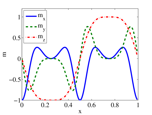
Figure 1: (Color online) The initial data for the magnetization equation (1). This initialization is obtained by allowing the orientation angles of the magnetization vector to vary sinusoidally in space, as in Eq. (8). Here the wave number of the variation is equal to the fundamental wave number $2\pi/L$.

the azimuthal angle $\theta\left(\bm{x},t\right)$, and the polar angle $\phi\left(\bm{x},t\right)$, where

$$m_{x}=|\bm{m}|\cos\phi\sin\theta,\qquad m_{y}=|\bm{m}|\sin\phi\sin\theta,\qquad m_{z}=|\bm{m}|\cos\theta,$$ (7)

and where $\phi\in\left[0,2\pi\right)$, and $\theta\in\left[0,\pi\right]$.

We carry out numerical simulations of Eqs. (1) and (3) on a periodic domain $\left[0,L\right]$, and outline the findings in what follows. Motivated by the change of coordinates (7), we choose the initial data

$$\phi_{0}\left(x\right)=\pi\left(1+\sin\left(2r\pi x/L\right)\right),\qquad\theta_{0}\left(x\right)=\tfrac{1}{2}\pi\left(1+\sin\left(2\pi sx/L\right)\right),$$ (8)

where $r$ and $s$ are integers. These data are shown in Fig. 1.

Case 1: Numerical simulations of Eq. (3). Equation (3) is usually solved by explicit or implicit finite differences Weinan2000 . We solve the equation by these methods, and by the explicit spectral method Zhu_numerics . The accuracy and computational cost is roughly the same in each case, and for simplicity, we therefore employ explicit finite differences; it is this method we use throughout the paper. Given the initial conditions (8), each component of the magnetization $\bm{m}=\left(m_{x},m_{y},m_{z}\right)$ tends to a constant, the energy

$$E=\tfrac{1}{2}\int_{\Omega}{dx}\left|\frac{\partial\bm{m}}{\partial{x}}\right|^{2}$$

decays with time, and $\left|\bm{m}\right|^{2}$ retains its initial value $|\bm{m}|^{2}=1$. After some transience, the decay of the energy functional becomes exponential in time. These results are shown in Fig. 2

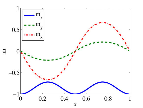
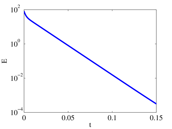
Figure 2: (Color online) Numerical simulations of Case (1), the Landau–Lifshitz–Gilbert equation in the over-damped limit. In this case, the magnetization decays to a constant state. Subfigures (a) and (b) show the magnetization at times $t=0.03$ and $t=0.15$ respectively; (c) is the energy functional, which exhibits exponential decay after some transience. The final orientation is $\left(\phi,\theta\right)=\left(\pi,\pi/2\right)$.

Case 2: Numerical simulations of Eq. (1) with $\alpha<\beta$. Given the smooth initial data (8), in time each component of the magnetization $\bm{m}=\left(m_{x},m_{y},m_{z}\right)$ decays to zero, while the energy

$$E=\tfrac{1}{2}\int_{\Omega}{dx}\bm{m}\cdot\left(1-\alpha^{2}\partial_{x}^{2}\right)^{-1}\bm{m}$$

tends to a constant value. Given our choice of initial conditions, the energy in fact increases to attain this constant value. Again the quantity $\left|\bm{m}\right|^{2}$ stays constant. These results are shown in Fig. 3. We find similar results when we set $\alpha=0$.

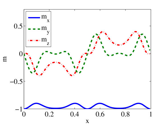
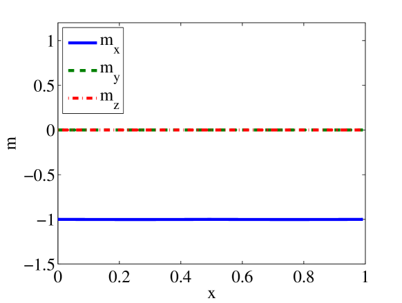
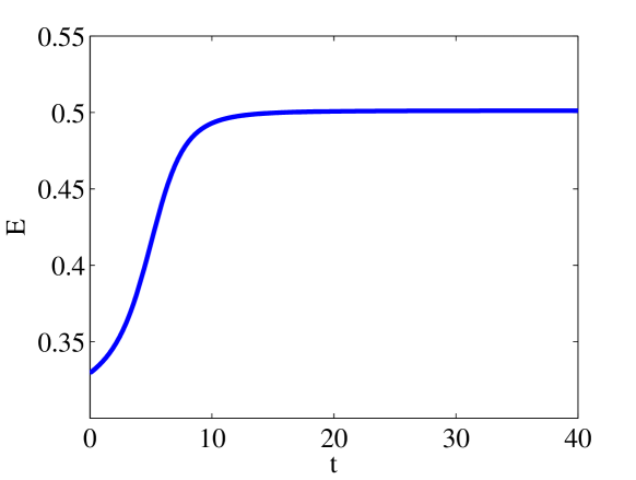
Figure 3: (Color online) Numerical simulations of Case (2), the non-local Gilbert equation with with $\alpha<\beta$. In this case, the energy increases to a constant value, and the magnetization becomes constant. Subfigures (a) and (b) show the magnetization at times $t=8$ and $t=40$; (c) is the energy functional. The final orientation is $\left(\phi,\theta\right)=\left(\pi,\pi/2\right)$.

Case 3: Numerical simulations of Eq. (1) with $\alpha>\beta$. Given the smooth initial data (8), in time each component of the magnetization $\bm{m}=\left(m_{x},m_{y},m_{z}\right)$ develops finer and finer scales. The development of small scales is driven by the decreasing nature of the energy functional, which decreases as power law at late times, and is reflected in snapshots of the power spectrum of the magnetization vector, shown in Fig. 4. As the system evolves, there

Case	Length scales	Energy	Outcome as $t\rightarrow\infty$	Linear Stability
(1)	$\beta=0$, $\delta{E}/\delta{\bm{m}}=-\partial_{x}^{2}\bm{m}$	Decreasing	Constant state	Stable
(2)	$\alpha<\beta$	Increasing	Constant state	Stable
(3)	$\alpha>\beta$	Decreasing	Development of finer and finer scales	Unstable

Table 1: Summary of the forms of Eq. (1) studied.

is a transfer of large amplitudes to higher wave numbers. This transfer slows down at late times, suggesting that the rate at which the solution roughens tends to zero, as $t\rightarrow\infty$. The evolution preserves the symmetry of the magnetization vector $\bm{m}\left(x,t\right)$ under parity transformations. This is seen by comparing Figs. 1 and 4. The energy is a decaying function of time, while the quantity $\left|\bm{m}\right|^{2}$ stays constant. We find similar results for the case when $\beta=0$.

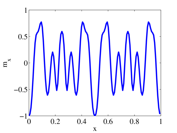
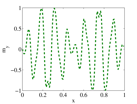
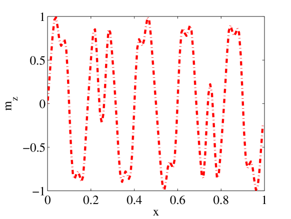
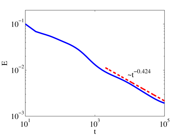
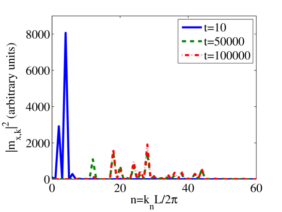
Figure 4: (Color online) Numerical simulations of Case (3), the non-local Gilbert equation with $\alpha>\beta$. In this case, the energy decreases indefinitely, and the magnetization vector develops finer and finer scales. Subfigures (a), (b), and (c) show the magnetization at time $t=10000$; (d) is the energy functional, which decreases in time as a power law at late times. Subfigure (e) shows the power spectrum of $m_{x}$; the integer index $n$ labels the spatial scales: if $k_{n}$ is a wavenumber, then the corresponding integer label is $n=k_{n}L/2\pi$.

These results can be explained qualitatively as follows. In Case (1), the energy functional exacts a penalty for the formation of gradients. The energy decreases with time and the the system evolves into a state in which no magnetization gradients are present, that is, a constant state. On the other hand, we have demonstrated that in Case (2), when $\alpha<\beta$, the energy increases to a constant value. Since in the non-local model, the energy functional represents the cost of forming smooth spatial structures, an increase in energy produces a smoother magnetization field, a process that continues until the magnetization reaches a constant value. Finally, in Case (3), when $\alpha>\beta$, the energy functional decreases, and this decrease corresponds to a roughening of the magnetization field, as seen in Fig. 4. In Sec. III we shall show that Case (2) is stable to small perturbations around a constant state, while Case (3) is unstable. Furthermore, we note that Case (2) and Case (3) differ only by a minus sign in Eq. (1), and are therefore related by time reversal. These results are summarized in Table 1.

The solutions of Eqs. (1) and (3) do not become singular. This is not surprising: the manifest conservation of $\left|\bm{m}\right|^{2}$ in Eqs. (1) and (3) provides a pointwise bound on the magnitude of the solution, preventing blow-up. Any addition to Eq. (1) that breaks this conservation law gives rise to the possibility of singular solutions, and it is to this possility that we now turn.

III Coupled density-magnetization equations

In this section we study a coupled density-magnetization equation pair that admit singular solutions. We investigate the linear stability of the equations and examine the conditions for instability. We find that the stability or otherwise of a constant state is controlled by the magnetization and density values of that state, and by the relative magnitude of the problem length scales. Using numerical and analytical techniques, we investigate the emergence and self-interaction of singular solutions.

The equations we study are as follows,

$$\frac{\partial\rho}{\partial t}=\frac{\partial}{\partial{x}}\left[\rho\left(\mu_{\rho}\frac{\partial}{\partial{x}}\frac{\delta{E}}{\delta\rho}+\bm{\mu}_{m}\cdot\frac{\partial}{\partial{x}}\frac{\delta{E}}{\delta\bm{m}}\right)\right],$$ (9a)

$$\frac{\partial\bm{m}}{\partial t}=\frac{\partial}{\partial x}\left[\bm{m}\left(\mu_{\rho}\frac{\partial}{\partial{x}}\frac{\delta{E}}{\delta\rho}+\bm{\mu}_{m}\cdot\frac{\partial}{\partial{x}}\frac{\delta{E}}{\delta\bm{m}}\right)\right]+\bm{m}\times\left(\bm{\mu}_{\bm{m}}\times\frac{\delta{E}}{\delta\bm{m}}\right),$$ (9b)

where we set

$$\mu_{\rho}=1,\qquad\frac{\partial{E}}{\partial\rho}=-\left(1-\alpha_{\rho}^{2}\partial_{x}^{2}\right)^{-1}\rho,$$

and, as before,

$$\bm{\mu}_{m}=\left(1-\beta_{m}^{2}\partial_{x}^{2}\right)^{-1}\bm{m},\qquad\frac{\delta E}{\delta\bm{m}}=\left(1-\alpha_{m}^{2}\partial_{x}^{2}\right)^{-1}\bm{m}.$$

These equations have been introduced by Holm, Putkaradze and Tronci in Darryl_eqn1 , using a kinetic-theory description. The density and the magnetization vector are driven by the velocity

$$V=\mu_{\rho}\frac{\partial}{\partial{x}}\frac{\delta{E}}{\delta\rho}+\bm{\mu}_{m}\cdot\frac{\partial}{\partial{x}}\frac{\delta{E}}{\delta\bm{m}}.$$ (10)

The velocity advects the ratio $|\bm{m}|/\rho$ by

$$\left(\frac{\partial}{\partial{t}}-V\frac{\partial}{\partial{x}}\right)\frac{|\bm{m}|}{\rho}=0.$$

We have the system energy

$$E=\tfrac{1}{2}\int_{\Omega}{dx}\bm{m}\cdot\left(1-\alpha_{m}^{2}\partial_{x}^{2}\right)^{-1}\bm{m}-\tfrac{1}{2}\int_{\Omega}{dx}\rho\left(1-\alpha_{\rho}^{2}\partial_{x}^{2}\right)^{-1}\rho,$$ (11)

and, given a non-negative density, the second term is always non-positive. This represents an energy of attraction, and we therefore expect singularities in the magnetization vector to arise from a collapse of the particle density due to the ever-decreasing energy of attraction. There are three length scales in the problem that control the time evolution: the ranges $\alpha_{m}$ and $\alpha_{\rho}$ of the potentials in Eq. (11), and the smoothening length $\beta_{m}$.

Linear stability analysis

We study the linear stability of the constant state $\left(\bm{m},\rho\right)=\left(\bm{m}_{0},\rho_{0}\right)$. We evaluate the smoothened values of this constant solution as follows,

$$\left(1-\alpha_{\rho}^{2}\partial_{x}^{2}\right)^{-1}\rho_{0} = f\left(x\right),$$

$$\rho_{0} = f\left(x\right)-\alpha_{\rho}^{2}\frac{d^{2}f}{dx^{2}},$$

$$f\left(x\right) = \rho_{0}+A\sinh\left(x/\alpha_{\rho}\right)+B\cosh\left(x/\alpha_{\rho}\right).$$

For periodic or infinite boundary conditions, the constants $A$ and $B$ are in fact zero and thus

$$\left(1-\alpha_{\rho}\partial_{x}^{2}\right)^{-1}\rho_{0}=\rho_{0},$$ (12)

and similarly $\bm{\mu}_{0}=\left(\delta E/\delta\bm{m}\right)_{\bm{m}_{0}}=\bm{m}_{0}$. The result (12) guarantees that the constant state $\left(\bm{m}_{0},\rho_{0}\right)$ is indeed a solution of Eq. (9b).

We study a solution $\left(\bm{m},\rho\right)=\left(\bm{m}_{0}+\delta\bm{m},\rho_{0}+\delta\rho\right)$, which represents a perturbation away from the constant state. By assuming that $\delta\bm{m}$ and $\delta\rho$ are initially small in magnitude, we obtain the following linearized equations for the perturbation density and magnetization,

$$\frac{\partial}{\partial t}\delta\rho=-\rho_{0}\frac{\partial^{2}}{\partial{x}^{2}}\left(1-\alpha_{\rho}^{2}\partial_{x}^{2}\right)^{-1}\delta\rho+\rho_{0}\frac{\partial^{2}}{\partial{x}^{2}}\left(1-\alpha_{m}^{2}\partial_{x}^{2}\right)^{-1}\bm{m}_{0}\cdot\delta\bm{m},$$ (13)

$$\frac{\partial}{\partial t}\delta\bm{m}=\bm{m}_{0}\left[-\frac{\partial^{2}}{\partial{x}^{2}}\left(1-\alpha_{\rho}^{2}\partial_{x}^{2}\right)^{-1}\delta\rho+\frac{\partial^{2}}{\partial{x}^{2}}\left(1-\alpha_{m}^{2}\partial_{x}^{2}\right)^{-1}\bm{m}_{0}\cdot\delta\bm{m}\right]\\ +\bm{m}_{0}\times\Big{\{}\bm{m}_{0}\times\left[\left(1-\alpha_{m}^{2}\partial_{x}^{2}\right)^{-1}\delta\bm{m}-\left(1-\beta_{m}^{2}\partial_{x}^{2}\right)^{-1}\delta\bm{m}\right]\Big{\}}.$$

For $\bm{m}_{0}\neq 0$ we may choose two unit vectors $\hat{\bm{n}}_{1}$ and $\hat{\bm{n}}_{2}$ such that $\bm{m}_{0}/|\bm{m}_{0}|$, $\hat{\bm{n}}_{1}$ and $\hat{\bm{n}}_{2}$ form an orthonormal triad (that is, we have effected a change of basis). We then study the quantities $\delta\rho$, $\delta\chi$, $\delta\xi_{1}$ and $\delta\xi_{2}$, where

$$\delta\chi=\bm{m}_{0}\cdot\delta\bm{m},\qquad\delta\xi_{1}=\hat{\bm{n}}_{1}\cdot\delta\bm{m},\qquad\delta\xi_{2}=\hat{\bm{n}}_{2}\cdot\delta\bm{m}.$$

We obtain the linear equations

$$\frac{\partial}{\partial t}\delta\rho=-\rho_{0}\frac{\partial^{2}}{\partial{x}^{2}}\left(1-\alpha_{\rho}^{2}\partial_{x}^{2}\right)^{-1}\delta\rho+\rho_{0}\frac{\partial^{2}}{\partial{x}^{2}}\left(1-\alpha_{m}^{2}\partial_{x}^{2}\right)^{-1}\delta\chi,$$

$$\frac{\partial}{\partial t}\delta\chi=-|\bm{m}_{0}|^{2}\frac{\partial^{2}}{\partial{x}^{2}}\left(1-\alpha_{\rho}^{2}\partial_{x}^{2}\right)^{-1}\delta\rho+|\bm{m}_{0}|^{2}\frac{\partial^{2}}{\partial{x}^{2}}\left(1-\alpha_{m}^{2}\partial_{x}^{2}\right)^{-1}\delta\chi,$$

$$\frac{\partial}{\partial t}\delta\xi_{i}=\left[\left(1-\beta_{m}^{2}\partial_{x}^{2}\right)^{-1}-\left(1-\alpha_{m}^{2}\partial_{x}^{2}\right)^{-1}\right]\delta\xi_{i},\qquad i=1,2.$$

By focusing on a single-mode disturbance with wave number $k$ we obtain the following system of equations

$$\frac{d}{dt}\left(\begin{array}[]{c}\delta\rho\\ \delta\chi\\ \delta\xi_{1}\\ \delta\xi_{2}\end{array}\right)=\left(\begin{array}[]{cccc}\frac{\rho_{0}k^{2}}{1+\alpha_{\rho}^{2}k^{2}}&-\frac{\rho_{0}k^{2}}{1+\alpha_{m}^{2}k^{2}}&0&0\\ \frac{|\bm{m}_{0}|^{2}k^{2}}{1+\alpha_{\rho}^{2}k^{2}}&-\frac{|\bm{m}_{0}|^{2}k^{2}}{1+\alpha_{m}^{2}k^{2}}&0&0\\ 0&0&\frac{1}{1+\beta_{m}^{2}k^{2}}-\frac{1}{1+\alpha_{m}^{2}k^{2}}&0\\ 0&0&0&\frac{1}{1+\beta_{m}^{2}k^{2}}-\frac{1}{1+\alpha_{m}^{2}k^{2}}\end{array}\right)\left(\begin{array}[]{c}\delta\rho\\ \delta\chi\\ \delta\xi_{1}\\ \delta\xi_{2}\end{array}\right),$$

with eigenvalues

$$\sigma_{0}=0,\qquad\sigma_{1}=\frac{\rho_{0}k^{2}}{1+\alpha_{\rho}^{2}k^{2}}-\frac{|\bm{m}_{0}|^{2}k^{2}}{1+\alpha_{m}^{2}k^{2}},\qquad\sigma_{2}=\frac{1}{1+\beta_{m}^{2}k^{2}}-\frac{1}{1+\alpha_{m}^{2}k^{2}}.$$ (14)

The eigenvalues are the growth rate of the disturbance $\left(\delta\rho,\delta\chi,\delta\xi_{1},\delta\xi_{2}\right)$ ChandraFluids . There are two routes to instability, when $\sigma_{1}>0$, or when $\sigma_{2}>0$. The first route leads to an instability when

$$\sigma_{1}>0,\qquad\frac{\rho_{0}}{|\bm{m}_{0}|^{2}}>\frac{1+\alpha_{\rho}^{2}k^{2}}{1+\alpha_{m}^{2}k^{2}},$$

while the second route leads to instability when

$$\sigma_{2}>0,\qquad\alpha_{m}>\beta_{m}.$$

We have plotted the growth rates for the case when $\rho_{0}=|\bm{m}_{0}|^{2}=1$, and compared the theory with numerical simulations. There is excellent agreement at low wave numbers, although the numerical simulations become less accurate at high wave numbers. This can be remedied by increasing the resolution of the simulations. These plots are shown in Figs. 5 and 6.

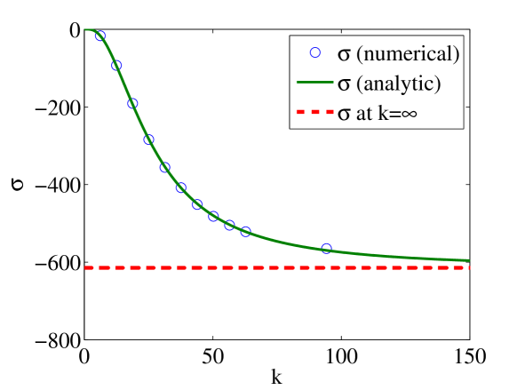
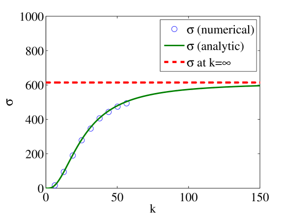
Figure 5: (Color online) The first route to instability. Subfigure (a) shows the growth rate $\sigma_{1}$ for $\alpha_{m}<\beta_{m}<\alpha_{\rho}$, with negativity indicating a stable equilibrium; (b) gives the growth rate $\sigma_{1}$ for $\alpha_{\rho}<\alpha_{m}<\beta_{m}$, with positivity indicating an unstable equilibrium. We have set $|\bm{m}_{0}|=\rho_{0}=1$.

The growth rates $\sigma_{1,2}$ are parabolic in $k$ at small $k$; $\sigma_{1}$ saturates at large $k$, while $\sigma_{2}$ attains a maximum and decays at large $k$. The growth rates can be positive or negative, depending on the initial configuration, and on the relationship between the problem length scales. In contrast to some standard instabilities of pattern formation (e.g. Cahn–Hilliard Argentina2005 or Swift–Hohenberg OjalvoBook ), the $\sigma_{1}$-unstable state becomes more unstable at higher wave numbers (smaller scales), thus preventing the ‘freezing-out’ of the instability by a reduction of the box size Argentina2005 . The growth at small scales is limited,

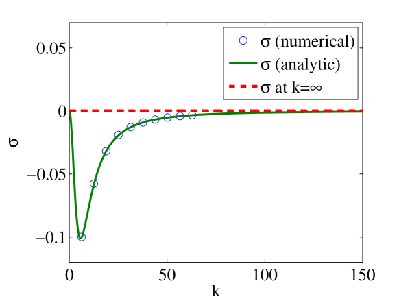
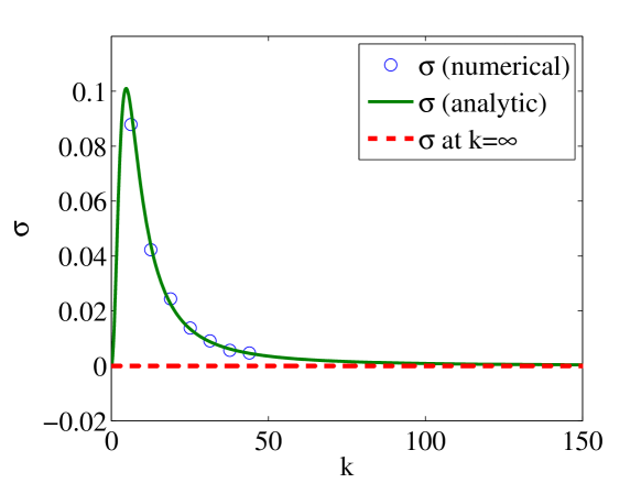
Figure 6: (Color online) The second route to instability. Subfigure (a) shows the growth rate $\sigma_{2}$ for $\alpha_{m}<\beta_{m}$, with negativity indicating a stable equilibrium; (b) gives the growth rate $\sigma_{2}$ for $\alpha_{m}>\beta_{m}$, with positivity indicating an unstable equilibrium. We have set $|\bm{m}_{0}|=\rho_{0}=1$.

however, by the saturation in $\sigma$ as $k\rightarrow\infty$. Heuristically, this can be explained as follows: at higher wave number, the disturbance $\left(\delta\rho,\delta\chi,\delta\xi_{1},\delta\xi_{2}\right)$ gives rise to more and more peaks per unit length. This makes merging events increasingly likely, so that peaks combine to form larger peaks, enhancing the growth of the disturbance.

Recall in Sec. II that the different behaviors of the magnetization equation (1) are the result of a competition between the length scales $\alpha_{m}$ and $\beta_{m}$. For $\alpha_{m}<\beta_{m}$ the initial (large-amplitude) disturbance tends to a constant, while for $\alpha_{m}>\beta_{m}$ the initial disturbance develops finer and finer scales. In this section, we have shown that the coupled density-magnetization equations are linearly stable when $\alpha_{m}<\beta_{m}$, while the reverse case is unstable. In contrast to the first route to instability, the growth rate $\sigma_{2}$, if positive, admits a maximum. This is obtained by setting $\sigma_{2}^{\prime}\left(k\right)=0$. Then the maximum growth rate occurs at a scale

$$\lambda_{\mathrm{max}}:=2\pi k_{\mathrm{max}}^{-1}=2\pi\sqrt{\alpha_{m}\beta_{m}}.$$

Thus, the scale at which the disturbance is most unstable is determined by the geometric mean of $\alpha_{m}$ and $\beta_{m}$. Given a disturbance $\left(\delta\rho,\delta\chi,\delta\xi_{1},\delta\xi_{2}\right)$ with a range of modes initially present, the instability selects the disturbance on the scale $\lambda_{\mathrm{max}}$. This disturbance develops a large amplitude and a singular solution subsequently emerges. It is to this aspect of the problem that we now turn.

Singular solutions

In this section we show that a finite weighted sum of delta functions satisfies the partial differential equations (9b). Each delta function has the interpretation of a particle or clumpon, whose weights and positions satisfy a finite set of ordinary differential equations. We investigate the two-clumpon case analytically and show that the clumpons tend to a state in which they merge, diverge, or are separated by a fixed distance. In each case, we determine the final state of the clumpon magnetization.

To verify that singular solutions are possible, let us substitute the ansatz

$$\rho\left(x,t\right)=\sum_{i=1}^{M}a_{i}\left(t\right)\delta\left(x-x_{i}\left(t\right)\right),\qquad\bm{m}\left(x,t\right)=\sum_{i=1}^{M}\bm{b}_{i}\left(t\right)\delta\left(x-x_{i}\left(t\right)\right),$$ (15)

into the weak form of equations (9b). Here we sum over the different components of the singular solution (which we call clumpons). In this section we work on the infinite domain $x\in\left(-\infty,\infty\right)$. The weak form of the equations is obtained by testing Eqs. (9b) with once-differentiable functions $\phi\left(x\right)$ and $\bm{\psi}\left(x\right)$,

$$\frac{d}{dt}\int_{-\infty}^{\infty}{dx}\rho\left(x,t\right)\phi\left(x\right)=-\int_{-\infty}^{\infty}{dx}\phi^{\prime}\left(x,t\right)\left(\mu_{\rho}\frac{\partial}{\partial{x}}\frac{\delta{E}}{\delta\rho}+\bm{\mu}_{\bm{m}}\cdot\frac{\partial}{\partial{x}}\frac{\delta{E}}{\delta\bm{m}}\right),$$ (16a)

$$\frac{d}{dt}\int_{-\infty}^{\infty}{dx}\bm{m}\left(x,t\right)\cdot\bm{\psi}\left(x\right)=-\int_{-\infty}^{\infty}{dx}\bm{\psi}^{\prime}\left(x\right)\cdot\bm{m}\left(x,t\right)\left(\mu_{\rho}\frac{\partial}{\partial{x}}\frac{\delta{E}}{\delta\rho}+\bm{\mu}_{\bm{m}}\cdot\frac{\partial}{\partial{x}}\frac{\delta{E}}{\delta\bm{m}}\right)\\ +\int_{-\infty}^{\infty}{dx}\bm{\psi}\left(x\right)\cdot\left[\bm{m}\times\left(\bm{\mu}_{\bm{m}}\times\frac{\delta{E}}{\delta\bm{m}}\right)\right],$$ (16b)

Substitution of the ansatz (15) into the weak equations (16b) yields the relations

$$\frac{da_{i}}{dt}=0,\qquad\frac{dx_{i}}{dt}=-V\left(x_{i}\right),\qquad\frac{d\bm{b}_{i}}{dt}=\bm{b}_{i}\times\left(\bm{\mu}\times\frac{\delta{E}}{\delta\bm{m}}\right)\left(x_{i}\right),\qquad i\in\{1,...,M\},$$ (17)

where $V$ and $\left(\bm{\mu}\times\left({\delta{E}}/{\delta\bm{m}}\right)\right)$ are obtained from the ansatz (15) and are evaluated at $x_{i}$. Note that the density weights $a_{i}$ and the magnitude of the weights $\bm{b}_{i}$ remain constant in time.

We develop further understanding of the clumpon dynamics by studying the two-clumpon version of Eqs. (17). Since the weights $a_{1}$, $a_{2}$, $|\bm{b}_{1}|$, and $|\bm{b}_{2}|$ are constant, two variables suffice to describe the interaction: the relative separation $x=x_{1}-x_{2}$ of the clumpons, and the cosine of the angle between the clumpon magnetizations, $\cos\varphi=\bm{b}_{1}\cdot\bm{b}_{2}/|\bm{b}_{1}||\bm{b}_{2}|$. Using the properties of the kernel $H\left(0\right)=1$, $H^{\prime}\left(0\right)=0$, we derive the equations

$$\frac{dx}{dt}=MH_{\alpha_{\rho}}^{\prime}\left(x\right)-B_{1}H^{\prime}_{\alpha_{m}}\left(x\right)H_{\beta_{m}}\left(x\right)-B_{2}H_{\alpha_{m}}^{\prime}\left(x\right)y,\qquad y=\cos\varphi$$ (18a)

$$\frac{dy}{dt}=B_{2}\left(1-y^{2}\right)\left[H_{\beta_{m}}\left(x\right)-H_{\alpha_{m}}\left(x\right)\right],$$ (18b)

where $M=a_{1}+a_{2}$, $B_{1}=|\bm{b}_{1}|^{2}+|\bm{b}_{2}|^{2}$, and $B_{2}=2|\bm{b}_{1}||\bm{b}_{2}|$ are constants. Equations (18b) form a dynamical system whose properties we now investigate using phase-plane analysis StrogatzBook . We note first

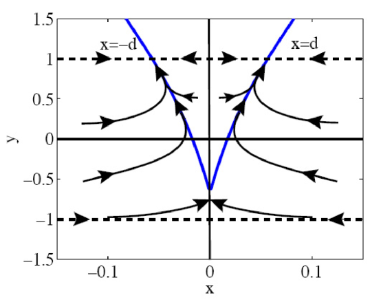
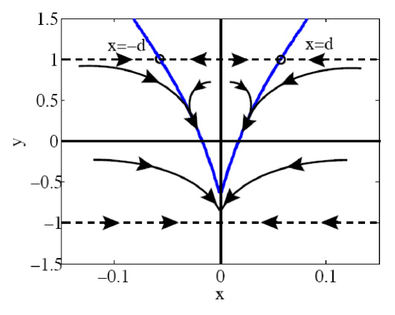
Figure 7: (Color online) The nullcline $dx/dt=0$ of the two-clumpon dynamical system with $\alpha_{m}<\alpha_{\rho}$. The region contained inside the dotted lines $y=\pm 1$ gives the allowed values of the dynamical variables $\left(x,y\right)$. Subfigure (a) shows the case when $\beta_{m}<\alpha_{m}$. The stable equilibria of the system are $\left(x,y\right)=\left(\pm{d},1\right)$ and the line $x=0$. All initial conditions flow into one of these equilibrium states; subfigure (b) shows the case when $\alpha_{m}<\beta_{m}$. Initial conditions confined to the line $y=1$ flow into the fixed point $\left(\pm{d},1\right)$, while all other initial conditions flow into the line $x=0$.

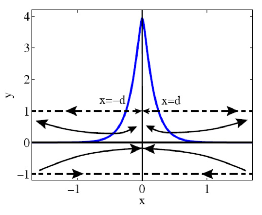
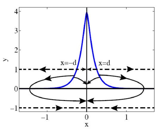
Figure 8: (Color online) The nullcline $dx/dt=0$ of the two-clumpon dynamical system with $\alpha_{\rho}<\alpha_{m}$. The region contained inside the dotted lines $y=\pm 1$ gives the allowed values of the dynamical variables $\left(x,y\right)$. Subfigure (a) shows the case when $\beta_{m}<\alpha_{m}$. The lines $x=0$ and $x=\pm\infty$ form the stable equilibria of the system. All initial conditions flow into one of these states; subfigure (b) shows the case when $\alpha_{m}<\beta_{m}$. Initial conditions confined to the line $y=1$ flow into the fixed points $\left(0,1\right)$ and $\left(\pm\infty,1\right)$, while all other initial conditions flow into the line $x=0$.

of all that the $|y|>1$ region of the phase plane is forbidden, since the $y$-component of the vector field $\left(dx/dt,dy/dt\right)$ vanishes at $|y|=1$. The vertical lines $x=0$ and $x=\pm\infty$ are equilibria, although their stability will depend on the value of the parameters $\left(\alpha_{m},\alpha_{\rho},\beta_{m},B_{1},B_{2},M\right)$. The curve across which $dx/dt$ changes sign is called the nullcline. This is given by

$$y=\frac{MH_{\alpha_{\rho}}^{\prime}\left(x\right)-B_{1}H^{\prime}_{\alpha_{m}}\left(x\right)H_{\beta_{m}}\left(x\right)}{B_{2}H^{\prime}_{\alpha_{m}}\left(x\right)},$$

which on the domain $x\in\left(-\infty,\infty\right)$ takes the form

$$y=\frac{\alpha_{m}}{B_{2}}\left[\frac{M}{\alpha_{\rho}}e^{-|x|\left(\frac{1}{\alpha_{\rho}}-\frac{1}{\alpha_{m}}\right)}-\frac{B_{1}}{\alpha_{m}}e^{-\frac{1}{\beta_{m}}|x|}\right].$$

Several qualitatively different behaviors are possible, depending on the magnitude of the values taken by the parameters $\left(\alpha_{m},\alpha_{\rho},\beta_{m},B_{1},B_{2},M\right)$. Here we outline four of these behavior types.

• Case 1: The length scales are in the relation $\alpha_{m}<\alpha_{\rho}$, and $\beta_{m}<\alpha_{m}$. The vector field $\left(dx/dt,dy/dt\right)$ and the nullcline are shown in Fig. 7 (a). There is flow into the fixed points $\left(x,y\right)=\left(\pm{d},1\right)$, and into the line $x=0$, while $y$ is a non-decreasing function of time, which follows from Eq. (18b). The ultimate state of the system is thus $x=\pm{d}$, $\varphi=0$ (alignment), or $x=0$ (merging). In the latter case the final orientation is given by the integral of Eq. (18b),

  $$\tan\left(\frac{\varphi}{2}\right)=\tan\left(\frac{\varphi_{0}}{2}\right)\exp\left[-B_{2}\int_{0}^{\infty}{dt}\left[H_{\beta_{m}}\left(x\left(t\right)\right)-H_{\alpha_{m}}\left(x\left(t\right)\right)\right]\right],\qquad\varphi_{0}=\varphi\left(t=0\right).$$ (19)

• Case 2: The length scales are in the relation $\alpha_{m}<\alpha_{\rho}$, $\alpha_{m}<\beta_{m}$. The vector field and the nullcline are shown in Fig. 7 (b). All flow not confined to the line $y=1$ is into the line $x=0$, since $y$ is now a non-increasing function of time. The ultimate state of the system is thus $x=\pm{d}$, $\varphi=0$ (alignment), or $x=0$ (merging). In the latter case the final orientation is given by the formula (19).

• Case 3: The length scales are in the relation $\alpha_{\rho}<\alpha_{m}$ and $\beta_{m}<\alpha_{m}$. The vector field and the nullcline are shown in Fig. 8 (a). Inside the region bounded by the line $y=0$ and the nullcline, the flow is into the line $x=0$ (merging), and the fixed points $\left(\pm{d},1\right)$ are unstable. The flow below the line $y=0$ is towards the line $x=0$. Outside of these regions, however, the flow is into the lines $x=\pm\infty$, which shows that for a suitable choice of parameters and initial conditions, the clumpons can be made to diverge.

• Case 4: The length scales are in the relation $\alpha_{\rho}<\alpha_{m}$ and $\alpha_{m}<\beta_{m}$. The vector field and the nullcline are shown in Fig. 8 (b). The quantity $y$ is a non-increasing function of time. All flow along the line $y=1$ is directed away from the fixed points $\left(\pm{d},1\right)$ and is into the fixed points $\left(0,1\right)$, or $\left(\pm\infty,1\right)$. All other initial conditions flow into $x=0$, although initial conditions that start above the curve formed by the nullcline flow in an arc and eventually reach a fixed point $\left(x=0,y<0\right)$.

We summarize the cases we have discussed in Table 2. Using numerical simulations of Eqs. (18b), we have verified that Cases (1)–(4) do indeed occur. The list of cases we have considered is not exhaustive: depending on the parameters $B_{1}$, $B_{2}$, and $M$, other phase portraits may arise. Indeed, it is clear from Fig. 7 that through saddle-node bifurcations, the fixed points $\left(x,y\right)=\left(\pm{d},1\right)$ may disappear, or additional fixed points $\left(x,y\right)=\left(\pm{d^{\prime}},-1\right)$ may appear. Our

Case	$\alpha_{m}$ vs. $\alpha_{\rho}$	$\alpha_{m}$ vs. $\beta_{m}$	Equilibria	Flow
(1)	$\alpha_{m}<\alpha_{\rho}$	$\beta_{m}<\alpha_{m}$	$\left(x,y\right)=\left(\pm{d},1\right)$; $x=0$; $x=\pm\infty$	Flow into $x=0$ and $\left(x,y\right)=\left(\pm{d},1\right)$
(2)	$\alpha_{m}<\alpha_{\rho}$	$\alpha_{m}<\beta_{m}$	$\left(x,y\right)=\left(\pm{d},1\right)$; $x=0$; $x=\pm\infty$	Flow into $x=0$ and $\left(x,y\right)=\left(\pm{d},1\right)$
(3)	$\alpha_{\rho}<\alpha_{m}$	$\beta_{m}<\alpha_{m}$	$\left(x,y\right)=\left(\pm{d},1\right)$; $x=0$; $x=\pm\infty$	Flow into $x=0$ and $x=\pm\infty$
(4)	$\alpha_{\rho}<\alpha_{m}$	$\alpha_{m}<\beta_{m}$	$\left(x,y\right)=\left(\pm{d},1\right)$; $x=0$; $x=\pm\infty$	Flow into $x=0$ and $x=\pm\infty$

Table 2: Summary of the distinct phase portraits of Eq. (18b) studied.

analysis shows, however, that it is possible to choose a set of parameters $\left(\alpha_{\rho},\alpha_{m},\beta_{m},B_{1},B_{2},M\right)$ such that two clumpons either merge, diverge, or are separated by a fixed distance.

Numerical Simulations

To examine the emergence and subsequent interaction of the clumpons, we carry out numerical simulations of Eq. (9b) for a variety of initial conditions. We use an explicit finite-difference algorithm with a small amount of artifical diffusion. We solve the following weak form of Eq. (9b), obtained by testing Eq. (16b) with $H_{\beta_{m}}$,

$$\frac{\partial\overline{\rho}}{\partial{t}}=D_{\mathrm{artif}}\frac{\partial^{2}\overline{\rho}}{\partial{x^{2}}}+\int_{\Omega}{dy}H_{\beta_{m}}^{\prime}\left(x-y\right)\rho\left(y,t\right)V\left(y,t\right),$$

$$\frac{\partial\mu_{i}}{\partial{t}}=D_{\mathrm{artif}}\frac{\partial^{2}\mu_{i}}{\partial{x^{2}}}+\int_{\Omega}{dy}H_{\beta_{m}}^{\prime}\left(x-y\right)\bm{m}_{i}\left(y,t\right)V\left(y,t\right)\\ +\int_{\Omega}{dy}H_{\beta_{m}}\left(x-y\right)\bm{e}_{i}\cdot\left[\bm{m}\times\left(\bm{\mu}\times\frac{\delta{E}}{\delta\bm{m}}\right)\right],$$

where $\overline{\rho}=H_{\beta_{m}}*\rho$ and $\bm{e}_{i}$ is the unit vector in the $i^{\mathrm{th}}$ direction. We work on a periodic domain $\Omega=\left[-L/2,L/2\right]$, at a resolution of $250$ gridpoints; going to higher resolution does not noticeably increase the accuracy of the results.

The first set of initial conditions we study is the following,

$$\bm{m}\left(x,0\right) = \left(\sin\left(4k_{0}x+\phi_{x}\right),\sin\left(4k_{0}x+\phi_{y}\right),\sin\left(4k_{0}x+\phi_{z}\right)\right),$$

$$\rho\left(x,0\right) = 0.5+0.35\cos\left(2k_{0}x\right),$$ (20)

where $\phi_{x}$, $\phi_{y}$, and $\phi_{z}$ are random phases in the interval $\left[0,2\pi\right]$, and $k_{0}=2\pi/L$ is the fundamental wave number. The initial conditions for the magnetization vector are chosen to represent the lack of a preferred direction in the problem. The time evolution of equations (9b) for this set of initial conditions is shown in Fig. 9. After a short time, the initial data become singular, and subsequently, the solution $\left(\rho,\bm{m}\right)$ can be represented as a sum of clumpons,

$$\rho\left(x,t\right)=\sum_{i=1}^{M}a_{i}\delta\left(x-x_{i}\left(t\right)\right),\qquad\bm{m}\left(x,t\right)=\sum_{i=1}^{M}\bm{b}_{i}\left(t\right)\delta\left(x-x_{i}\left(t\right)\right),\qquad M=2.$$

Here $M=2$ is the number of clumpons present at the singularity time. This number corresponds to the number of maxima in the initial density profile. The forces exerted by each clumpon on the other balance because of the effect of the periodic boundary conditions. Indeed, any number of equally-spaced, identical, interacting particles arranged on a ring are in equilibrium, although this equilibrium is unstable for an attractive force. Thus, at late times, the clumpons are stationary, while the magnetization vector $\bm{\mu}$ shows alignment of clumpon magnetizations.

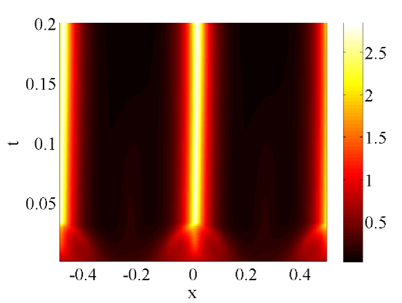
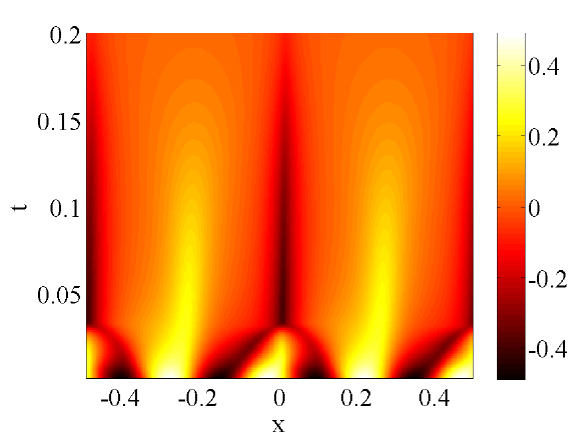
Figure 9: (Color online) Evolution of sinusoidally-varying initial conditions for the density and magnetization, as in Eq. (20). Subfigure (a) shows the evolution of $H_{\rho}*\rho$ for $t\in\left[0,0.15\right]$, by which time the initial data have formed two clumpons; (b) shows the evolution of $\mu_{x}$. The profiles of $\mu_{y}$ and $\mu_{z}$ are similar. Note that the peaks in the density profile correspond to the troughs in the magnetization profile. This agrees with the linear stability analysis, wherein disturbances in the density give rise to disturbances in the magnetization.

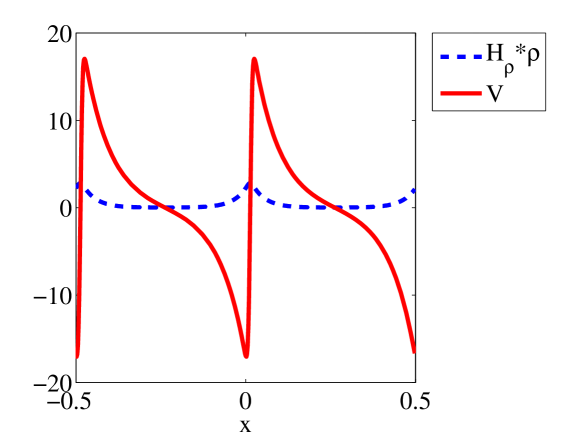
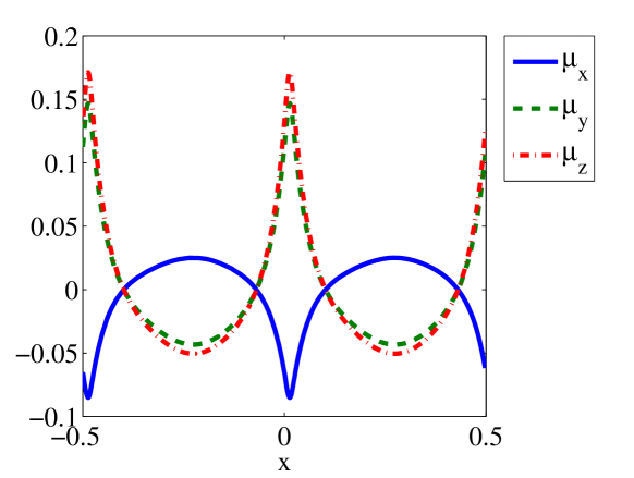
Figure 10: (Color online) Evolution of sinusoidally-varying initial conditions for the density and magnetization, as in Eq. (20). Subfigure (a) shows the system velocity $V$ given in Eq. (10), just before the singularity time; (b) shows the magnetization $\bm{\mu}$ at the same time. The density maxima emerge at the locations where the convergence of $-V$ (flow into $x=0$ and $x=\pm L/2$) occurs, and the magnetization develops extrema there.

We gain further understanding of the formation of singular solutions by studying the system velocity $V$ just before the onset of the singularity. This is done in Fig. 10. Figure 10 (a) shows the development of the two clumpons from the initial data. Across each density maximum, the velocity has the profile $V\approx\lambda\left(t\right)x$, where $\lambda\left(t\right)>0$ is an increasing function of time. This calls to mind the advection problem for the scalar $\theta\left(x,t\right)$, studied by Batchelor in the context of passive-scalar mixing Batchelor1959

$$\frac{\partial\theta}{\partial t}=\lambda_{0}x\frac{\partial\theta}{\partial{x}},\qquad\lambda_{0}>0.$$

Given initial data $\theta\left(x,0\right)=\theta_{0}e^{-x^{2}/\ell_{0}^{2}}$, the solution evolves in time as

$$\theta\left(x,t\right)=\theta_{0}e^{-x^{2}/\left(\ell_{0}^{2}e^{-2\lambda_{0}{t}}\right)},$$

so that gradients are amplified exponentially in time,

$$\frac{\partial\theta}{\partial{x}}=-\frac{2\theta_{0}}{\ell_{0}^{2}}xe^{\lambda_{0}{t}}e^{-x^{2}/\left(\ell_{0}^{2}e^{-2\lambda_{0}{t}}\right)},$$

in a similar manner to the problem studied.

The evolution of the set of initial conditions (20) has therefore demonstrated the following: the local velocity $V$ is such that before the onset of the singularity, matter is compressed into regions where $\rho\left(x,0\right)$ is large, to such an extent that the matter eventually accumulates at isolated points, and the singular solution emerges. Moreover, the density maxima, rather than the magnetization extrema, drive the formation of singularities. This is not surprising, given that the attractive part of the system’s energy comes from density variations.

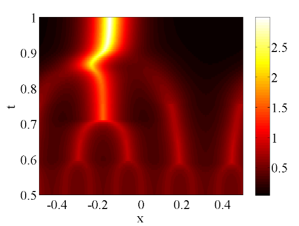
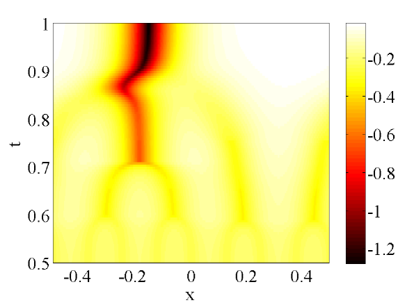
Figure 11: (Color online) Evolution of a flat magnetization field and a sinusoidally-varying density, as in Eq. (21). Subfigure (a) shows the evolution of $H_{\rho}*\rho$ for $t\in\left[0.5,1\right]$; (b) shows the evolution of $\mu_{x}$. The profiles of $\mu_{y}$ and $\mu_{z}$ are similar. At $t=0.5$, the initial data have formed eight equally spaced, identical clumpons, corresponding to the eight density maxima in the initial configuration. By impulsively shifting the clumpon at $x=0$ by a small amount, the equilibrium is disrupted and the clumpons merge repeatedly until only one clumpon remains.

To highlight the interaction between clumpons, we examine the following set of initial conditions,

$$\bm{m}\left(x,0\right)=\bm{m}_{0}=\text{const.},\qquad\rho\left(x,0\right)=0.5+0.35\cos\left(8k_{0}x\right),$$ (21)

where $k_{0}=2\pi/L$ is the fundamental wave number. Since this set of initial conditions contains a large number of density maxima, we expect a large number of closely-spaced clumpons to emerge, and this will illuminate the clumpon interactions. The time evolution of equations (9b) for this set of initial conditions is shown in Fig. 11. As before, the solution becomes singular after a short time, and is subsequently represented by a sum of clumpons,

$$\rho\left(x,t\right)=\sum_{i=1}^{M}a_{i}\delta\left(x-x_{i}\left(t\right)\right),\qquad\bm{m}\left(x,t\right)=\sum_{i=1}^{M}\bm{b}_{i}\left(t\right)\delta\left(x-x_{i}\left(t\right)\right),\qquad M=8.$$

Here $M=8$ is the number of clumpons at the singularity time. This number corresponds to the number of maxima in the initial density profile. As before, this configuration of equally spaced, identical clumpons is an equilibrium state, due to periodic boundary conditions. Therefore, once the particle-like state has formed, we impulsively shift the clumpon at $x=0$ by a small amount, and precipitate the merging of clumpons. The eight clumpons then merge repeatedly until only a single clumpon remains. The tendency for the clumpons to merge is explained by the velocity $V$, which changes sign across a clumpon. Thus, if a clumpon is within the range of the force exerted by its neighbours, the local velocity, if unbalanced, will advect a given clumpon

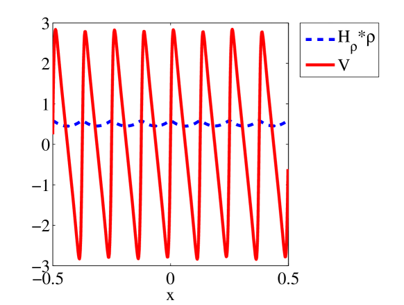
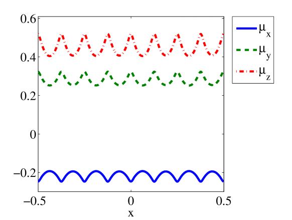
Figure 12: (Color online) Evolution of a flat magnetization field and a sinusoidally-varying density, as in Eq. (21). Subfigure (a) shows the system velocity $V$ given in Eq. (10) just before the singularity time; (b) gives the magnetization $\bm{\mu}$ at the same time. The density maxima emerge at the locations where the convergence of $-V$ occurs, and the magnetization develops extrema there.

in the direction of one of its neighbours, and the clumpons merge. This process is shown in Fig. 13.

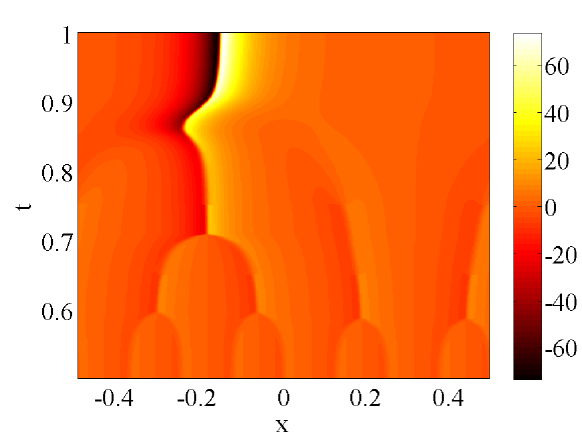
Figure 13: (Color online) Evolution of a flat magnetization field and a sinusoidally-varying density, as in Eq. (21). Shown is the velocity profile for $t\in\left[0.5,1\right]$; the system velocity is given by Eq. (10). The velocity $-V$ flows into each density maximum, concentrating matter at isolated points and precipitating the formation of eight equally-spaced identical clumpons. On a periodic domain, such an arrangement is an equilibrium state, although it is unstable. Thus, by impulsively shifting the clumpon at $x=0$ by a small amount, we force the clumpons to collapse into larger clumpons, until only a single clumpon remains.

IV Conclusions

We have investigated the non-local Gilbert (NG) equation introduced by Holm, Putkaradze, and Tronci in Darryl_eqn1 using a combination of numerical simulations and simple analytical arguments. The NG equation contains two competing length scales of non-locality: there is a length scale $\alpha$ associated with the range of the interaction potential, and a length scale $\beta$ that governs the smoothened magnetization vector that appears in the equation. When $\alpha<\beta$ all initial configurations of the magnetization tend to a constant value; while for $\beta<\alpha$ the initial configuration of the magnetization field develops finer and finer scales. These two effects are in balance when $\alpha=\beta$, and the system does not evolve away from its initial state. Furthermore, the NG equation conserves the norm of the magnetization vector $\bm{m}$, thus providing a pointwise bound on the solution and preventing the formation of singular solutions.

To study the formation of singular solutions, we couple the NG equation to a scalar density equation. Associated with the scalar density is a negative energy of attraction that drives the formation of singular solutions and breaks the pointwise bound on the $\bm{m}$. Three length scales of non-locality now enter into the problem: the range of the force associated with the scalar density, the range of the force due to the magnetization, and the smoothening length. As before, the competition of length scales is crucial to the evolution of the system; this is seen in the linear stability analysis of the coupled equations, in which the relative magnitude of the length scales determines the stability or otherwise of a constant state.

Using numerical simulations, we have demonstrated the emergence of singular solutions from smooth initial data, and have explained this behavior by the negative energy of attraction produced by the scalar density. The singular solution consists of a weighted sum of delta functions, given in Eq. (15), which we interpret as interacting particles or clumpons. The clumpons evolve under simple finite-dimensional dynamics. We have shown that a system of two clumpons is governed by a two-dimensional dynamical system that has a multiplicity of steady states. Depending on the length scales of non-locality and the clumpon weights, the two clumpons can merge, diverge, or align and remain separated by a fixed distance.

Our paper thus gives a qualitative description of the dynamics. Future work will focus on the regularity of solutions of the NG equation, and the existence and regularity of solutions for the coupled density-magnetization equations. Bertozzi and Laurent Bertozzi2007 have studied the simpler (uncoupled) non-local scalar density equation, proving existence, uniqueness, and blowup results using techniques from functional analysis, and a similar analysis will illuminate the equations we have studied. The behavior of singular solutions in higher dimensions is another topic that deserves further study.

DDH was partially supported by the US Department of Energy, Office of Science, Applied Mathematical Research and the Royal Society Wolfson Research Merit Award. CT was also partially supported by the Royal Society Wolfson Research Merit Award. L.Ó.N. was supported by the Irish government and the UK Engineering and Physical Sciences Research Council.

References

- (1) F. A. Denis, P. Hanarp, D. S. Sutherland, and Y. F. Dufrêne. Fabrication of nanostrucutred polymer surfaces using colloidal lithography and spin-coating. Nano Lett., 2:1419–1425, 2002.
- (2) J. G. C. Veinot, H. Yan, S. M. Smith., J. Cui, Q. Huang, and T. J. Marks. Fabrication and properties of organic light-emitting “nanodiode” arrays. Nano Lett., 2:333–335, 2002.
- (3) R. Möller, A. Csáki, J. M. Köhler, and W. Fritzsche. Electrical classification of the concentration of bioconjugated metal colloids after surface adsorption and silver enhancement. Langmuir, 17:5426–5430, 2001.
- (4) J. E. G. J. Wijnhoven and W. L. Vos. Preparation of photonic crystals made of air spheres in titania. Science, 281:802–804, 1998.
- (5) E. Wolf. Nanophysics and nanotechnology. Wiley-VCH, Weinheim, 2004.
- (6) D. D. Holm, V. Putkaradze, and C. Tronci. Double bracket dissipation in kinetic theory for particles with anisotropic interactions. In Proceedings of the Summer School and Conference on Poisson Geometry, 2007. In Submission; Eprint: arXiv:0707.4204.
- (7) D. D. Holm, V. Putkaradze, and C. Tronci. Geometric dissipation in kinetic equations. C. R. Math. Acad. Sci. Paris, Ser. I 345:297–302, 2007.
- (8) D. D. Holm, V. Putkaradze, and C. Tronci. Geometric evolution equations for order parameters. Physica D, 2007. In Submission; Eprint: arXiv:0704.2369.
- (9) D. D. Holm and V. Putkaradze. Formation and evolution of singularities in anisotropic geometric continua. Physica D, 235:33–47, 2007.
- (10) D. D. Holm and V. Putkaradze. Clumps and patches in self-aggregation of finite size particles. Physica D, 220:183–196, 2006.
- (11) D. D. Holm and V. Putkaradze. Aggregation of finite size particles with variable mobility. Phys. Rev. Lett., 95:226106, 2005.
- (12) S. Chandrasekhar. An introduction to the theory of stellar structure. Dover, New York, 1939.
- (13) E. F. Keller and L. A. Segel. Initiation of slime mold aggregation viewed as an instability. J. Theoret. Biol., 26:399–415, 1970.
- (14) S. A. Levin and L. A. Segel. Pattern generation in space and aspect. SIAM Review, 27:45–67, 1985.
- (15) C. M. Topaz, A. L. Bertozzi, and M. A. Lewis. A nonlocal continuum model for biological aggregation. Bulletin of Mathematical Biology, 68:1601–1623, 2006.
- (16) K. Mertens, V. Putkaradze, D. Xia, and S.R. Brueck. Theory and experiment for one-dimensional directed self-assembly of nanoparticles. J. App. Phys., 98:034309, 2005.
- (17) D. Xia and S. Brueck. A facile approach to directed assembly of patterns of nanoparticles using interference lithography and spin coating. Nano Letters, 4:1295, 2004.
- (18) M. G. Forest, R. Zhou, and Q. Wang. Nano-rod suspension flows: A 2D Smoluchowski–Navier–Stokes solver. IJNAM, 4:478–488, 2007.
- (19) T. L. Gilbert. A phenomenological theory of damping in ferromagnetic materials. IEEE Trans. Magn., 40:3443–3449, 2004.
- (20) E. Weinan and W. Xiao-Ping. Numerical methods for the Landau–Lifshitz equation. SIAM J. Numer. Anal., 38:1647–1665, 2000.
- (21) J. Zhu, L. Q. Shen, J. Shen, V. Tikare, and A. Onuki. Coarsening kinetics from a variable mobility Cahn–Hilliard equation: Application of a semi-implicit Fourier spectral method. Phys. Rev. E, 60:3564–3572, 1999.
- (22) S. Chandrasekhar. Hydrodynamic and hydromagnetic stability. Dover, New York, 1961.
- (23) M. Argentina, M. G. Clerc, R. Rojas, and E. Tirapegui. Coarsening dynamics of the one-dimensional Cahn–Hilliard model. Phys. Rev. E, 71:046210, 2005.
- (24) J. Garcia-Ojalvo and J. Sancho. Noise in Spatially Extended Systems. Springer, New York, 1999.
- (25) S. H. Strogatz. Nonlinear dynamics and chaos. Perseus Books Group, New York, 2001.
- (26) G. K. Batchelor. Small-scale variation of convected quantities like temperature in turbulent fluid: Part 1. General discussion and the case of small conductivity. J. Fluid Mech., 5:113–133, 1959.
- (27) A. L. Bertozzi and T. Laurent. Finite-time blow-up of solutions of an aggregation equation in . Comm. Math. Phys., 274:717–735, 2007.