Predicting spectral features in galaxy spectra from broad-band photometry

Abstract

We explore the prospects of predicting emission line features present in galaxy spectra given broad-band photometry alone. There is a general consent that colours, and spectral features, most notably the 4000 Å break, can predict many properties of galaxies, including star formation rates and hence they could infer some of the line properties. We argue that these techniques have great prospects in helping us understand line emission in extragalactic objects and might speed up future galaxy redshift surveys if they are to target emission line objects only. We use two independent methods, Artifical Neural Neworks (based on the ANNz code) and Locally Weighted Regression (LWR), to retrieve correlations present in the colour N-dimensional space and to predict the equivalent widths present in the corresponding spectra. We also investigate how well it is possible to separate galaxies with and without lines from broad band photometry only. We find, unsurprisingly, that recombination lines can be well predicted by galaxy colours. However, among collisional lines some can and some cannot be predicted well from galaxy colours alone, without any further redshift information. We also use our techniques to estimate how much information contained in spectral diagnostic diagrams can be recovered from broad-band photometry alone. We find that it is possible to classify AGN and star formation objects relatively well using colours only. We suggest that this technique could be used to considerably improve redshift surveys such as the upcoming FMOS survey and the planned WFMOS survey.

1 Introduction

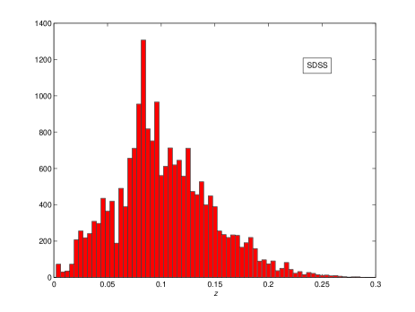
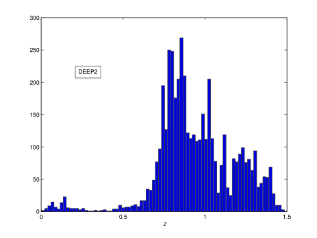
Figure 1: The redshift distribution for both of the samples considered in this work. The median redshifts of SDSS and DEEP2 are $z\sim 0.1$ and $1.0$ respectively.

Current galaxy formation models can be very successful in predicting the general spectral energy distribution (SED) of galaxies at moderate redshifts by evolving stellar population models and co-adding a certain number of stellar populations with different ages (e.g. 2004A&A...425..881L). These models have become mainstream in obtaining stellar population properties (like ages) given current data. With them, constraints can be imposed on the formation times of old elliptical galaxies, the epoch of reionization and cosmology (e.g. 2002ApJ...573...37J; 2004MNRAS.350.1322F).

However most stellar population models do not include the modelling of emission lines in galaxies. This is mainly due to the need for modelling the different phases present in the interstellar medium. Some spectrophotometric codes such as Pegase (2004A&A...425..881L) do include simple prescriptions for emission lines. Other models such as Starburst99 (1999ApJS..123....3L) actually provide equivalent width and flux estimates for the most important emission lines usually observed in galaxy spectra.

The broad band shape of the SED distribution can be related empirically to the presence of an emission line. Roughly speaking, we know that the emission line strength depends on the condition of the gas inside a galaxy; this is strongly related to the amount of star formation ongoing in this galaxy; the star formation can be inferred to a certain extent from the colour, i.e. we know that the SED of a star burst galaxy is much flatter than the corresponding SED of a more passively evolving red galaxy. Therefore the shape of the SED must be correlated in some way to the presence of a strong emission feature in the same galaxy.

We propose to find empirical correlations between the equivalent widths of different lines and the broad band colours from imaging data by utilising novel statistical methods. One method, Artificial Neural Networks, is based on the ANNz code (e.g. 2004PASP..116..345C; 2007ApJ...666..747B; 2007arXiv0705.1437A), previously used to predict photometric redshifts from galaxy colours. The second statistical method we explore here is Locally Weighted Regression (LWR). We can then use such correlations to understand better the process of galaxy formation and the conditions under which strong lines are produced. We suggest that with these statistical results, any model attempting to predict emission features in galaxy spectra could be considerably improved by being calibrated to have the same statistical properties as found in nature.

Another strong motivation for this work is the predictability of an emission feature present in high redshift galaxies. The Sloan Digital Sky Survey (SDSS) and the 2dF Galaxy Redshift Survey (2dFGRS) have probed the nearby Universe. More current (VVDS and DEEP2) as well as future efforts will attempt to probe a large part of the high redshift Universe. More specifically if one is only interested in redshift surveys and not on the more specific SED of a galaxy then it is important to minimize the amount of time spent looking for a galaxy redshift. The most efficient way of doing this is to perform redshift surveys targeted at emission line objects. If there is a possibility of predicting statistically which galaxies have strongest emission lines then the potential time spent locating all these galaxies in redshift space can be reduced and the scope for larger surveys increased in the same way. These approaches would be useful in particular for the forthcoming FMOS survey (2006SPIE.6269E.136D) and the planned WFMOS survey.

The outline of this paper is as follows. In Sec.2 we present the data used to provide correlations found, we examine a low redshift sample (SDSS) as well as a high redshift sample (DEEP2). Section 3 presents the methodology used to extract the correlations from the data and describes the results found, we attempt to use LWR and ANNz for this purpose. In Section 4 we present methodology for classification of AGNs and starforming galaxies. We comment on the prospects that this technique has in speeding up future redshift surveys in Section 5 and conclude in Section 6. We also provide two short appendices describing the mathematics of the LWR and ANNz methods used.

2 The data

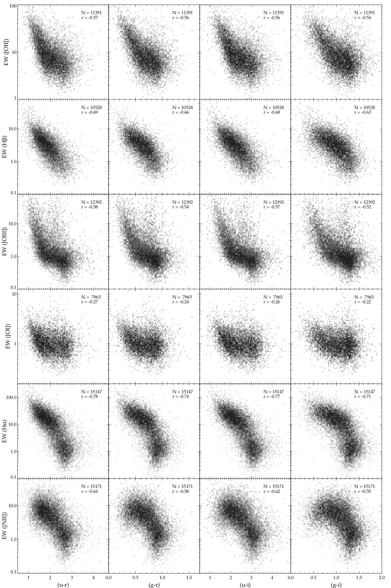
Figure 2: Equivalent widths of the emission lines [O ii], H$\beta$, [O iii], [O i], H$\alpha$, and [N ii], measured from the SDSS spectra as a function of the colours (u-r), (g-r), (u-i), and (g-i). The top-right numbers are the total number of galaxies in each panel and the Spearman rank correlation coefficient. The grey scale level represents the number of galaxies in each pixel, darker pixels having more galaxies.

2.1 SDSS

The low redshift data used in this work is a small sample taken from the SDSS Data Release 2 (2004AJ....128..502A). Photometry is available for all galaxies in five optical bands ($u$, $g$, $r$, $i$ and $z$). We considered the same flux limited sample described in (2006MNRAS.tmp..840S). This is a random sample of 20000 galaxies with reddening-corrected Petrosian r-band magnitudes $r\leq 17.77$, and Petrosian r-band half-light surface brightness $\mu_{50}\leq 24.5$ mag arcsec^-2 (2002AJ....124.1810S). As a quality cut, we selected only the objects that show a signal-to-noise (S/N) ratio greater than 5 in the $g$, $r$ and $i$ bands. We plot the redshift distribution of this sample in Fig.1.

The SDSS spectra used here cover the wavelength range $3800$–$9200$ Å, and have a spectral resolution of $\sim 1800$. They were taken with the standard 3 arcsec diameter fibres in the SDSS spectrograph. The spectra are first corrected for Galactic extinction using the maps of 1998ApJ...500..525S and using the extinction law of 1989ApJ...345..245C. They are then brought to the rest frame and resampled from 3400 to 8900 Å in steps of 1 Å with a flux normalization by the median flux in the $4010$–$4060$ Å region. These procedures are necessary to the spectral analysis described in section 2.3

2.2 DEEP2

The data sample used at high redshift was the DEEP2 first data release (2003SPIE.4834..161D). The DEEP project is an ongoing project, producing spectroscopy for targets at a redshift range $0.75<z<1.5$. The surveys uses the DEIMOS spectrograph (2003SPIE.4841.1657F) on the Keck II telescope and aims to target around 40000 galaxies over 3 square degrees. The targets are pre-selected from imaging with B, R and I filters taken with the CFH12k camera on the Canada-France-Hawaii telescope (e.g. 2004ApJ...609..525C). Galaxies are imaged in $B$, $R$ and $I$ bands and selected to $R_{AB}<24.1$. Furthermore, a colour-cut is applied to pre-select high-redshift objects above a redshift of $z>0.7$ and only $\simeq$ 3 per cent of galaxies above this redshift are rejected by the colour cut. The spectra are taken at moderately high resolution ($R\sim 5000$) and span the range $6300<\lambda<9100$ Å. Hence the doublet [O ii]$\lambda$3727 is found from $0.7<z<1.4$. This sample contains 4681 objects and its redshift distribution is plotted in Fig.1.

2.3 Emission line measurements

In order to measure the emission lines from the SDSS and DEEP2 galaxy spectra we have used a code to fit them as Gaussian functions, composed of three parameters: width, offset (with respect to the rest-frame central wavelength) and flux. In the case of the SDSS sample, we measured emission lines using the methods of described in detail by 2005MNRAS.358..363C and 2006MNRAS.370..721M. The following emission lines have been measured: [O ii], H$\beta$, [O iii], [O i], H$\alpha$, and [N ii]. Lines from the same ion are assumed to have the same width and offset, and we consider the following flux ratio constraints: [O iii]$\lambda 5007$/[O iii]$\lambda 4959=2.97$ and [N ii]$\lambda 6584$/[N ii]$\lambda 6548=3$. To measure the intensities of emission lines we have to remove the stellar contribution in the continuum at their wavelength range, mainly to account for absorption features in the emission line regions. This is done by computing for each SDSS galaxy a synthetic stellar spectrum obtained from a linear combination of simple stellar population spectra that fits the observed continuum in the whole spectral range (after removal of the zones of emission lines and bad pixels). Removing this synthetic spectrum from the observed one leaves us with a pure emission line residual spectrum from which we can easily measure the emission lines. This method provides a reliable estimate of the stellar absorption in the entire spectrum, including the windows where emission lines are found. This procedure is very important since the regions of some emission lines (mainly the H$\alpha$ and H$\beta$ Balmer lines) can be contaminated by strong absorption features which may reduce the equivalent width of the lines. For lines which have no absorption this should make no difference. We also have compared results with integrating over the spectrum and comparing it to the continuum and results do not change much showing that the method is robust.

For the DEEP2 data, only the [O ii] line provided suitable measurements. Moreover, we have adopted a distinct approach to measure this emission line. Instead of fitting the continuum with a synthetic spectrum we have performed a polynomial fit of two continuum windows ($3653$–$3713$ and $3741$–$3801$ Å) around the line. The emission line was then measured from the continuum subtracted spectrum through the Gaussian fitting procedure.

3 Methodology: Predicting emission features with broad band photometry

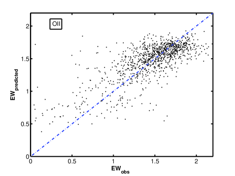
Figure 3: The scatter plot for the 1100 galaxies that were used as a testing set for the prediction of the equivalent width of the [O ii] line in the DEEP sample. The Artificial neural network method used in this plot. We can see a correlation in the log of the predicted equivalent width and the actual measurement. The scatter in the log is of 0.27. Similar results with virtually the same scatter are found with the LWR technique.

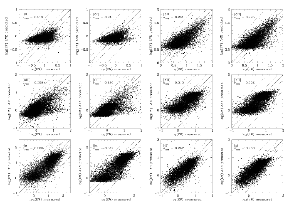
Figure 4: The scatter plot of the log of the real equivalent width versus the predicted equivalent width of galaxies for different lines. For all the plots we have used only galaxies in the testing set which have not made part on the training of the machine learning algorithm that has made the prediction. We present here results using both methods described in this paper. As we can see the results found with both results are comparable and we found no evidence that one method performed better than the other given the data volume available. We can also see that some lines present a better correlation than others and that generally recombination lines are better predicted than collisional lines.

It is well know that galaxy colours present a good correlation with the emission line properties of galaxies, such as their equivalent widths (EW). We illustrate this in Fig. 2, where the equivalent widths of emission lines measured from the SDSS spectra are plotted as a function of various galaxy colours. Several correlations can be identified between these quantities, as confirmed by the high values of the Spearman rank correlation coefficients obtained for some of them, particularly those involving the H$\alpha$ and H$\beta$emission lines. Therefore, it is not only the 4000 Å break colour indice that encodes information about the emission features in galaxies (e.g. Mateus et al. 2006), as typical galaxy colours can also be used to infer these properties in a convenient manner, from photometric data only. On this basis, here we use different methods to combine all information available in the galaxy colours to produce an empirical relation between colours and emission strength.

We have analyzed the data with two different techniques to reinforce the robustness of the correlations found and to compare the two techniques used. We have used Artificial Neural Networks (Bishop), as implemented in the publically available ANNz code (Collister & Lahav 2004 and refereneces therein) and a Locally Weighted Regression (LWR) (LWR). See the Appendices for the mathematical details and implementation of these methods.

Both of the techniques we present here rely on a training set which is representative of the true population of galaxies in order to retrieve the information on the line features in each galaxy. We have separated the sample into two groups, one group which we have used to train the machine learning algorithms and a second sample which we will name the testing set which is set aside and then used to test the reliability of the methods. We have set aside 1100 galaxies in DEEP and 14000 galaxies in the SDSS as testing sets.

The rest of the sample was used as to train the algorithms, that is 2000 galaxies to train in the DEEP sample and 6000 galaxies to train in the SDSS sample. For both methods used here we have to subdivide this sample into a training sample and a validation sample. In the case of neural networks this is done to prevent over-fitting. In the case of the LWR method, this is done to obtain the best kernel value K which is appropriate to the data. Both prescriptions are explained in the Appendix. The architecture of the neural network used is described in the Appendix and is of the type N:2N:2N:1 where N is the number of magnitudes available which is three in the case of DEEP data and five in the case of SDSS.

With the DEEP sample the only line which we have produced a fit for was the [O ii] line. We have performed this analysis only on this line because the DEEP survey relies heavily on the [O ii] line for redshift estimation, therefore having a high completeness. Other lines do not appear in a large fraction of the galaxies in the entire sample. In the sample from SDSS we performed this analysis for all measured lines: [O ii], H$\beta$, [O iii], [O i], H$\alpha$, and [N ii].

We plot in Fig.3 our attempts to recover the equivalent width of the [O ii] line in the DEEP survey using broad band photometry only. We have plotted a scatter plot of the real equivalent width versus the predicted equivalent width for the testing set given the training set. As we can see the logarithm of the equivalent width is predicted reasonably well and show that this weak correlation can be inferred very well with the techniques we have proposed here. We can predict the log of the equivalent width with an error of 0.27 without any spectroscopic information on the redshift of each galaxy.

We present in Fig.4 the results we find by fitting different line widths to SDSS galaxies. Again in these plots we have used only galaxies in the testing set which have not been used in the training process. We find that some line equivalent widths are relatively well predicted by galaxy magnitudes and colours. This is the case for the hydrogen lines where a reasonably strong correlation was found. We have found however that the collisional lines observed are harder to predict. For instance the [O i] line equivalent width had virtually no correlation with any combination of the colours and magnitudes found.

We compare results for both of the techniques using the same testing sets in Fig.4. We plot them side by side so that we can see the relative comparison between the neural network non-linear fit to the data and the locally linear regression used. We have inspected the data and found that there was no significant difference between both methods. Both predictions have yielded results with a very similar scatter given the data volume available. We conclude that for fitting purposes neural networks and a Locally Weighted Regression performs well and on an equal footing.

We have also attempted to simply classify objects into line-emitting and non line-emitting. We have made this separation for each galaxy upon the simple criterium: whether an emission line is detected above a certain value. This separation has been done for each line emission analyzed. For instance if a certain galaxy has an [O i] line but does not posses an H$\alpha$ line then it is considered as an emitting object for the purpose of the analysis on the [O i] line but it is considered as a non-emitting object for the purposes of the H$\alpha$ line analysis.

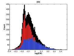
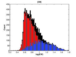
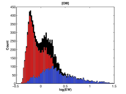
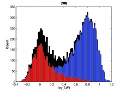
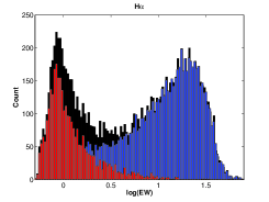
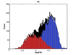
Figure 5: Histograms of the log of the equivalent width for SDSS galaxies. Each plot represents the results for one line. The black histogram are for all the objects for which a line was detected in the analysis of the SDSS data. we have then chosen a median value for the log of the equivalent width for these lines and separated the black samples into a sample with predicted equivalent width higher than this median value and a sample with the predicted value lower than this median value. This shows the amount of overlap that there is in predicting line features with the methods proposed. We can clearly see bi-modality of galaxies and by looking at the H$\beta$ results we can also see that our methods go further than simply detecting this bi-modality clearly separating objects with high and low equivalent width.

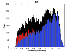
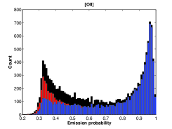
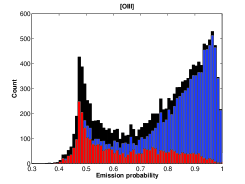
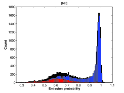
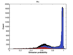
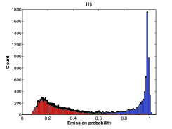
Figure 6: Histogram of the probability that a galaxy is a line-emitting galaxy or a non line-emitting galaxy given by the neural networks. The black histogram represent the entire population. The red and blue histograms represent the line emitting objects and the non line emitting objects. We can see that we can clearly separate the blue and red points for some of the cases whereas other lines cannot be diagnosed with this method.

We have then used the training set in the following way: we have assigned the value of one to emitting objects and the value of zero to ’non-emitting’ objects, defined by the line being detected in our code above a signal to noise of three. A neural network was then trained in this specific training set. When a neural network is trained by binary values between zero and one, it returns a probability (e.g. Lahav et al. 1996 and refereces therin) of that given object belonging to the class described by the binary number. So in our case the value returned by the neural network will be the probability of that object having the emission feature tested for. We have also attempted to perform the same analysis with the LWR technique but found that despite the LWR technique producing predictive results which are comparable and as good as the neural network fit it was not able to perform this classification task nearly as well as the neural networks. This was to be expected as the LWR method is not directly applicable to classification tasks. This is because the linear fit results are not representative of a probability range in the same way the neural networks are.

We plot these results in Fig.6. We can see that the results are varied and depend on the emission line being assessed. For instance there is a good prospect of training a neural network to distinguish between Hydrogen emitters and [N ii] emitters at low redshift but on the other hand the [O i] line exhibits a very poor correlation between colours and magnitudes and its EW. The other oxygen lines exhibit some correlation that are picked up by our methods.

In order to have an idea of what contamination would be introduced but performing a selection based on the predicted equivalent width of a galaxy with our method, we have plotted histograms for the entire sample and then chosen the center of the distribution of the equivalent widths in log space. We have then plotted the histograms for the samples with high predicted equivalent width and low predicted equivalent width in Fig.5.

While predicting the equivalent widths for these emission lines we have found the already known result of galaxy bi-modality. We know that galaxies are bimodal and that late type galaxies have higher star formation rates and therefore stronger emission features whereas the opposite is true for late type galaxies. We can see this bi-modality in the histogram of the equivalent widths for the different lines in Fig.5. This is not found on every set of lines because there are selection effects (fainter lines are simply not seen in some galaxies). For instance the ratio of the H$\alpha$ and H$\beta$ lines for a single galaxy should be roughly constant just below three. This is because both lines are recombination lines and the temperature dependence of the emissivity is roughly the same for both lines. However we do not find this bimodality for H$\beta$ but we find it for H$\alpha$. This is simply because the H$\beta$ flux is smaller and this makes so that a lot of the fainter lines remain undetected. Furthermore we argue that the correlations found in H$\beta$ are strong which suggests that the method we are using is going beyond simply separating the bi-modality and is classifying the line widths according to their size.

4 Methodology: AGN/Star-Formation Classification

4.1 Traditional Spectral galaxy classification

We adopted a traditional procedure to classify galaxies according to their emission line properties. By examining diagnostic diagrams formed by line ratios of optical emission lines, such as the [O iii]/H$\beta$ versus [N ii]/H$\alpha$ diagram proposed by 1981PASP...93....5B, we can distinguish emission-line galaxies according to the mechanism responsible for producing the lines. In such diagrams, hosts of active nuclei (AGN) and star-forming galaxies form two very distinct branches, or wings, making easier the task to separate them. We use this ‘convenient’ diagram to classify galaxies following the classification scheme discussed in 2006MNRAS.tmp..840S based on a theoretical curve used to distinguish galaxies with pure star-formation from those objects with some contribution from nuclear activity to the line intensities. Galaxies below such a curve are classified as normal star-forming galaxies (SF). In addition, we have also used the empirical curve proposed by 2003MNRAS.346.1055K to identify the AGN hosts. Galaxies between the two curves are hybrid objects (the contribution of the AGN to the H$\beta$emission of galaxies below the Kauffmann et al. line is at most 3 per cent) and therefore will not be included in our analysis. The AGN hosts are then selected as those objects located above the Kauffmann et al. empirical curve.

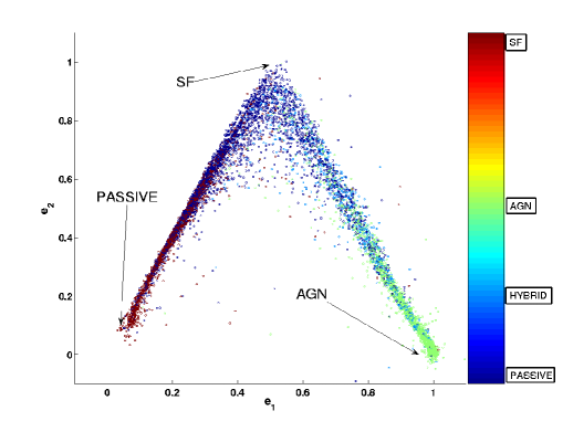
Figure 7: Classification of objects as AGN, SF or passive objects via neural networks. the points are colour coded according to the spectral classification blue, green, orange, red noting passive galaxies, AGN, hybrid objects and star forming galaxies respectively. Each classification has been assigned a doublet in the following way: passive galaxies (0,0), AGN (1,0), SF galaxies (0,1) and hybrid objects (0.5,0.5). The neural networks has been used to estimate this and each point is a galaxy is plotted at $(e1,e2)=(e1+e2/2)\,{\bf i}+e2\,{\bf j}$. As we can see it is possible to predict AGN features from broad band photometry well. There is a degeneracy between the colours of many passive galaxies and star forming ones but it is in general possible to classify them with colours only. As expected hybrid objects lie on the line between AGN and SF galaxies.

4.2 Automated Spectral galaxy classification

In this subsection we attempt to classify the spectral features instead of simply predicting the equivalent width of lines. We have described in Sec.4.1 how we separate galaxies with emission features into AGN or star forming (SF) galaxies.

We have separated the 20000 SDSS galaxies we used in this paper into the following classes: passive galaxies, AGN, star forming galaxies and hybrid objects. Some objects were not classified by the code analysing the spectroscopic data and we have removed those galaxies. We have associated a doublet $(e1,e2)$ to each one of these categories in the following way: passive galaxies (0,0), AGN (1,0), SF galaxies (0,1) and hybrid objects (0.5,0.5).

We have then used a neural network with 5 input nodes, 2 hidden layers with 10 nodes in each layer and 2 output nodes to classify galaxies into AGN, passive galaxies and SF galaxies according to the doublets assigned above. We have used only photometry to perform the training. We used 5000 galaxies for training and 3000 for validating the network. The remaining galaxies were plotted as a testing set in Fig.7. The network returned a doublet for each galaxy. For visual reasons, we plot the doublets in the following basis $(e1,e2)=(e1+e2/2)\,{\bf i}+e2\,{\bf j}$, so that the labels AGN, SF galaxies and passive galaxies are on the corners of an equilateral triangle.

As we can see from Fig.7, there is a trend on the distribution of points in this $(e1,e2)$ diagram. The distribution does not infer a transition between Passive galaxies to SF galaxies to AGN. It indicates that the colour data is able to make a good distinction between passive galaxies and AGN, there is a relativelly good distinction between AGN and SF galaxies and a certain overlap between passive and SF galaxies, which we had already found attempting to classify galaxies in the previous section. This offers an alternative to classifying objects photometrically as AGN or star forming galaxies via a training set and broadband photometry only.

5 Prospects for future surveys.

We have shown that it is possible to predict emission features using broad band photometry. We find that the correlations vary in strength from line to line. Particularly recombination lines are more predictable than collisional lines. We have not included any information on the shape or size of the galaxies. We expect that the results found here would be stronger if information such as shapelet coefficients for galaxies is included into the analysis as we know that galaxies with different star formation rates and therefore different line strengths have different morphologies.

We argue that this technique can be used in future spectroscopic redshift surveys to speed them up. Future facilities such as FMOS or WFMOS will produce spectroscopic surveys in the optical and the IR part of the spectrum targeting mainly the [O ii] and the H$\alpha$ lines. We have shown here that there is a reasonable predictability of the [O ii] line at high redshift and that the H$\alpha$ and H$\beta$ line are well predicted in the low redshift Universe. A high redshift complete sample of around 10000 objects could be used to train a network to then select the preferred targets.

If one chooses to predict the line strengths one alternative would be to fit stellar population synthesis models to the observed spectrum and from that infer a star formation rate and therefore a line flux. We argue that the technique we have proposed here is complementary and one would be able to encode information on the morphology of the galaxy easily whereas if one fits stellar population models to the training data it would be hard to include special information in the analysis.

6 Concluding remarks

We have looked, in this paper, for empirical relations between the equivalent width for several different lines and the broad band colours for the same objects. We used an automated way to explore the correlations found in the data via the use of LWR and ANN. The two methods give very similar results.

We have performed the analysis in two samples, a low redshift sample obtained from the Sloan Digital Sky Survey covering the nearby Universe and a high redshift sample from the first data release of the DEEP survey covering a deeper sample off the Universe. We found that in the DEEP data one could predict the equivalent width of the [O ii] line relatively well by looking at broad band colours only. With the SDSS data six lines were predicted from a training set sample. In general collisional lines presented little correlation although some of them were reasonably predicted by the colours. There was a stronger correlation found in recombination lines.

We have compared the power of prediction of both methods used. We have concluded that both Artificial Neural Networks and the Locally Weighted Regression methods are capable of recovering most of the information encoded in the training set with little statistical difference between both methods. We have used both methods for classification purposes and found that the Neural Networks are capable of classifying the objects into line-emitting and non line-emitting but that the Locally Weighted Regression method was unable to do so. We have shown that it is possible to classify galaxies into AGN, passive galaxies and line emitting galaxies well without galaxy spectra, using solely colours and a training set of the order of 15000 galaxies.

We have discussed the prospects of speeding up redshift surveys with this and we conclude that with a reasonable training set of the order of 10000 galaxies one would be able to considerably speed up future surveys done with instruments such as FMOS and WFMOS. Furthermore, in this paper we have only taken advantage of the colour data; however the methods described can accommodate very easily other information such as morphology or size.

Appendix A Locally weighted regression

Locally Weighted Regression (LWR) is a machine learning method capable of mapping complex, non-linear relations between variables (LWR).

Like any other global fits, LWR minimises a quantity related to the chi-square. The difference is that each data point of the training set has a corresponding weight, which depends on a given query point. Thus, the fitting parameters are valid only locally for that particular query point. In this method any data available for the machine learning would be separated into a training set and a validation set.

In this method, the quantity to be minimised for each query point is given by

$$E=\sum_{i}w_{i}^{2}(y_{i}-f(\mathbf{x_{i}}))^{2}$$ (1)

where $f$ is the linear function to be fitted for the weights for each point $w_{i}$ depend on the distance between the query point and the data point of the training set. The sum over i is performed for each point of the training set. Here the weights have been chosen to follow

$$w_{i}={\rm exp}\,(-{\rm D}^{2}(\mathbf{x_{i}},\mathbf{x_{q}})/2K^{2})$$ (2)

where the function D is the Euclidean distance between the query point $x_{q}$ and the training data point $x_{i}$. The parameters $K$ is called the kernel width, related to the width of the Gaussian determining the weights. For reasonable values of $K$ only the data near the query point have significant contribution to the local fit. The optimal value for the parameter $K$ for a given training set is found by minimising the error found in a validation set. In the training stage many kernel values are attempted and the one which produces best results for the validation set is chosen and fixed. Once K is chosen with the aid of the training and validation set, one is left to define how $f$ is chosen.

We choose to expand the fitting function f

$$f(x)=\beta_{1}t_{1}(x)+\beta_{2}t_{2}(x)+...+\beta_{M}t_{M}(x)$$ (3)

where the functions $t_{i}$ are formed by linear combinations of the inputs $x_{i}$; i.e. $t_{1}=1$, $t_{2}=x_{1}$, $t_{3}=x_{1}^{2}$, and so forth. This equation can be written as

$$f(x)=\mathbf{\beta}^{T}\mathbf{t}(x)$$ (4)

where $t(x)$ is the vector of polynomial terms. Here the weights are recomputed according the distance between points $x_{k}$ and the query point and the matrix $\beta$ is computed according to

$$\mathbf{\beta}=(\mathbf{X}^{T}\mathbf{X})^{-1}\,\mathbf{X}^{T}y$$ (5)

where

$$(\mathbf{X}^{T}\mathbf{X})_{ij}=\sum_{k=1}^{N}w_{i}^{2}t_{i}(x_{k})t_{j}(x_{k})$$ (6)

and

$$(\mathbf{X}^{T}y)_{i}=\sum_{k=1}^{N}w_{i}^{2}t_{i}(x_{k})y_{i}$$ (7)

hence we can solve for the best solution by using a Cholesky decomposition (1992nrfa.book.....P). Now that the $\mathbf{\beta}$ vector and the kernel are chosen we simply apply the relation using the testing set as the query points.

Appendix B Artificial neural networks

We use a particular species of ANN known formally as a multi-layer perceptron (MLP). A MLP consists of a number of layers of nodes (Fig. 8; see e.g. Bishop, and references therein, for background). The first layer contains the inputs, which in this paper are the magnitudes, $m_{i}$, of a galaxy in a number of filters (for ease of notation we arrange these in a vector $\mathbf{m}\equiv(m_{1},m_{2},...,m_{n})$). The final layer contains the outputs; here the equivalent width or emission probability. Intervening layers are described as hidden and there is complete freedom over the number and size of hidden layers used. The nodes in a given layer are connected to all the nodes in adjacent layers. A particular network architecture may be denoted by $N_{\mathrm{in}}$:$N_{1}$:$N_{2}$: $\ldots$ :$N_{\mathrm{out}}$ where $N_{\mathrm{in}}$ is the number of input nodes, $N_{1}$ is the number of nodes in the first hidden layer, and so on. For example 9:6:1 takes 9 inputs, has 6 nodes in a single hidden layer and gives a single output.

Each connection carries a weight, $w_{ij}$; these comprise the vector of coefficients, $\mathbf{w}$, which are to be optimised. An activation function, $g_{j}(u_{j})$, is defined at each node, taking as its argument

$$u_{j}=\sum_{i}w_{ij}g_{i}(u_{i}),$$ (8)

where the sum is over all nodes $i$ sending connections to node $j$. The activation functions are typically taken (in analogy to biological neurons) to be sigmoid functions such as $g_{j}(u_{j})=1/[1+\exp{(-u_{j})}]$, and we follow this approach here. An extra input node – the bias node – is automatically included to allow for additive constants in these functions.

For a particular input vector, the output vector of the network is determined by progressing sequentially through the network layers, from inputs to outputs, calculating the activation of each node (hence this type of neural network is often referred to as a feed-forward network).

Given a suitable training set of galaxies for which we have both photometry, $\mathbf{m}$, and here the Equivalent width, $EW_{\mathrm{train}}$, the ANN is trained by minimising the cost function

$$E=\sum_{k}(EW_{\mathrm{out}}(\mathbf{w},\mathbf{m}_{k})-EW_{\mathrm{train},k})^{2},$$ (9)

with respect to the weights, $\mathbf{w}$, where $EW_{\mathrm{out}}(\mathbf{w},\mathbf{m}_{k})$ is the network output for the given input and weight vectors, and the sum is over the galaxies in the training set. To ensure that the weights are regularised (i.e. that they do not become too large), an extra quadratic cost term

$$E_{\mathrm{w}}=\beta\sum_{i,j}w_{ij}^{2},$$ (10)

is added to equation 9.

Figure 8: A schematic diagram of a multi-layer perceptron, as implemented by annz, with input nodes taking, for example, magnitudes $m_{i}=-2.5\log_{10}f_{i}$ in various filters, a single hidden layer, and a single output node. The architecture is $n$:$p$:1 in the notation used. Each connecting line carries a weight $w_{ij}$. The bias node allows for an additive constant in the network function defined at each node. More complex networks can have additional hidden layers and/or outputs. Here the equivalent width takes the same role as the redshift.

We use an iterative quasi-Newton method to perform this minimisation. Details of the minimisation algorithm and regularisation may be found in Bishop and 1996MNRAS.283..207L.

After each training iteration, the cost function is also evaluated on a separate validation set. After a chosen number of training iterations, training terminates and the final weights chosen for the ANN are those from the iteration at which the cost function is minimal on the validation set. This is useful to avoid over-fitting to the training set if the training set is small. The trained network may then be presented with previously unseen input vectors, and the outputs computed.

To implement the ANNs code to our problem all that is needed is to regard the output node as the equivalent width instead of as the redshift. In this work we found it optimal to work with the log(EW).