Strings in strongly correlated electron systems

Abstract

It is shown that strongly correlated electrons on frustrated lattices like pyrochlore, checkerboard or kagomè lattice can lead to the appearance of closed and open strings. They are resulting from nonlocal subsidiary conditions which propagating strongly correlated electrons require. The dynamics of the strings is discussed and a number of their properties are pointed out. Some of them are reminiscent of particle physics.

Strongly correlated electrons are a subject of intense investigation by many theory groups. Part of that big interest is due to the fact that the corresponding materials have often physical properties which make them attractive for applications. The high-T_c superconducting cuprates Kuzmany ; Bednorz ; Plakida95 are perhaps the most prominent examples. But also materials with a giant or collosal magnetoresistance like the manganites have strongly correlated conduction electrons Dagotto ; Imada98 ; Kudasov03 . Other common examples include 4$f$ and 5$f$ electron systems with heavy quasiparticles at low temperatures Stewart ; Norman , although here the practical use of those materials is less obvious.

Distinct from possible practical uses strongly correlated electron systems are challenging many-body systems which are of basic interest, because techniques for dealing with them must be developed which may apply also to other strong coupling theories. We speak of strongly correlated electrons when the mutual Coulomb repulsion of the particles influences their time evolution more strongly than the kinetic energy gain due to delocalization. Hence the strong coupling character of the many-body problem is obvious. The strong coupling limit of an electron system depends on the type of lattice on which the particles are moving as well as on the filling factor, i.e., on the ratio $n$ of electron number $L$ to number of lattice sites $N$. In the limit in which particle hopping between sites is neglected, the ground state is usually degenerate. Of special interest are geometrically frustrated lattices like the pyrochlore lattice, its two-dimensional version the checkerboard lattice or the kagomè lattice. Here the ground state is macroscopically degenerate for most filling factors $n$. Adding the dynamics to such a system reduces the degeneracy to a small number as examples discussed below will show.

The motion of strongly correlated particles underlies a large number of nonlocal subsidiary conditions. They ensure that the repulsive particle interactions which dominate the dynamics remain as small as possible. It will be shown that particle propagation (worldlines) in the presence of those strong nonlocal subsidiary conditions is equivalent to propagation of closed (loops) or open strings, i.e., worldsheets with trivial subsidiary conditions. For example, fully spin-polarized electrons (or spinless fermions) with strong nearest-neighbor repulsion on a pyrochlore or checkerboard lattice at half filling lead to a complete loop covering of the lattice when the ground state is studied. The loops are obtained by connecting the occupied sites of the lattice. Time evolution of loops, i.e., worldsheets is a phenomenon akin to string theory. For a textbook on the theory see, e.g., Ref. ZwiebachBook .

In the following we want to discuss the properties of closed and open strings of some strongly correlated electron systems. We are dealing here with a particularly simple example of a string theory which is numerically solvable. Some of the features it contains are also met in elementary particle physics. That strongly correlated electrons can be related to string theory albeit of a different form as considered here has been realized before in connection with the fractional quantum Hall effect. String theory realizations of the two-dimensional fractional quantum Hall fluid are found, e.g., in Refs. Boyarsky ; Bergmann . The formation of strings in certain spin models has been described in Ref. levin2005 .

I Strings on a checkerboard lattice

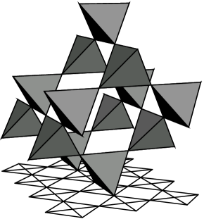
Figure 1: Pyrochlore (above) and checkerboard lattice (below). The latter can be considered as a projection of the former onto a plane (from Ref. Moessner04a ).

(a)

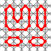
(b)

Figure 2: (a): Loop covering of the checkerboard plane for one of the ground states. The loops are obtained by connecting sites occupied by spinless fermions. The case of half filling is considered. (b): Loop covering in the medial, i.e., square lattice. The same ground-state configuration is shown as in (a).

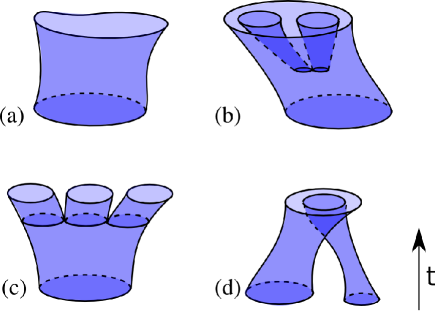
Figure 3: Continuous representation of loop dynamics due to H_eff. (a): time evolution of loops due to B processes which conserve the topology. (b-d): the same for A processes where H_eff induces three kinds of topological changes Pollmann06c .

(a)

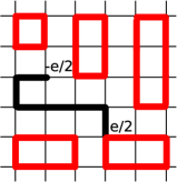
(b)

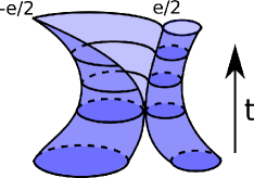
Figure 4: When an energy $\Delta E>V$ is added to the system a loop is broken and an open string is generated. Thereby one end of the string is touching a closed loop. (a): medial lattice with the string shown by a black line. (b): time evolution in a continuous representation.

(a)

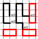
(b)

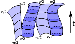
Figure 5: Configuration with two pairs $\left(\frac{e}{2},\frac{e}{2}\right)$ and $\left(-\frac{e}{2},-\frac{e}{2}\right)$ resulting from two particle-antiparticle pairs $\left(\frac{e}{2},-\frac{e}{2}\right)$ with fractional charges $\frac{e}{2}$ (or $-\frac{e}{2}$) of different colors (i.e., sublattice index). (a): on the medial lattice; (b): time evolution of two $\left(\frac{e}{2},-\frac{e}{2}\right)$ pairs and formation of $e$ and $-e$ particles.

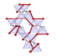
(a) (b)

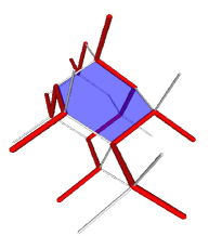
Figure 6: Example of a ground-state configuration of spinless fermions at half filling of a pyrochlore lattice (a) and shown for the medial, i.e., diamond lattice (b). Here particles sit on links of the lattice structure.

The checkerboard lattice can be considered as the two-dimensional version of a pyrochlore lattice. A pyrochlore lattice consists of corner sharing tetrahedra. Each lattice site has six nearest neighbors and the same holds true for the checkerboard lattice (see Fig. 1).

We consider spinless (or fully spin polarized) fermions and half-filling $n=\frac{1}{2}$, i.e., there are twice as many lattice sites $N$ than there are particles. Thus we concentrate exclusively on charge degrees of freedom. The Hamiltonian is

$$H=-t\sum_{\langle ij\rangle}\left(c^{+}_{i}c_{j}+H.c.\right)+V\sum_{\langle ij\rangle}n_{i}n_{j}$$ (1)

with $n_{i}=c^{+}_{i}c_{i}$ and $\langle ij\rangle$ denoting pairs of neighboring sites. We assume strong coupling, i.e., $V\gg\mid t\mid$. In the absence of hopping $(t=0)$ the ground state is macroscopically degenerate with degeneracy $N_{\rm deg}\simeq\left(\frac{4}{3}\right)^{\frac{3}{4}N}$ Lieb67 . Each of the ground states minimizes the repulsive energy $V$ by having two occupied and two empty sites on each of the crisscrossed squares (”tetrahedra”). This is the so-called ”tetrahedron rule” Anderson56 . By connecting nearest-neighbor occupied sites and applying periodic boundary conditions loops are formed. The above subsidiary conditions lead to a macroscopic loop covering of the plane for each of the ground states. For an example see Fig. 2a (each tetrahedron is touched by exactly one loop).

In order to lift the high degeneracy of the ground state by the dynamics of the system represented by $t$, it does not suffice to go to order $t^{2}/V$. In that order dynamical processes contribute equally to all ground states. But the extensive degeneracy is lifted in order $t^{3}/V^{2}$. To that order the effective Hamiltonian becomes Runge04

$$H_{\rm eff}=\frac{12t^{3}}{V^{2}}\sum_{\;\pspicture(0.0pt,2.84526pt)(5.69054pt,8.53581pt)\psset{linewidth=0.85358pt,linestyle=solid}{\psset{}\pspolygon(0.0pt,2.20508pt)(0.0pt,6.40186pt)(3.52814pt,8.53581pt)(7.25545pt,6.40186pt)(7.25545pt,2.20508pt)(3.52814pt,0.0pt)}\endpspicture\;}c^{+}_{j_{6}}c^{+}_{j_{4}}c^{+}_{j_{2}}c_{j_{5}}c_{j_{3}}c_{j_{1}}$$ (2)

where the sum is over all hexagons. The subscripts $j_{1},...,j_{6}$ label the six sites of hexagon $j$. The effective Hamiltonian describes ring hopping on hexagons. It connects different ground states. In order to discuss the remaining degeneracy as well as the properties of strings it helps to go over to the medial lattice which here is the square lattice. It is obtained from the checkerboard lattice by connecting the centers of the crisscrossed squares. In the medial lattice particles sit on links between sites. For illustration a ground-state configuration in the medial lattice is shown in Fig. 2b.

The Hamiltonian (2) for the medial lattice is then written in a pictorial representation Pollmann06c as

$$H_{\rm{eff}} = g\sum_{\{\;\pspicture(5.69054pt,2.84526pt)\psset{linewidth=0.7113pt,linestyle=solid}{\psset{}\psline(2.84526pt,0.0pt)(2.84526pt,2.84526pt)}{\psset{}\pspolygon(0.0pt,0.0pt)(5.69054pt,0.0pt)(5.69054pt,2.84526pt)(0.0pt,2.84526pt)}\endpspicture\;,\;\pspicture(2.84526pt,5.69054pt)\psset{linewidth=0.7113pt,linestyle=solid}{\psset{}\psline(0.0pt,2.84526pt)(2.84526pt,2.84526pt)}{\psset{}\pspolygon(0.0pt,0.0pt)(0.0pt,5.69054pt)(2.84526pt,5.69054pt)(2.84526pt,0.0pt)}\endpspicture\;\}}\Big{(}\big{|}\;\pspicture(17.07164pt,5.69054pt){\psset{linecolor=black,dotsize=2.84526pt 0.0}\psdots(4.2679pt,0.0pt)(4.2679pt,8.53581pt)(17.07164pt,4.2679pt)}\psset{linewidth=0.85358pt,linestyle=dotted}{\psset{}\psline(8.53581pt,0.0pt)(8.53581pt,8.53581pt)}{\psset{}\pspolygon(0.0pt,0.0pt)(17.07164pt,0.0pt)(17.07164pt,8.53581pt)(0.0pt,8.53581pt)}\psset{linewidth=1.42262pt,linestyle=solid}{\psset{linecolor=black}\psline(0.0pt,0.0pt)(8.53581pt,0.0pt)}{\psset{linecolor=black}\psline(0.0pt,8.53581pt)(8.53581pt,8.53581pt)}{\psset{linecolor=black}\psline(17.07164pt,0.0pt)(17.07164pt,8.53581pt)}\endpspicture\;\big{\rangle}\big{\langle}\;\pspicture(17.07164pt,5.69054pt){\psset{linecolor=black,dotsize=2.84526pt 0.0}\psdots(12.80373pt,0.0pt)(12.80373pt,8.53581pt)(0.0pt,4.2679pt)}\psset{linewidth=0.85358pt,linestyle=dotted}{\psset{}\psline(8.53581pt,0.0pt)(8.53581pt,8.53581pt)}{\psset{}\pspolygon(0.0pt,0.0pt)(17.07164pt,0.0pt)(17.07164pt,8.53581pt)(0.0pt,8.53581pt)}\psset{linewidth=1.42262pt,linestyle=solid}{\psset{linecolor=black}\psline(8.53581pt,0.0pt)(17.07164pt,0.0pt)}{\psset{linecolor=black}\psline(8.53581pt,8.53581pt)(17.07164pt,8.53581pt)}{\psset{linecolor=black}\psline(0.0pt,0.0pt)(0.0pt,8.53581pt)}\endpspicture\;\big{|}-\big{|}\;\pspicture(17.07164pt,5.69054pt){\psset{linecolor=black,dotsize=2.84526pt 0.0}\psdots(4.2679pt,0.0pt)(4.2679pt,8.53581pt)(17.07164pt,4.2679pt)(8.53581pt,4.2679pt)}\psset{linewidth=0.85358pt,linestyle=dotted}{\psset{}\psline(8.53581pt,0.0pt)(8.53581pt,8.53581pt)}{\psset{}\pspolygon(0.0pt,0.0pt)(17.07164pt,0.0pt)(17.07164pt,8.53581pt)(0.0pt,8.53581pt)}\psset{linewidth=1.42262pt,linestyle=solid}{\psset{linecolor=black}\psline(0.0pt,0.0pt)(8.53581pt,0.0pt)(8.53581pt,8.53581pt)(0.0pt,8.53581pt)}{\psset{linecolor=black}\psline(17.07164pt,0.0pt)(17.07164pt,8.53581pt)}\endpspicture\;\big{\rangle}\big{\langle}\;\pspicture(17.07164pt,5.69054pt){\psset{linecolor=black,dotsize=2.84526pt 0.0}\psdots(12.80373pt,0.0pt)(12.80373pt,8.53581pt)(0.0pt,4.2679pt)(8.53581pt,4.2679pt)}\psset{linewidth=0.85358pt,linestyle=dotted}{\psset{}\psline(8.53581pt,0.0pt)(8.53581pt,8.53581pt)}{\psset{}\pspolygon(0.0pt,0.0pt)(17.07164pt,0.0pt)(17.07164pt,8.53581pt)(0.0pt,8.53581pt)}\psset{linewidth=1.42262pt,linestyle=solid}{\psset{linecolor=black}\psline(17.07164pt,0.0pt)(8.53581pt,0.0pt)(8.53581pt,8.53581pt)(17.07164pt,8.53581pt)}{\psset{linecolor=black}\psline(0.0pt,0.0pt)(0.0pt,8.53581pt)}\endpspicture\;\big{|}\Big{)}$$ (3)

$$= g\sum_{\{\;\pspicture(5.69054pt,2.84526pt)\psset{linewidth=0.7113pt,linestyle=solid}{\psset{}\psline(2.84526pt,0.0pt)(2.84526pt,2.84526pt)}{\psset{}\pspolygon(0.0pt,0.0pt)(5.69054pt,0.0pt)(5.69054pt,2.84526pt)(0.0pt,2.84526pt)}\endpspicture\;,\;\pspicture(2.84526pt,5.69054pt)\psset{linewidth=0.7113pt,linestyle=solid}{\psset{}\psline(0.0pt,2.84526pt)(2.84526pt,2.84526pt)}{\psset{}\pspolygon(0.0pt,0.0pt)(0.0pt,5.69054pt)(2.84526pt,5.69054pt)(2.84526pt,0.0pt)}\endpspicture\;\}}\Big{(}\big{|}A\big{\rangle}\big{\langle}\overline{A}\big{|}-\big{|}B\big{\rangle}\big{\langle}\overline{B}\big{|}\Big{)}$$

with $g=\frac{12t^{3}}{V^{2}}$. The two ring-hopping processes differ with respect to the site in the center of the flipable plaquette. It is either empty (process A) or occupied (process B). For identification of conserved quantities we divide the links of the square lattice into four sublattices 1, …, 4. It is seen immediately that H_eff conserves the total number of particles (loop segments) on each sublattice $N_{1},...,N_{4}$. Moreover $N_{1}-N_{3}$ and $N_{2}-N_{4}$ are also conserved. Note that the latter two quantities are also conserved when higher order processes in $t/V$ are included while that is not the case for $N_{1},...,N_{4}$ separately. The quantities $(N_{1}-N_{3})$ and $(N_{2}-N_{4})$ are related to the gradients $\chi_{x}$ and $\chi_{y}$ of a height field $h(x,y)$ Bloete82 . A height representation does apply here since the Hilbert space on which H_eff acts is equivalent to that of the six-vertex model BaxterBook .

Returning to (3) we note that the sign of $g$ is unimportant since it can always be changed by a proper gauge transformation of the basis states Pollmann06c . The relative sign in (3) results from a difference in the occupation of the central site of the plaquette, when A and B processes are accounted for. But as pointed out in Ref. Boyarsky also that sign can be changed by a special gauge transformation so that we do not face here the well-known fermionic sign problem. While processes of the form $\mid B\rangle\langle\bar{B}\mid$ in H_eff do not change the topology of a closed string (loop) configuration processes of the form $\mid A\rangle\langle\bar{A}\mid$ do so. As discussed in Ref. Boyarsky one loop can go over into three separate loops or two loops inside a third one and vice versa. Also two separate loops can go over into one loop inside a second one and vice versa. When the time evolution exp$\left[-i\tau H_{\rm eff}\right]$ of the loops is considered one obtains world sheets instead of world lines. Because of the square lattice structure spatial changes are discretize. When the continuum limit is taken the loops or closed strings show a time evolution which has the form of world sheets and is schematically shown in Fig. 3. While Fig. 3a correspondents to B processes, Figs. 3b-d result from A processes. The fluctuating loops depicted in that figure represent the ground state or the vacuum state of the system. It has been calculated before for finite systems by numerical methods and is well known Pollmann06b .

Next we consider the case when an energy $\Delta E$ is added to the vacuum. When $\Delta E>V$ a loop is broken up and an open string is created. One end of the string is touching a closed loop while the other end is open. At those two points the tetrahedron rule is broken. In the original checkerboard lattice they correspond to crisscrossed square with three particles and with one particle only. Thus at the two ends of the string the charges are $\frac{e}{2}$ and $-\frac{e}{2}$. We may speak also of a particle-antiparticle pair production (see Cheng88 ). A broken loop on the medial lattice is shown in Fig. 4a by the black line. The time evolution of a configuration with loop breaking is shown in Fig. 4b when again the continuous limit is taken.

It was demonstrated in Pollmann06b that a particle pair with charge $+\frac{e}{2}$, $-\frac{e}{2}$ is confined by a constant confining force. This is reminiscent of quarks. Thus a tension $T$ must be associated with the string connecting the two fractions. The string tension was determined to be $T=0.2\mid g\mid$. When a fractionally charged pair is pulled apart so that the confining energy exceeds the threshold value $\Delta E=V$, a new particle-antiparticle pair with $\frac{e}{2},-\frac{e}{2}$ is generated out of the vacuum. This way the energy is lowered. Note the analogy to the generation of $\mu$ mesons, i.e., quark-antiquark production in QCD Cheng88 . Pumping an energy $\Delta E=nV$ into the system generates $n$ pairs with fractional charge $\frac{e}{2},-\frac{e}{2}$. They can combine to form new pairs $\frac{e}{2},\frac{e}{2}$ and $-\frac{e}{2},-\frac{e}{2}$, depending on relative distances of the constituents. Note that a string with charges $+\frac{e}{2},+\frac{e}{2}$ at its ends is touching two closed loops while a string with charges $-\frac{e}{2},-\frac{e}{2}$ at its end is not touching any loops. For a better visualization this is shown in Fig. 5a for two pairs the medial square lattice. The corresponding time evolution of those two pairs $\left(\frac{e}{2},\frac{e}{2}\right)$ and $\left(-\frac{e}{2},-\frac{e}{2}\right)$ is schematically indicated in Fig. 5b.

It should be realized that one must distinguish between two types of pairs $\left(\frac{e}{2},\frac{e}{2}\right)$ and likewise $\left(-\frac{e}{2},-\frac{e}{2}\right)$. One type is equivalent to adding or removing a spinless particle. In that case the fractional charges must sit on different sublattices of the checkerboard lattice. Adding a particle corresponds to converting an empty link into an occupied one which connects two loops (see Fig. 2b). Removing a particle implies taking out a loop segment. In both cases the two lattice sites connected by the link belong to different sublattices. We attach therefore an additional colour index to the fractional particles, e.g., black or white depending on which sublattice of the checkerboard lattice or the medial square lattice they are situated. Pairs corresponding to electrons or holes are colour neutral. They have equal number of black and white fractional parts. This is the case for the pairs shown in Fig. 5. When pairs $\left(\frac{e}{2},\frac{e}{2}\right)$ or $\left(-\frac{e}{2},-\frac{e}{2}\right)$ are not colour neutral they can not reduce to an electron or hole. Instead they have always at least one string between the two constituents. Their energy is higher than the one of an electron or hole.

When due to large values of $\Delta E$ the density of broken loops and hence the generation of fractionally charged particle-antiparticle pairs is sufficiently high, we are ending up with a plasma consisting of particles and antiparticles with fractional charges. Although they are still connected pairwise by strings which act like glue (i.e., gluons), the changes of connections take place so frequently, namely with $|t|$ that the strings must be also considered as part of the plasma.

As $\Delta E$ becomes very large as compared with $V$ the significance of the tetrahedron rule decreases. Not only will there be more and more tetrahedra generated with three particles or one particle but also with four or zero particles. Thus a string description looses its meaning. Instead it is more appropriate to return to a description of the system in terms of electrons with their correlation hole. Since the original loops are completely disrupted the kinetic processes take place on the scale of $|t|$ rather than $|t|^{3}/V^{2}$.

II Other frustrated lattices

(a)

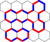
(b)

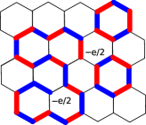
Figure 7: (a): Honeycomb lattice at 1/3 filling with electrons sitting on coloured links, with red/blue referring to spin up/down. (b): Removal of an electron with spin up resulting in an open string with charges -e/2 at each end and a net down spin. This spin is highly nonlocal and distributed over the open string. The latter is a Heisenberg chain with $S_{z}=-1/2$. Figs (a) and (b) differ in addition by a hexagon flipping process.

There exist many geometrically frustrated lattice systems. An instructive overview is found in Diep05 . Two particularly well investigated lattice types are the pyrochlore and the kagomè lattice. As pointed out before the checkerboard lattice and the pyrochlore lattice are closely related, one being the two-dimensional version of the other. We consider spinless fermions on a pyrochlore lattice at half filling described by the Hamiltonian (1). In the absence of hopping, i.e., for $t=0$ the ground state is again macroscopical degenerate. As before we are interested in strongly correlated systems in which case $V\gg|t|$. Like in a checkerboard lattice terms of order $t^{2}/V$ do not lift the degeneracy of the ground state. But terms of order $t^{3}/V^{2}$ do. Therefore an effective Hamiltonian of the form (2) is again applicable for describing the low-energy dynamics of the system. However when ring hopping takes place there is unlike in the checkerboard lattice no site inside the ring. This is seen explicitely by going over to the medial lattice which in this case has the diamond structure. It is obtained by connecting the clusters of neighboring tetrahedra. An example of a configuration with a flipable hexagon in the medial lattice is shown in Fig. 6. Thus processes of type $\mid B\rangle\langle\bar{B}\mid$ found in configurations of the checkerboard lattice are ruled out here. This implies that all fluctuations are accompanied by topological changes in the loop covering. When a particle of charge $e$ is added to the system an unoccupied link changes into an occupied one and the two associated sites have three occupied links ending at them. By hopping processes of order $t$ the two sites with three links separate carrying a charge $\frac{e}{2}$ each. Various authors Balents02 ; Hermele04 predict the existence of a deconfined phase on related dimer/loop models on the diamond lattice. This suggests that deconfined fractional charges on the pyrochlore lattice can exist as conjectured in FuldeP02 . The processes determining the time evolution of the strings are the same as in Figs. 3b-d.

Of interest is also the case of $\frac{1}{4}$ filling. The strong repulsions require that each tetrahedron contains one particle. Its time evolution is governed again by (2). The associated world lines of the particles are subject to strong nonlocal subsidiary conditions, i.e., that every tetrahedron contains exactly one particle. Their propagation is equivalent to that of a string net. This is seen by connecting all empty sites and studying their time evolution as that of a net of strings.

Next we consider a kagomè lattice at $\frac{1}{3}$ filling with electrons obeying an extended Hubbard Hamiltonian

$$H=-t\sum_{\langle ij\rangle\sigma}\left(c^{+}_{i\sigma}c_{j\sigma}+h.c.\right)+V\sum_{\langle ij\rangle}n_{i}n_{j}+U\sum_{i}n_{i\uparrow}n_{i\downarrow}~{}~{}~{}.$$ (4)

We assume $U\rightarrow\infty$ so that double occupancies of sites are excluded and furthermore that $V\gg\mid t\mid$, i.e., that the system is in the strong coupling limit. We eliminate $U$ from the Hamiltonian by replacing $H$ by an extended $t-J$ Hamiltonian Brooks of the form

$$\tilde{H}=-t\sum_{\langle ij\rangle}\left(\hat{c}^{+}_{i\sigma}c_{j\sigma}+h.c.\right)+V\sum_{\langle ij\rangle}n_{i}n_{j}+J\sum_{\langle ij\rangle}\left({\bf S}_{i}{\bf S}_{j}-\hat{n}_{i}\hat{n}_{j}\right)~{}~{}~{}.$$ (5)

Here

$$\hat{c}^{+}_{i\sigma} = c^{+}_{i\sigma}\left(1-n_{i-\sigma}\right)$$

$$\hat{c}_{i\sigma} = c_{i\sigma}\left(1-n_{i-\sigma}\right)$$ (6)

act in the reduced Hilbert space, i.e., one which does not contain doubly occupied sites. Furthermore $\hat{n}_{i}=\sum_{\sigma}\hat{c}^{+}_{i\sigma}\hat{c}_{i\sigma}$ and ${\bf S}_{i}=(1/2)\sum_{\alpha\beta}\hat{c}^{+}_{i\alpha}{\bf\sigma}_{\alpha\beta}\hat{c}_{i\beta}$. The $\bf\sigma$ matrices are the usual Pauli matrices. The spin coupling constant is $J=\frac{4t^{2}}{U}$. The large on-site repulsion U has been replaced by an effective antiferromagnetic spin-spin interaction which accounts for virtual hopping processes by which a site is doubly occupied for a short time. A transformation from (4) to (5) leads to additional terms of order $t^{2}/U$ involving three sites, but they are usually neglected. Clearly $V\gg J$.

The new aspect here is the inclusion of spin degrees of freedom. When $t=0$ the ground state is again macroscopically degenerate. Going over to the medial lattice which is the honeycomb one we connect the occupied links which leads to a loop covering of the plane. The strings forming the loops consist of segments of two different colours in correspondence to the spin of the electrons on the links. This is shown in Fig. 7a for a particular configuration. On each loop the number of up and down spins is equal. The antiferromagnetic interaction favors small loops since the energy per site of a Heisenberg chain with an even number of sites increases with the chain length Bloete86 ; Karbach95 ; Eggert . When the dynamics is included we deal again with ring hopping on hexagons of the form

$$H_{\rm{hex}}=-g\sum_{\left\{\;\pspicture(0.0pt,2.84526pt)(5.69054pt,8.53581pt)\psset{linewidth=0.85358pt,linestyle=solid}{\psset{}\pspolygon(0.0pt,2.20508pt)(0.0pt,6.40186pt)(3.52814pt,8.53581pt)(7.25545pt,6.40186pt)(7.25545pt,2.20508pt)(3.52814pt,0.0pt)}\endpspicture\;\right\}\left\{\blacktriangle\blacksquare\bullet\right\}}\Big{(}\big{|}\;\pspicture(0.0pt,2.84526pt)(9.95845pt,17.07164pt)\psset{unit=21.33957pt}\psset{linewidth=0.64018pt,linestyle=dotted}{\pspolygon(0.0pt,3.20093pt)(0.0pt,9.6028pt)(5.544pt,12.80374pt)(11.08803pt,9.6028pt)(11.08803pt,3.20093pt)(5.544pt,0.0pt)}\psset{linewidth=1.70715pt,linestyle=solid}{\psline(0.0pt,3.20093pt)(0.0pt,9.6028pt)}{\psline(5.544pt,12.80374pt)(11.08803pt,9.6028pt)}{\psline(11.08803pt,3.20093pt)(5.544pt,0.0pt)}{\psset{linecolor=gray,dotsize=4.26791pt 0.0}\psdots(0.0pt,6.40187pt)}{\psset{dotstyle=triangle*,linecolor=gray,dotsize=4.26791pt 0.0}\psdots(8.31602pt,11.20326pt)}{\psset{linecolor=gray,dotsize=4.26791pt 0.0,dotstyle=square*}\psdots(8.31602pt,1.60046pt)}\endpspicture\;\big{\rangle}\big{\langle}\;\pspicture(0.0pt,2.13396pt)(7.46884pt,12.80374pt)\psset{unit=21.33957pt}\psset{linewidth=0.64018pt,linestyle=dotted}{\psset{}\pspolygon(0.0pt,3.20093pt)(0.0pt,9.6028pt)(5.544pt,12.80374pt)(11.08803pt,9.6028pt)(11.08803pt,3.20093pt)(5.544pt,0.0pt)}\psset{linewidth=1.70715pt,linestyle=solid}{\psline(5.544pt,12.80374pt)(0.0pt,9.6028pt)}{\psline(11.08803pt,3.20093pt)(11.08803pt,9.6028pt)}{\psline(5.544pt,0.0pt)(0.0pt,3.20093pt)}{\psset{linecolor=gray,dotsize=4.26791pt 0.0}\psdots(2.772pt,11.20326pt)}{\psset{dotstyle=triangle*,linecolor=gray,dotsize=4.26791pt 0.0}\psdots(11.20326pt,6.40187pt)}{\psset{linecolor=gray,dotsize=4.26791pt 0.0,dotstyle=square*}\psdots(2.772pt,1.60046pt)}\endpspicture\;\big{|}+\big{|}\;\pspicture(0.0pt,2.13396pt)(7.46884pt,12.80374pt)\psset{unit=21.33957pt}\psset{linewidth=0.64018pt,linestyle=dotted}{\pspolygon(0.0pt,3.20093pt)(0.0pt,9.6028pt)(5.544pt,12.80374pt)(11.08803pt,9.6028pt)(11.08803pt,3.20093pt)(5.544pt,0.0pt)}\psset{linewidth=1.70715pt,linestyle=solid}{\psline(0.0pt,3.20093pt)(0.0pt,9.6028pt)}{\psline(5.544pt,12.80374pt)(11.08803pt,9.6028pt)}{\psline(11.08803pt,3.20093pt)(5.544pt,0.0pt)}{\psset{dotstyle=square*,linecolor=gray,dotsize=4.26791pt 0.0}\psdots(0.0pt,6.40187pt)}{\psset{linecolor=gray,dotsize=4.26791pt 0.0}\psdots(8.31602pt,11.20326pt)}{\psset{dotstyle=triangle*,linecolor=gray,dotsize=4.26791pt 0.0}\psdots(8.31602pt,1.60046pt)}\endpspicture\;\big{\rangle}\big{\langle}\;\pspicture(0.0pt,2.13396pt)(7.46884pt,12.80374pt)\psset{unit=21.33957pt}\psset{linewidth=0.64018pt,linestyle=dotted}{\psset{}\pspolygon(0.0pt,3.20093pt)(0.0pt,9.6028pt)(5.544pt,12.80374pt)(11.08803pt,9.6028pt)(11.08803pt,3.20093pt)(5.544pt,0.0pt)}\psset{linewidth=1.70715pt,linestyle=solid}{\psline(5.544pt,12.80374pt)(0.0pt,9.6028pt)}{\psline(11.08803pt,3.20093pt)(11.08803pt,9.6028pt)}{\psline(5.544pt,0.0pt)(0.0pt,3.20093pt)}{\psset{linecolor=gray,dotsize=4.26791pt 0.0}\psdots(2.772pt,11.20326pt)}{\psset{dotstyle=triangle*,linecolor=gray,dotsize=4.26791pt 0.0}\psdots(11.20326pt,6.40187pt)}{\psset{linecolor=gray,dotsize=4.26791pt 0.0,dotstyle=square*}\psdots(2.772pt,1.60046pt)}\endpspicture\;\big{|}+{\rm H.c.}\Big{)}$$ (7)

with $g=6t^{3}/V^{2}$. The sum over the three symbols is taken over all possible color (spin) combinations of a flippable hexagons. The particles can hop either clockwise or counter-clockwise around hexagons. These processes can lead to different configurations, depending on the colors (spins) of the dimers on the hexagon. The evolution of loops with time is the same as the one due to $A$ processes of the checkerboard lattice and therefore of the form shown in Figs. 3b-d. Note that we have here in addition fluctuations of the spins of the loop segments. By writing

$$J\sum_{\langle ij\rangle}\left({\bf S}_{i}{\bf S}_{j}-\frac{\hat{n}_{i}\hat{n}_{j}}{4}\right) = J\sum_{\langle ij\rangle}\left(S^{z}_{i}S^{z}_{j}-\frac{\hat{n}_{i}\hat{n}_{j}}{4}\right)$$ (8)

$$+\frac{J}{2}\sum_{\langle ij\rangle}\left(S^{+}_{i}S^{-}_{j}+S^{-}_{i}S^{+}_{j}\right)$$

we notice that due to the last term on the right-hand side neighboring links can change spins from up-down to down-up (see Fig. 7a).

Next let us remove one electron from the system by eliminating one link in a loop. This results in an open string. At the ends of that string charges $-\frac{e}{2}$ are located. They can separate from each other due to hopping processes. An example is shown in Fig. 7b. The open ended chain contains always an odd number of sites. The ground state of such a Heisenberg chain is two-fold degenerate with total $S_{z}=\pm\frac{1}{2}$. Which of the two possibilities realized depends on the spin of the removed electron. In any case, it is noticed that the spin $\frac{1}{2}$ is now smeared (or distributed) over the open string and is highly nonlocal. The time evolution of the open string follows again the ones in Figs. 3(b-d) but this time with one opened loop at any time $t$.

In passing we note that it was shown in Pollmann07 that the ground state of the system at $\frac{1}{6}$ filling is ferromagnetic with maximum spin $S_{\rm tot}=\frac{1}{2}M$ where $M$ is the total particle number. It was also shown that the ferromagnetic ground state is robust against perturbations. Due to the inclusion of spin degrees of freedom there is now an additional lower energy scale present which is of order $J$. Since we are interested here in pointing out the connections of strongly correlated electrons with strings only, we defer a detailed discussion of this scale to a future investigation.

III Summary

The aim of this paper has been to draw attention to the fact that in strongly correlated electron systems on frustrated lattices the dynamics of the system is given by that of closed and open strings. For simplicity we have assumed in the larger part of the paper that the electrons are fully spin polarized or spinless. That enabled us to focus on charge degrees of freedom. At particular lattice filling factors, the ground state of the system consists of fluctuating loops which cover completely the lattice. The strings are a direct consequence of strong nonlocal subsidiary conditions. In the case of a pyrochlore or checkerboard lattice they take the form of a tetrahedron rule which ensures that nearest-neighbor repulsions of fully polarized electrons remain as small as possible. The time evolution of strings results in world sheets instead of world lines. The dynamics caused by the kinetic energy reduces in the strong-coupling limit considered here to ring hopping processes. This assumes special filling factors like the one mainly considered here of one half.

Dynamical fluctuation lead not only to deformations of loops but a lso to loop formations of different topologies. In the continuum limit, which we consider here, the discrete lattice structure is ignored and enters only in form of the dynamic processes which depend on it. The different topological changes in the loop covering induced by the dynamics have been pointed out and visualized.

When energy is added to such a system which exceeds a threshold value, closed strings, i.e., loops begin to break up. In that case an open string has at its ends two particles with charges $+\frac{e}{2}$ and $-\frac{e}{2}$. This corresponds to half of an electron and half of a hole with respect to the vacuum, i.e., the ground state. The string connecting the two has a string tension which is finite in the two-dimensional checkerboard case but is expected to be zero in the three dimensional pyrochlore lattice. With increasing energy the number of open strings increases and a plasma of fractionalized particles form until the string picture looses its meaning.

When the electron spin is taken into consideration strings are coloured according to the spins of the involved particles. This has been explicitely discussed for a kagomé lattice at $\frac{1}{3}$ filling. Removal of an electron leads to an open string with a spin $\frac{1}{2}$ distributed all over the string. The same holds true when the pyrochlore lattice is considered instead. We are dealing here with a three dimensional system with spin-charge separation. This contradicts common belief that the latter can occur only in low-dimensional systems.

As noticed above strongly correlated electrons on frustrated lattices show features akin to particle physics. It would indeed be strange if nature would realize certain phenomena only in one field of physics and not also in others albeit in varied form.

References

- (1) H. Kuzmany, M. Mehring, and J. Fink, eds., Electronic Properties of High-Tc Superconductors, vol. 113 of Springer Series in Solid State Sciences (Springer, Heidelberg, 1993).
- (2) J. G. Bednorz and K. A. Müller, eds., Superconductivity, vol. 90 of Springer Series in Solid State Sciences (Springer, Heidelberg, 1990).
- (3) N. M. Plakida, High-Temperature Superconductivity (Springer, Heidelberg, 1995).
- (4) E. Dagotto, Nanoscale Phase Separation and Colossal Magnetoresistance: The Physics of Manganites and Related Compounds, vol. 136 of Springer Series in Solid State Sciences (Springer, Berlin, 2003).
- (5) M. Imada, A. Fujimori, and Y. Tokura, Rev. Mod. Phys. 70, 1039 (1998).
- (6) Y. B. Kudasov, Physics-Uspekhi 46, 117 (2003).
- (7) G. R. Stewart, Rev. Mod. Phys. 56, 755 (1984).
- (8) M. R. Norman and D. Koelling, In: Handbook of the Physics and Chemistry of Rare Earth, vol. 17 (Elsevier, Amstersam, 1993).
- (9) B. Zwiebach, A first course in string theory (Cambridge Univ. Press, Cambridge, 2004).
- (10) A. Boyarsky, B. Kulik, and O. Ruchayskiy (2003), eprint arXiv:hep-th/0312242.
- (11) O. Bergmann (2004), eprint arXiv:hep-th/0401106.
- (12) M. A. Levin and X.-G. Wen, Phys. Rev. B 71, 045110 (2005).
- (13) R. Moessner, O. Tchernyshyov, and S. L. Sondhi, J. Stat. Phys. 116, 755 (2002).
- (14) F. Pollmann, J. Betouras, K. Shtengel, and P. Fulde, Phys. Rev. Lett 97, 170407 (2006).
- (15) L. H. Lieb, Phys. Rev. Lett. 18, 692 (1967).
- (16) P. W. Anderson, Phys. Rev. 102, 1008 (1956).
- (17) E. Runge and P. Fulde, Phys. Rev. B 70, 245113 (2004).
- (18) H. W. J. Blöte and H. J. Hilhorst, J. Phys. A 15, L631 (1982).
- (19) R. Baxter, Exactly Solved Models in Statistical Mechanics (Academic, San Diego, 1982).
- (20) F. Pollmann and P. Fulde, Europhys. Lett. 75, 133 (2006).
- (21) T.-P. Cheng and L.-F. Li, Gauge Theory of elementary particle physics (Oxford University Press, USA, 1988).
- (22) H. T. Diep, ed., Frustrated Spin Systems (World Scientific, Singapore, 2005).
- (23) L. Balents, M. P. A. Fisher, and S. M. Girvin, Phys. Rev. B 65, 224412 (2002).
- (24) M. Hermele, M. P. A. Fisher, and L. Balents, Phys. Rev. B 69, 064404 (2004).
- (25) P. Fulde, K. Penc, and N. Shannon, Ann. Phys. (Leipzig) 11, 892 (2002).
- (26) A. B. Harris and R. V. Lange, Phys. Rev. 157, 295 (1967).
- (27) H. W. J. Blöte, J. L. Cardy, and M. P. Nightingale, Phys. Rev. Lett. 56, 742 (1986).
- (28) M. Karbach and G. Müller, J. Phys. A: Math. Gen. 28, 4469 (1995).
- (29) S. Eggert, Priv. comm.
- (30) F. Pollmann, K. Shtengel, and P. Fulde (2007), eprint arXiv:0705.3941.