A Class of Residual Distribution Schemes and Their Relation to Relaxation Systems
Abstract
Residual distributions (RD) schemes are a class of of high-resolution finite volume methods for unstructured grids. A key feature of these schemes is that they make use of genuinely multidimensional (approximate) Riemann solvers as opposed to the piecemeal 1D Riemann solvers usually employed by finite volume methods. In 1D, LeVeque and Pelanti [J. Comp. Phys. 172, 572 (2001)] showed that many of the standard approximate Riemann solver methods (e.g., the Roe solver, HLL, Lax-Friedrichs) can be obtained from applying an exact Riemann solver to relaxation systems of the type introduced by Jin and Xin [Comm. Pure Appl. Math. 48, 235 (1995)]. In this work we extend LeVeque and Pelanti’s results and obtain a multidimensional relaxation system from which multidimensional approximate Riemann solvers can be obtained. In particular, we show that with one choice of parameters the relaxation system yields the standard N-scheme. With another choice, the relaxation system yields a new Riemann solver, which can be viewed as a genuinely multidimensional extension of the local Lax-Friedrichs scheme. This new Riemann solver does not require the use Roe-Struijs-Deconinck averages, nor does it require the inversion of an matrix in each computational grid cell, where is the number of conserved variables. Once this new scheme is established, we apply it on a few standard cases for the 2D compressible Euler equations of gas dynamics. We show that through the use of linear-preserving limiters, the new approach produces numerical solutions that are comparable in accuracy to the N-scheme, despite being computationally less expensive.
keywords:
residual distribution schemes , relaxation systems , approximate Riemann solvers , finite volume methods , hyperbolic conservation laws1 Introduction
In the last few decades intense research into shock-capturing schemes has resulted in several numerical methods for solving partial differential equations (PDEs) that admit discontinuous weak solutions in the form of shock-waves. Examples of such schemes include WENO (weighted essentially non-oscillatory) [16], central [18], MUSCL (monotone upstream-centered schemes for conservation laws) [27], and wave propagation schemes [19]. One difficulty with these methods is that in general they do not trivially extend to problems in complex geometries. In order to handle application problems where complex geometry is of great importance, three broad classes of strategies have been considered: (1) Cartesian cut-cell methods [15], (2) overlapping meshes [9], and (3) unstructured grid methods. We will focus in this work on the last approach, thus eliminating the problem of cut-cells (1st approach) and interpolation between different grid patches (2nd approach), but requiring some efficient grid generation tool.
On unstructured grids, the two main classes of methods that have been developed are discontinuous Galerkin (DG) [10, 22] and residual distribution (RD) [1, 13] schemes. The discontinuous Galerkin approach is based on defining a piecewise polynomial approximation that is continuous inside element interiors, but discontinuous across element boundaries. Local 1D Riemann problems are solved across element boundaries to construct the necessary numerical fluxes. Residual distribution schemes can be viewed as a finite volume method where the finite volumes are defined by a grid that is dual to the original triangulation.
Although DG schemes have their own particular advantages, the focus of this work will be on RD schemes and, in particular, the aspect of RD schemes that separates them from all other methods: RD schemes are based on solving genuinely multi-dimensional Riemann problems. This aspect allows one to obtain methods that are positivity preserving for scalar conservation laws and essentially non-oscillatory for systems. This same feature, however, presents a challenge: how can these multi-dimensional Riemann problems be solved efficiently? The standard answer to this question is the so-called systems N-scheme [26] (see also [1, 3]), which is a generalization of Roe’s approximate Riemann solver for 1D systems [23]. One goal of this work is to develop an alternative to this approach.
LeVeque and Pelanti [21] showed how several of the standard approximate Riemann solvers can be interpreted as exact Riemann solvers for a perturbed system of hyperbolic equations known as relaxation systems. Their work was motivated by Jin and Xin’s earlier paper [17] on a class of numerical methods known as relaxation schemes. What LeVeque and Pelanti essentially showed is that Jin and Xin’s “new” class of methods could actually be thought of as a reinterpretation of various pre-existing approximate Riemann solvers; these results are reviewed in Section 2. After reviewing RD schemes in Section 3, we focus in this work on the continuation of LeVeque and Pelanti’s reasoning and show how the N-scheme can be also be derived from a relaxation system. Furthermore, using this interpretation we derive a novel genuinely multi-dimensional Riemann solver that can be viewed as a multidimensional extension of the 1D local Lax-Friedrichs scheme [24]. Both of these results are presented in Section 4. Finally, we compare the numerical accuracy of the N-scheme and the newly derived scheme on several examples in Section 5. What we find is that when the appropriate limiters are applied, the novel scheme has comparable accuracy to the N-scheme, although it tends to be slightly more diffusive – this result is of course consistent with well-known 1D results comparing local Lax-Friedrichs versus Roe-type approximate Riemann solvers. On the other hand, this loss of accuracy is compensated by the fact that the new scheme is less computational expensive. This gain in computational efficiency will become significant for problems involving complicated equations such as the relativistic Euler or MHD equations.
2 Review of 1D relaxation systems
We briefly review in this section the results of LeVeque and Pelanti [21] for the case of 1D conservation laws. For simplicity we consider for the moment a scalar conservation laws of the form
| (1) |
where is the spatial coordinate, is the time coordinate, is the conserved variable, and is the flux function. We assume that this conservation law is hyperbolic, meaning that for all in the solution domain.
2.1 Finite volume methods in 1D
Using the idea of relaxation, we will construct in this section numerical methods for approximating (1). All of these methods are in the general class of finite volume methods [20], which we briefly recall in this subsection.
Let be the numerical grid with grid cells centered at and spanning the interval , where
| (2) |
Here is an integer ranging from to , and are the left and right end points of the domain, respectively, and is the grid spacing. In each grid cell and at each time level we seek an approximation to the cell average of the exact solution :
| (3) |
Integrating (1) over the grid cell centered at and from to results in a numerical update formula for that can be written in the following fluctuation splitting form:
| (4) |
where and are left- and right-going fluctuations, which measure the amount of flux that enters into grid cell through the grid interfaces at and , respectively. In order for this update to be numerically conservative these fluctuations must satisfy
| (5) |
Note that in update (4) we collect the left-going fluctuation from the grid interface at and the right-going fluctuation from the grid interface at , while in expression (5) we are adding the left- and right-going fluctuations at the same grid interface.
For first-order accurate methods, the fluctuations in update (4) are obtained by first assuming that the approximate solution has a constant value, , in each grid cell, and then solving at each grid interface, , the initial value problem for (1) with the piecewise constant initial data:
| (6) |
This initial value problem is referred to as the Riemann problem. One of the pieces of information that can be obtained from solving the Riemann problem is how much of the initial flux difference, , is carried to the left and how much to the right. It is precisely this information that is stored in the fluctuations, and .
2.2 Relaxation method framework in 1D
The relaxation schemes introduced by Jin and Xin [17] are based on the idea of approximating the quasilinear equation (1) by a linear system with a cleverly chosen source term. The role of this source term is to force the linear system to relax in the limit as towards the original equation. By “hiding” the nonlinearity in the source term, relatively complicated quasilinear Riemann problems can be replaced by simpler linear Riemann problems.
There are many kinds of relaxation systems that one could develop in order to create an approximate solution to (1) (see pp. 26–48 of Bouchut [7] for a discussion of several different approaches). In this work we follow the approach of [21] and consider the following relaxation system:
| (7) |
where are parameters that will be adjusted in the next few subsections in order to arrive at various approximate Riemann solvers. Without loss of generality we will assume that . The key observation is that by taking , the right-hand side forces . Since the first equation in the above system is , will cause the relaxed system solution to approach the original conservation law solution.
In order to make this statement more precise, we will carry out a so-called Chapman-Enskog expansion, which in this case is simply a Taylor series expansion in applied to system (7). Omitting the algebra, this expansion to yields the following equation for :
| (8) |
This approximation is stable for if the values and are chosen to produce positive (or at least non-negative) diffusion; this occurs if
| (9) |
The above statement is often referred as the sub-characteristic condition (see for example [8, 17, 21]), since it requires that the eigenvalues of the coefficient matrix, which are just and , enclose the characteristic speed of the original conservation law, .
From relaxation system (7), LeVeque and Pelanti [21] showed that various classical approximate Riemann solvers could be derived. Following the philosophy of operator splitting (see pp. 380—390 of LeVeque [20] for a review), system (7) is first rewritten as two sub-problems:
| (10) | |||
| (11) |
Using this interpretation, LeVeque and Pelanti’s [21] procedure for obtaining different approximate Riemann solvers can be summarized as follows:
-
1.
Choose values for the parameters and .
-
2.
Exactly solve the Riemann problem for the homogeneous linear system (10).
-
3.
Approximate the effect of equation (11) on the solution calculated in Step (2) by directly setting . In other words, instantaneously relax the solution from Step (2) to the limit.
We will simply refer to this as the relaxation procedure. In the next four subsections, we will apply this strategy for various values of and . Each time we carry out step (2) of the above procedure we will exactly solve the initial value problem (i.e., ) for system (10) using the generic Riemann data:
| (12) |
where and are constants. Note that we are allowed to take in the initial conditions at any arbitrary time step, since in the previous time-step we set in Step (3) of the relaxation procedure.
2.3 Local Lax-Friedrichs (LLF) for scalar equations
The local Lax-Friedrichs or Rusanov method [24] is obtained by applying the relaxation procedure with the choice
| (13) |
where in order to satisfy the sub-characteristic condition. With this choice the Riemann solution is obtained by splitting the jump between the left and right states, and , along the eigenvectors of the coefficient matrix:
| (14) |
where the corresponding eigenvalues are and . From this expression we obtain the following fluctuations:
| (15) | ||||
| (16) |
2.4 Harten, Lax, and van Leer (HLL) for scalar equations
The HLL method of [14] is obtained by applying the above procedure with the choice
| (17) |
where in order to satisfy the sub-characteristic condition. With this choice the Riemann solution is obtained by splitting the jump between the left and right states, and , along the eigenvectors of the coefficient matrix:
| (18) |
where the corresponding eigenvalues are and . From this expression we obtain the following fluctuations:
| (19) |
In the above expressions we have made use of the following notation:
| (20) |
We will make use of this notation throughout the remainder of this paper.
2.5 Roe’s approximate Riemann solver for scalar equations
Roe’s approximate Riemann solver [23] is obtained by applying the above procedure with the choice
| (21) |
With this choice the coefficient matrix becomes deficient, since only one linearly independent eigenvector exists. Therefore, the jump between the left and right states, and , can be written as
| (22) |
where the corresponding eigenvalue is (algebraic multiplicity 2, geometric multiplicity 1). Although this seems like an over-determined system for , there exists a unique solution: . This results in the following fluctuations:
| (23) |
2.6 LLF and HLL for systems
Finally, we briefly explain how these three interpretations can be applied to a system of conservation laws of the form (1), now with and . We again assume hyperbolicity, which implies that the matrix, , has real eigenvalues and linearly independent eigenvectors for all in the solution domain.
The systems LLF and HLL methods are obtained by considering the following relaxation system:
| (24) |
where is the identity matrix, is the matrix with zeros in every entry, , and .
The systems LLF method is obtained by taking
| (25) |
and is the eigenvalue of . With this choice we again arrive at formula (15), which is now applied to each component of the solution vector.
Similarly, the systems HLL method is obtained by taking
| (26) |
With this choice we again arrive at formula (19), which is now applied to each component of the solution vector.
2.7 Roe’s approximate Riemann solver for systems
Roe’s approximate Riemann solver does not follow from working with relaxation system (24), but instead from
| (27) |
In the above expression,
| (28) |
where is the Roe average [23] and satisfies
| (29) |
With this choice the Riemann solution is obtained by splitting the jump between the left and right states, and , along the distinct eigenvectors of in the following manner:
| (30) |
where and are the eigenvalue and right eigenvector of the Roe matrix , respectively. Just as in the scalar case, it seems as though the parameters are overdetermined. However, since satisfies the constraint (29), it can easily be shown that the first set of equations involving are identical to the second set of equations involving . In other words, there are only distinct equations for values of ; and therefore, a unique solution exists:
| (31) |
where is the left eigenvector of . This results in the following fluctuations:
| (32) |
Note that conservation follows from (29).
3 Residual distribution schemes
We will describe in this section the basic residual distribution method for solving hyperbolic conservation laws in multidimensions. For further details we refer the reader to articles by Abgrall [1, 2] and Abgrall and Mezine [4, 5]. We consider a conservation law of the form
| (33) |
where are the spatial coordinates, is the time coordinate, is the vector of conserved variable, and is the flux function. We will assume that this equation is hyperbolic, meaning that the flux Jacobian matrix,
| (34) |
is diagonalizable with real eigenvalues for all such that and for all in the solution domain.
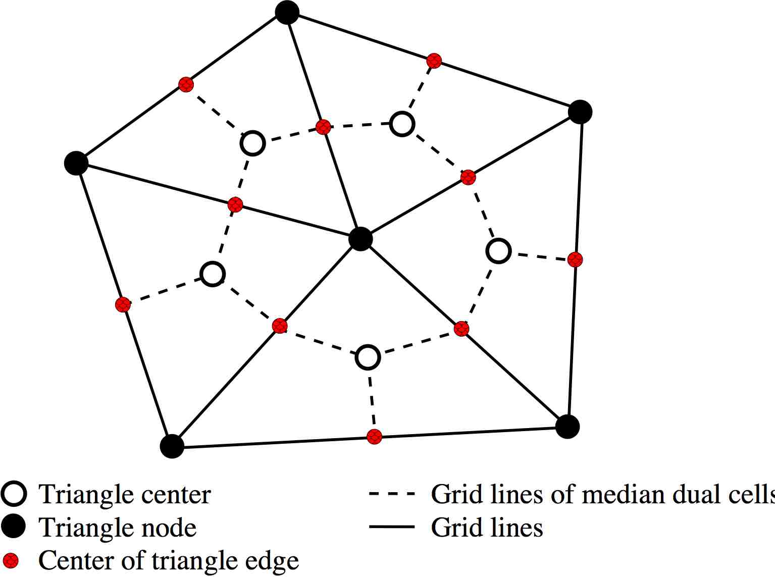
The first step in approximately solving (33) in some domain is to mesh the domain with a finite number of triangles. We will refer to this triangulation as , where refers to a representative triangle radius, which in this work we just take to be the square root of the triangle area: . Associated with this triangulation is a dual grid, which is constructed by connecting triangle centers to edge centers. A an example triangulation along with its dual grid is shown in Figure 1.
Unlike the discontinuous Galerkin approach [10, 22], approximate solutions are centered on triangle nodes (i.e., centers of the dual grid) rather than triangle centers. In order to obtain an update for these node centered values, we integrate (33) over the median dual cell and from to :
Next we define the median dual cell average and the time-averaged fluctuations through :
| (35) | ||||
| (36) |
Using these definitions, the update formula for a generic residual distribution scheme can be written as follows:
| (37) |
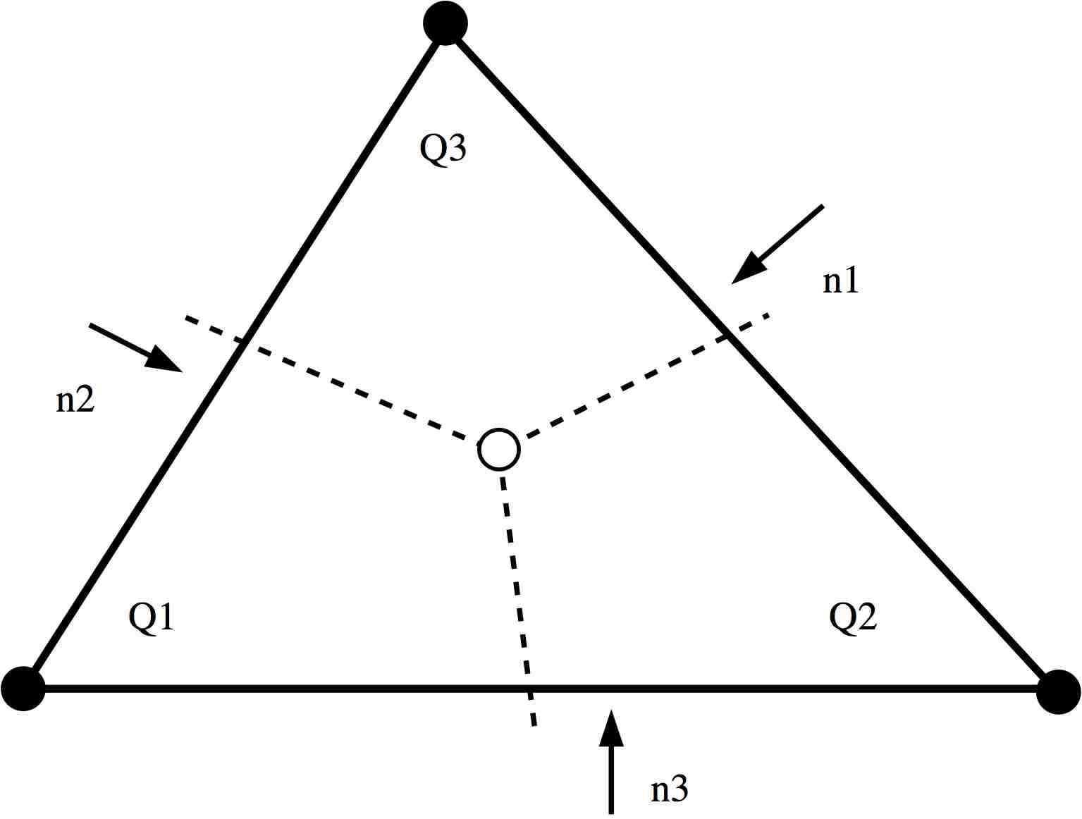
In the remainder of this work, we will approximate the exact solution, , with a piecewise constant representation, , that is constant on each median dual cell. We note that this view of RD schemes is slightly different than the standard view (e.g., [1]), where the approximate solution is usually viewed to be piecewise linear on each triangle . Although these descriptions seem contradictory, in the case for first-order accuracy in time, both interpretations yield the same numerical schemes. The advantage of viewing the solution as being piecewise constant on each medial dual cell is that this naturally sets up a series of multidimensional Riemann problems in each triangle (see Figure 2), which can be solved to construct the fluctuations111In this work, the terms distributed residual and fluctuation mean the same thing and are used interchangeably. . In this way, we can then view approximate constructions of as approximate Riemann solvers.
Computing the fluctuations is generally done using the following framework (again, the two interpretations, piecewise constant on each dual cell vs. piecewise linear on each primal cell, make use of the exactly the same framework):
-
1.
On each triangle construct a total residual:
(38) where denotes an interpolant that passes through the three nodal values
For example if we simply use linear interpolation, the total residual can be written as222For the standard N-scheme, which we will describe shortly, this is not the definition of the total residual that is used.
(39) Here represents the inward pointing normal vectors to the three edges of the triangle . The length of is equal to the length of the edge to which it is perpendicular. If the three nodes of triangle are given by for , then the three scaled normals can be written as
-
2.
Once this total residual has been calculated, it is then distributed to each of the nodes of the triangle:
The detailed strategy for how this distribution is accomplished yields a specific numerical method.
3.1 Design principles for scalar conservation laws
We first focus on design principles for scalar equations; in a subsequent subsection we explain how to extend this to the systems case. In order to obtain a numerical update that produces a stable and accurate approximation to (33), we will need the distribution strategy to satisfy certain properties:
-
1.
Numerical conservation: Since the interpolation of the numerical solution is continuous across triangle edges, conservation simply reduces to the following constraint:
(40) In other words, in a given triangle, the sum of the distributed residuals must equal the total residual.
-
2.
Monotonicity preserving: This condition makes sure that the numerical update satisfies a local maximum principle, which is needed to guarantee that the update does not generate any new spurious maxima or minima. If we write
(41) then the monotonicity requirement can be written as (see [13]):
(42) -
3.
Linear preserving: The order of accuracy of update (37) in the steady-state depends, among other things, on how accurately the total residual (38) is calculated on each triangle [6]. If we use formula (39), then in the steady state, which is the correct order of accuracy if want an approximate solution, , that is accurate in the steady state. What we actually need in order to get an accurate steady state solution is that not only that , but that each distributed residual also satisfies . The distributed residuals can be written as
(43) where measures the fraction of the total residual that is distributed to node . To ensure that the distributed residuals are of the same order as the total residual, we need to make sure that the ’s remain bounded as . Therefore, the accuracy condition, or more commonly referred to as the linear preserving condition, can be writtten as follows (see [13]):
(44)
3.2 Scalar N-scheme
Modern finite volume methods for hyperbolic PDEs are typically based on solving, either exactly or approximately, a Riemann problem between neighboring states. For multidimensional problems, a standard approach is to solve local 1D Riemann problems and then use the information from the Riemann solutions to construct numerical fluxes or fluctuations (see Chapters 19-21 of LeVeque [20]).
In the RD framework, however, a multidimensional Riemann problem is solved. In an arbitrary triangle , we consider the Riemann problem between three constant states: , , and (see Figure 2 for a depiction). Exact solutions to multidimensional Riemann problems are at best expensive to evaluate, and in general not well-understood for many hyperbolic systems such as the Euler equations from gas dynamics [25]. Therefore, in practice an approximate method such as the N-scheme (the “N” stands for Narrow) [12, 13] is utilized; this approach can be viewed as a multidimensional generalization of Roe’s approximate Riemann solver [23].
Just as in the 1D case, we define a Roe-average (henceforth called the Roe-Struijs-Deconinck average [12]):
| (45) |
where is an average of the three nodal values for on the current triangle . The Roe-Struijs-Deconinck average satisfies the following constraint, which generalizes the 1D constraint given by (29):
| (46) |
where is the linear interpolant passing through for . If the flux, , is at most a quadratic function of , then
| (47) |
The approximate Riemann solution gives rise to the following set of fluctuations:
| (48) |
where is the so-called upwind parameter. In 1D the the upwind parameter relative to state is always either if or if . In multidimensions, is obtained by enforcing the conservation constraint (40):
| (49) |
where we have made use of the following two identities:
In order to demonstrate that the N-scheme is monotonicity preserving, we rewrite (48) in the form (41) with
| (50) |
From this it can be shown that update (37) is monotone under the following CFL condition:
| (51) |
3.3 Linear preserving limiters
The N-scheme described so far is both conservative and monotonicity preserving; however, it is not yet linear preserving. The problem with the previously described N-scheme is that the weights (43) are not uniformly bounded independent of the mesh. In order to modify the N-scheme to achieve uniformly bounded ’s, Abgrall and Mezine [5] introduced a nonlinear limiting procedure. The limiting process takes the original and replaces them with limited versions, denoted . The simpler of the two approaches discussed in [5] yields the following formulas:
| (52) |
which guarantees that . The limited residuals are then given by
| (53) |
It is clear that this scheme is both linear preserving and conservative. Furthermore, Abgrall and Mezine [5] proved that the limited N-scheme retains the monotonicity properties of the original N-scheme with the same CFL condition (51).
3.4 Extension to systems
Following [12], the N-scheme is extended to systems of conservation laws by first defining the following averaged flux Jacobians:
| (54) |
where is a parameterization of and
| (55) |
In order to achieve a conservative linearization we must find a parameter vector, , such that the following constraint is satisfied:
| (56) |
where is the linear interpolant that passes through the points for and
| (57) |
As was shown in [12] (see also [1, 11]), constraint (56) will in general only be satisfied if we are able to find a parameterization, , such that the flux, , depends at most quadratically on each for . For the Euler equations from gas dynamics, as well as related systems, such a parameterization is known [12].
Assuming that a parameterization has been found, we proceed by diagonalizing the flux Jacobian:
where is the matrix of right eigenvectors and is the diagonal matrix of eigenvalues. Following the philosophy of Roe’s approximate Riemann solver [23], the systems N-scheme is obtained by applying the scalar N-scheme to each characteristic component. This results in the following method:
| (58) |
The upwind parameter can be recovered by enforcing local conservation:
| (59) |
Note that solving for involves inverting an matrix. Finally, we note that although it is based on a generalization of the monotone scalar N-scheme, the systems N-scheme is in general only approximately non-oscillatory for nonlinear systems of conservation laws. In practice, however, this scheme has been shown to work quite well for steady-state shock computations for systems such as the Euler equations from gas dynamics [1].
The systems N-scheme described so far is not linear preserving. In order that the limiting procedure developed for scalar equations can be re-used for systems, Abgrall and Mezine [5] proposed to project the distributed residuals into the eigenspace of the Roe-Struijs-Deconinck-averaged flux Jacobian in some direction . In practice, the direction is chosen from physical considerations. For example, in the case of the shallow water equations or the Euler equation from gas dynamics, an approach that gives good results in practice is to take to be the local Roe-Struijs-Deconinck-averaged fluid velocity: . Once a limiting direction has been chosen, the limiting procedure can be summarized as follows:
| end | ||
where and are the left and right eigenvectors of , respectively.
3.5 A correction for improved convergence
As was pointed out by Abgrall [2], the N-scheme in conjunction with the limiting procedure outlined in Section 3.4 has one major drawback: the method does not in general converge to a steady-state solution. The problem is not with the N-scheme itself, since this method does converge to a steady-state, but instead the problem lies in how the N-scheme interacts with the limiting procedure. In the same paper, Abgrall [2] also provided a cure for this problem. He arrived at the following distributed residual:
| (60) |
where , is the area of triangle , and is a grid and solution dependent parameter. Notice that conservation is not affected by this correction term. In order to produce a scheme that converges to a steady-state solution, needs to be chosen so that the correction is relatively small near shocks and relatively large in smooth regions . Abgrall [2] proposed the following formula:
| (61) |
where is the projection of onto some important eigen-direction. In the case of the compressible Euler equations, should be taken to be the projection of onto the entropy wave. In Section 5, in which we consider several numerical examples, we will refer to the limited and corrected N-scheme as the NLC-scheme.
4 Multidimensional relaxation systems
Having reviewed the relaxation scheme paradigm in Section 2 and residual distribution schemes in Section 3, we now turn to develop a multidimensional relaxation system framework. We again begin with the case of a scalar conservation law and introduce the following relaxation system:
| (62) |
where
| (63) | ||||
| (64) |
In these expressions, we assume that . Just as in the 1D case, we will separate the effects of the hyperbolic left-hand side of this equation from the relaxation source term on the right-hand side by by viewing (62) as being comprised of the following two sub-problems:
| (65) | |||
| (66) |
In subsequent discussion we will make use of the following matrix:
| (67) |
where such that . The three eigenvalues of are given by
| (68) | ||||
| (69) |
We note that these eigenvalues are strictly real.
Next we define a relaxation procedure that is analogous to the 1D case; the main difference is that in 2D a genuinely multidimensional Riemann problem such as the one depicted in Figure 2 must be solved. Instead of attempting to solve this exactly, we solve it with the standard N-scheme. The full procedure can then be summarized as follows:
-
1.
Choose values for the parameters , , , and .
-
2.
On an arbitrary triangle, , approximately solve the multidimensional Riemann problem associated with (65) by applying the standard N-scheme.
-
3.
Approximate the effect of equation (66) on the solution calculated in Step (2) by directly setting and . In other words, instantaneously relax the solution from Step (2) to the limit.
4.1 The N-scheme
The first scheme that we will produce with the relaxation procedure is the N-scheme applied to the original scalar conservation law. We set
| (70) |
where is the Roe-Struijs-Deconinck-average that satisfies (46). The above choice for and results in the following coefficient matrix for the relaxation system:
| (71) |
this matrix has eigenvalues given by
| (72) |
and, as in the 1D case, has an incomplete set of eigenvectors (i.e., the eigenvalues have algebraic multiplicity 3, but geometric multiplicity of only 2).
Because only has two linearly independent eigenvectors it cannot be diagonalized; and instead, we reduce it to Jordan canonical form via the following similarity transformation:
| (73) |
where
| (74) |
In approximately solving the Riemann problem via the N-scheme (Step (2) of the relaxation procedure), we will need to make sense of the expression . Without a full set of eigenvectors, we do this in the following way:
| (75) |
This results in two possibilities:
-
1.
;
-
2.
.
The first of these two expressions is exactly the result one should expect; the second expression, however, is somewhat troubling. We should expect that if , where
Instead, we are currently stuck with the following result when :
In order to clean up this result, we are forced to slightly modify the relaxation procedure for the N-scheme. We will leave the sub-problem (65) alone, but replace sub-problem (66) with the the following system of ODEs:
| (76) |
where is a piecewise constant function in space that is constant on each triangle ; the value of this constant is , the multidimensional Roe-Struijs-Deconinck average (46). This results in the following modification of Step (3) in the relaxation procedure:
-
3.
On each triangle approximate the effect of (76) on the solution calculated in Step (2) by directly setting and . In other words, instantaneously relax the solution from Step (2) to the limit.
Note that in general
and therefore, replacing (66) with (76) will yield a different numerical scheme. As we will demonstrate below, it is the scheme based on (76) that will reproduce the N-scheme.
The solution value at each node is now given by
| (77) |
Additionally, we enforce the condition:
| (78) |
With these modifications it is now true that if .
In order to proceed with the relaxation procedure, we solve a Riemann problem between three states of the form (77) with . Solving this Riemann problem via the N-scheme tells us that the residuals distributed to each node are given by
| (79) |
where has the form (78). In order to determine in terms of the values, we add the three residuals given by (79) and enforce that this sum yields the total residual in triangle :
| (80) | |||
| (81) |
If , then we note the following result on each triangle :
-
1.
,
-
2.
.
This result implies that there are two possibilities whenever : the 1-target case – exactly one s.t. , and the 2-target case – exactly two s.t. . Without loss of generality, let us assume that and , which yields one of the two possibilities:
| 1-target solution: | (82) | |||
| 2-target solution: | (83) |
We consider each of these two cases below.
4.1.1 The 1-target solution
The 1-target case is easy to analyze: the total residual is completely distributed to the lone node that is downwind of the flow, which we have taken without loss of generality to be node 1. If we let denote the component of the residual corresponding to , then the 1-target case results in the following residual distribution:
| (84) |
which is the same result that one would obtain with the N-scheme on the original scalar conservation law.
4.1.2 The 2-target solution
The 2-target case involves distribution to two nodes, which we have taken without loss of generality to be the 1 and 2 nodes. From equation (81) we arrive at the following linear system that must be solved in order to obtain the upwind parameter :
| (85) |
However, it is not difficult to show that
| (86) |
This implies that . Therefore the 2-target case results in the following residual distribution corresponding to Q:
| (87) |
This result is again identical to the original scalar conservation law.
4.2 The RXN-scheme: genuinely multidimensional local Lax-Friedrichs
One of the main difficulties with the N-scheme is that computing the upwind parameter for complicated systems of conservation laws can become prohibitively expensive. Despite this fact, few alternatives have been developed in the RD literature. One such alternative was introduced by Abgrall [2], who considered a local Lax-Friedrichs-type method that was obtained, in analogy to the 1D case, by taking the unstable “centered” residual and adding the appropriate numerical viscosity. In this work, we construct a new method based on the idea of relaxation systems; this scheme can be viewed as a different multidimensional generalization of the 1D LLF method. For brevity we will call this method the RXN-scheme, which stands for “relaxation N-scheme333the words “N-scheme” appear here because we make use of the N-scheme to solve the homogeneous part of the relaxation system..” In analogy with the 1D LLF method as derived in Section 2.3, we make the following choice for the parameters and in (62)–(64):
| (88) |
Note that each triangle can have a different value of ; this is why we call it a ‘local’ Lax-Friedrichs. This choice results in a coefficient matrix of the form
| (89) |
which has an eigenvector decomposition given by
| (90) |
The Chapman-Enskog expansion for this relaxation system can be written to first order as
| (91) |
The eigenvalues of the diffusion matrix in the above expression are
| (92) |
which results in the following restriction on the choice of the lone parameter :
| (93) |
for all .
Applying the N-scheme to the relaxation system with coefficient matrix (89), yields the following residual
| (94) |
where . Simplifying this expression gives
| (95) |
In order to calculate , we must enforce conservation:
| (96) |
which results in the following linear system for the upwind parameters :
| (97) |
The solution to this linear system can be written as
| (98) | ||||
| (99) | ||||
| (100) |
where
| (101) |
Let us now take a moment to reflect on what just happened. Although the original coefficient matrix, (89), for this method was comically simple, after applying the N-scheme to this system on an arbitrary triangle, the resulting upwind parameters are somewhat complicated. On the other hand, we see from equation (97) that the parameter is completely decoupled from . We make use of this last fact to construct an alternative scheme in the following way: instead of computing the components of from (99)–(101), we enforce
| (102) |
by again invoking the relaxation limit. Although this direct enforcement clearly gives a different scheme than if we had used (99)–(101), what we achieve with this approach is a very simple method that we refer to as the RXN-scheme (relaxation N-scheme). In terms of the residual distributed to node in the -variable, we now obtain the following expression:
| (103) |
where is given by (98). Note that this method is automatically conservative since still satisfies the first equation in linear system (97).
Theorem 4.1
(Monotonicity) If there exists a such that
| (104) |
and
| (105) |
where for each
| (106) |
from the Rankine-Hugoniot conditions, then the RXN-scheme as defined by (103) and (98) satisfies the following condition:
| (107) |
where for all . This condition along with the following CFL constraint on the time step:
| (108) |
is enough to guarantee that the RXN-scheme with forward Euler time-stepping (37) is monotonicity preserving.
-
Proof.
(1) Using the Rankine-Hugoniot conditions (106), we rewrite the RXN-scheme as
(109) Similarly, we rewrite (98) as follows
(110) Note that the above expression was obtained by making use of (104) and the identity: . Combining expressions (109) and (110) yields (107) with
(111) We note that , because (105) implies that and .
4.3 Systems N-scheme
The systems generalization of coefficient matrix (89) for a system of conserved variables is the following matrix:
| (112) |
where is again the identity matrix, is the matrix with zeros in every entry, and is the flux Jacobian matrix evaluated at the Roe-Struijs-Deconinck average [12]. The systems generalization of (77)–(78) are the following vectors:
| (113) |
In order to calculate the appropriate residuals in the relaxation procedure, we need to again understand how to create the matrices and . As in the scalar case this is complicated by the fact that does not have a full set of eigenvectors. In particular, the Jordan canonical form of this matrix can be written as
| (114) |
Here is the eigenvalue of the matrix . We omit the complicated expression for the matrix . In order to obtain an expression for , one has to replace each in the above expression with . Carrying this out results in the following matrix:
| (115) |
where , is the diagonal matrix of eigenvalues of , and is the corresponding matrix right-eigenvectors. An analogous formula for can also be readily constructed. From the above expression we find that
| (116) |
Having established expressions for , we now proceed by applying the N-scheme to the relaxation system:
| (117) |
where
| (118) |
and . The unique solution to the linear system in (117) is with
| (119) |
and the component of the residual associated with can be written as
| (120) |
This result shows that this relaxation scheme identically reproduces the systems N-scheme (58)–(59).
4.4 Systems RXN-scheme
Just as the LLF method in the one-dimensional case, the RXN-scheme extends to systems of conservation laws in a simple manner. All that we have to do is apply the scalar version of the scheme to each component of the vector conserved variable. The coefficient matrix in the relaxation procedure can be written as
| (121) |
where is the identity matrix. In order to satisfy the sub-characteristic condition we require that
| (122) |
over all . In the above expression and are the eigenvalue of and , respectively.
We note that the systems RXN-scheme, and in particular, the version of this scheme with limiters (Section 3.4) and convergence corrections (Section 3.5), provides an alternative to the systems N-scheme that does not require the inversion of an matrix in each element at each time level, nor does it require any special entropy fixes or special treatment near stagnation points. Since this method is also simpler than the N-scheme, it should also yield some gains in computational efficiency. The systems N-scheme and RXN-scheme are compared in detail in Section 5.
4.5 RXN-scheme in -dimensions
The above procedure for obtaining the 2D RXN-scheme can be generalized to any space dimension. In the -dimensional case we arrive at the following scheme:
| (123) |
where
| (124) |
In particular, we note that for , this scheme exactly reduces to the 1D local Lax-Friedrichs method [24]. We also mote that the geometric factor comes from the -dimensional N-scheme; see for example equation (7) in [11].
5 Numerical examples
In this section we compare the N-scheme and the newly proposed RXN scheme on several numerical examples. We will refer to the versions of the N-scheme and RXN-scheme that have been limited according to the procedure outlined in Section 3.4 and corrected according to the procedure outlined in Section 3.5 as the NLC-scheme and RXNLC-scheme, respectively.
5.1 Steady-state advection
First, we consider the advection equation on :
| (125) |
with non-divergent velocity and boundary conditions given by
This same problem was considered in [2].
For a non-divergent velocity field, an elegant way to solve the advection equation using the N-scheme is through the introduction of a streamfunction:
such that . The N-scheme can then be written as
where
The advantage of this formulation is that we achieve numerical conservation, even though the equations are solved in advective form.
For the RXN scheme, we use residual (103) where the flux functions are given by
and is given by (97) as usual.
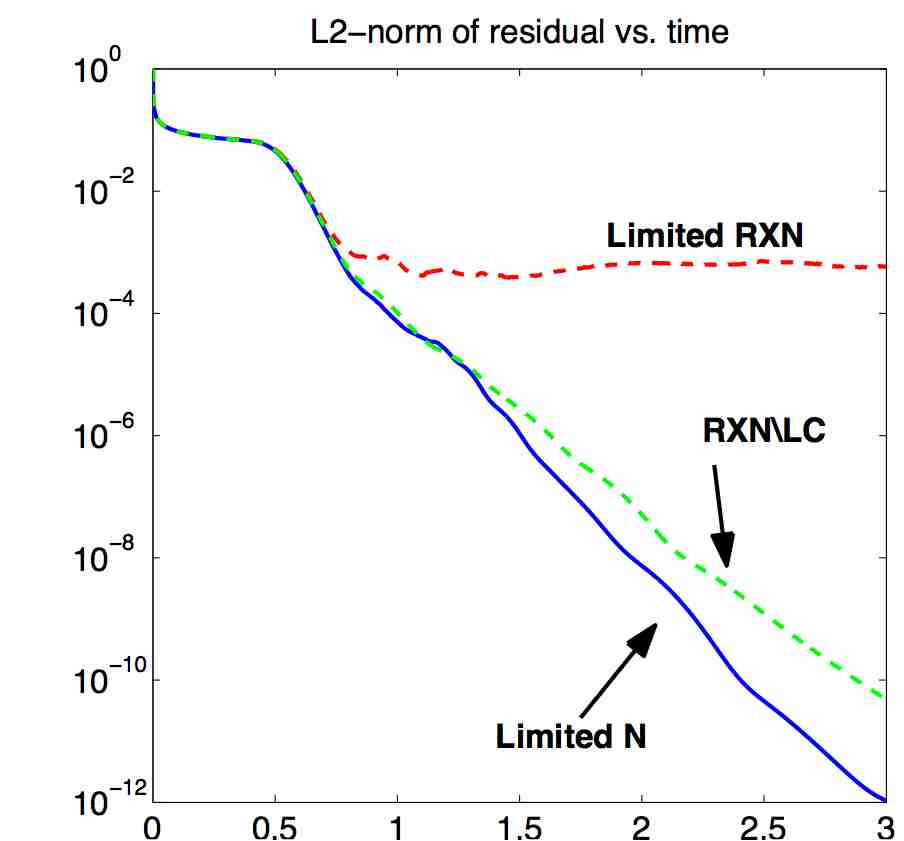
Results on a grid with 5592 elements and 2903 nodes is shown in Figure 3; displayed in each panel are (a) the basic N-scheme, (b) the basic RXN-scheme, (c) the limited N-scheme (no convergence correction is needed for the limited N-scheme on scalar equations), and (d) the RXNLC-scheme (convergence corrections are needed for the limited RXN-scheme, even for scalar problems). These results show that the basic RXN scheme is far more diffusive than the N-scheme. However, with limiting and convergence corrections, the RXNLC-scheme gives results comparable to the limited N-scheme. Convergence histories for the limited N-scheme, limited RXN-scheme, and the RXNLC-scheme are shown in Figure 4.
Clearly there is no advantage in using the RXNLC-scheme over the limited N-scheme for a scalar problem, since the two methods have the same computational cost and the scalar limited N-scheme does not require convergence corrections. However, for hyperbolic systems such as the Euler equations, the RXNLC-scheme provides a simpler algorithm with lower computational cost than the NLC-scheme.
5.2 Transonic flow around the NACA 0012 airfoil
Next we consider transonic flow around the NACA 0012 airfoil using the compressible Euler equations from gas dynamics as our model. The Euler equations can be written as
| (126) |
where is the fluid density, is the fluid velocity, is the total energy, and is the fluid pressure. The ideal gas law closes the system by relating the pressure to the other fluid variables:
| (127) |
where is the ideal gas constant. In this example we take .
The computational domain and numerical grid is shown in Figure 5(a). In Figure 5(b), we show a zoomed-in view of the numerical grid near the airfoil. The boundary conditions are such that subsonic flow with Mach number 0.85 enters from the left boundary at an angle of from the horizontal axis. As the flow impinges on the airfoil, two supersonic bubbles are created above and below the airfoil. The supersonic flow is decelerated to the ambient subsonic flow through the creation of two shock waves (again, one above the airfoil and one below). This problem has been considered in several papers including [1, 2].
Isolines of the Mach number and the pressure are shown in Figure 6. We also plot in Figure 7 the Mach number along the top and bottom edges of the airfoil. From this figure we note that the location of the shocks is in very good agreement between the two methods, while the location at the front of the airfoil where the solution goes from subsonic to supersonic is slightly different for each method. Furthermore, the RXNLC-scheme is more diffusive than the NLC-scheme, which results in slightly more entropy production near the airfoil for RXNLC than NLC. This can be seen both in Figure 6, where we see bending of the Mach isolines near the airfoil, as well as in Figure 8. Overall, however, both of these figures indicate remarkable agreement between the two solutions. In particular, the RXNLC solution is far closer to the NLC solution than the MUSCL-type scheme that was presented in [1]. We also note that the RXNLC-scheme runs twice as fast as the NLC-scheme.
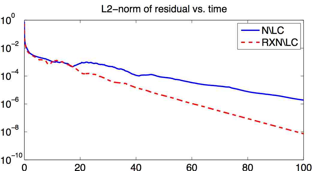
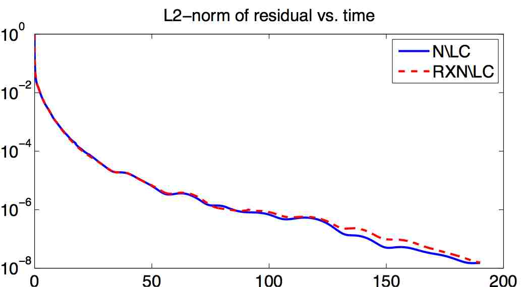
Finally, in Figure 9 we show the -norm of the total residual as a function of time. We note that the fix of Abgrall [2] (see Section 3.5) is critically important in bringing both methods to convergence. Without this fix both methods stall at a total residual of only about . We also find that the RXNLC-scheme has a slightly better convergence rate than the NLC-scheme.
5.3 Supersonic flow around a cylinder
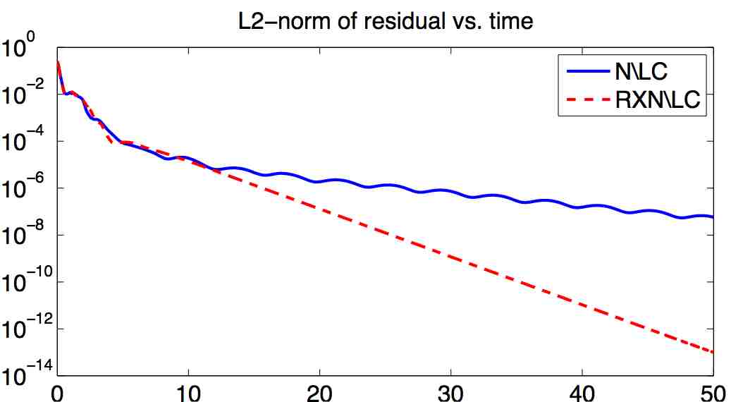
Next we consider flow around a cylinder with Mach number . The computational domain is with a cylinder of unit radius centered at . In this example we found that we needed to run all the schemes at a CFL number of 0.4 in order to obtain well-converged results. The steady-state pressure on a grid with 5144 elements and 2656 nodes is shown in Figure 10 for the following schemes: (a) the basic N-scheme, (b) the basic RXN-scheme, (c) the NLC-scheme, and (d) the RXNLC-scheme. The basic RXN-scheme solution is far more diffusive than the basic N-scheme, but once limiters and the convergence corrections are added, the NLC and RXNLC schemes produce comparable results. In fact, the RXNLC-scheme converges faster than the NLC-scheme, as can be seen in the convergence plot in Figure 11. Finally, we note that the RXNLC-scheme again runs about twice as fast as the NLC-scheme.
5.4 Subsonic flow around a cylinder
Finally, we consider flow around a cylinder with Mach number . This problem has been considered in several papers including [1, 2]. The computational domain is with a cylinder of radius centered at . The steady-state Mach number on a grid with 12552 elements and 6404 nodes is shown in Figure 12 for the (a) NLC and (b) RXNLC schemes. Near the cylinder both methods produce comparable results. Away from the cylinder the grid resolution becomes coarser; and therefore, visible differences in the two methods appear. In these regions the RXNLC scheme produces slightly more diffused contours than the NLC scheme.
Shown in Figure 13 are the deviation of the physical entropy, , from the ambient entropy, : . Panel (a) is the NLC-scheme and panel (b) is the RXNLC-scheme. The minimum and maximum values of for the NLC and the RXNLC schemes are and , respectively. Each panel consists of 31 contour lines ranging from the minimum to the maximum for each scheme. Therefore, these results show that the RXNLC-scheme has a smaller entropy deviations, but that this error is more spread out behind the cylinder, while the NLC-scheme has larger entropy deviations, but that this error is more concentrated near the -axis.
The total residual as a function of time is shown in Figure 14. Both methods give essentially the same convergence rates for this example. Finally, we note that the RXNLC-scheme again runs about twice as fast as the NLC-scheme.
6 Conclusions
In this work we have extended the results of LeVeque and Pelanti [21] to genuinely multidimensional residual distribution schemes. Specifically, we have shown that the N-scheme, both the scalar and the systems version, can be derived from a relaxation principle. Furthermore, using a genuinely multidimensional extension of the 1D local Lax-Friedrichs relaxation principle, we have derived a novel residual distribution scheme. The main benefit of this approach is that it does not require the inversion of an matrix, where is the number of conserved variables, at each time step in each grid element. The new method also does not require the use of Roe-Struijs-Deconinck averages. Using several examples of the 2D Euler equations from gas dynamics, including an example of transonic flow around the NACA 0012 airfoil, supersonic flow around a cylinder, and subsonic flow around a cylinder, we have compared the limited and corrected N-scheme (NLC) with the newly proposed scheme (RXNLC). These comparisons show that despite being computationally less expensive, the new method is capable of producing results comparable to those of the NLC-scheme, although often with slightly more numerical diffusion. For more complicated equations such as magnetohydrodynamics or the general relativistic Einstein equations, we believe that the benefit of a simpler and computationally less expensive algorithm will far outweigh the slight increase in numerical dissipation. We will consider some of these more complicated systems in future work.
Finally, we would like to point out that the numerical code used in this work, including all of the numerical grids, will be made publicly available as part of the REDPACK software project. For more information see
Acknowledgements. The author would like to thank the two anonymous reviewers for their very helpful comments. This work was supported in part by NSF grants DMS–0619037 and DMS–0711885.
(a) 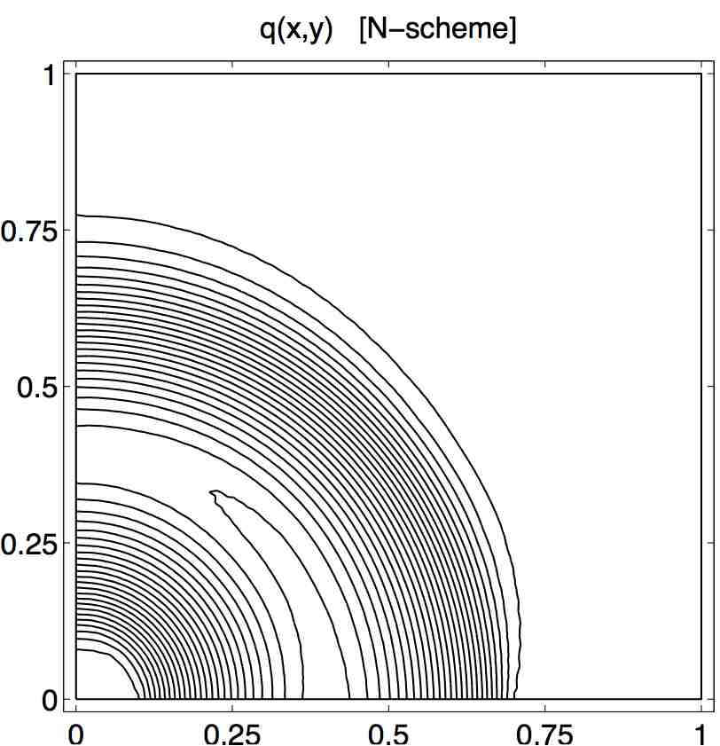 (b)
(b) 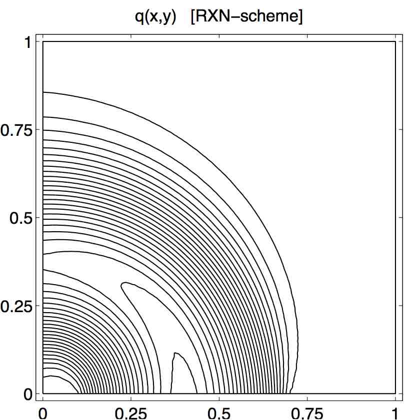
(c) 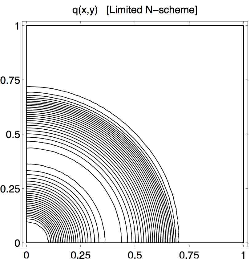 (d)
(d) 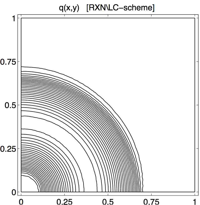
(a) 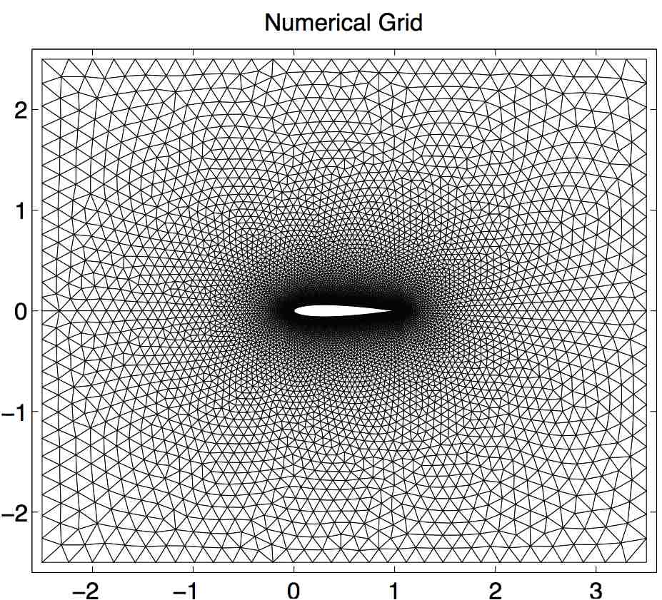 (b)
(b)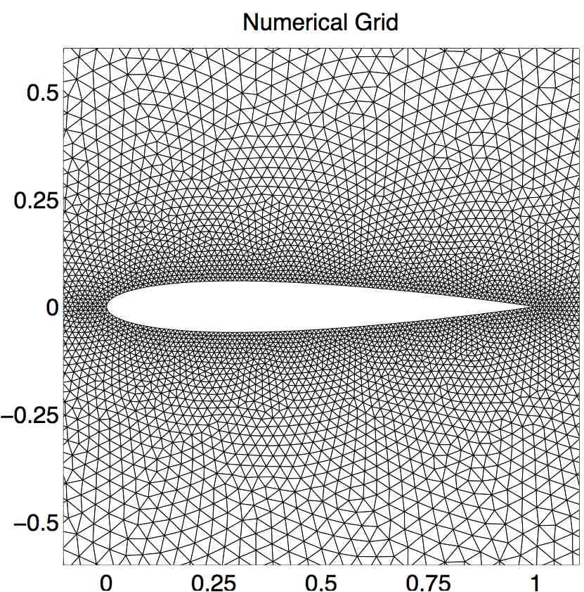
(a) 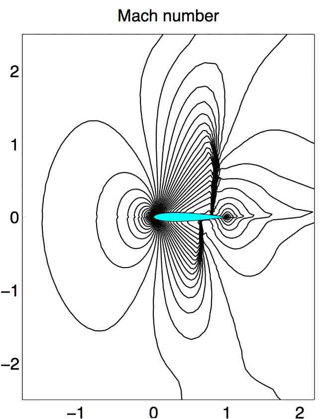 (b)
(b)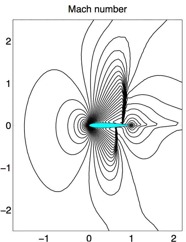
(c) 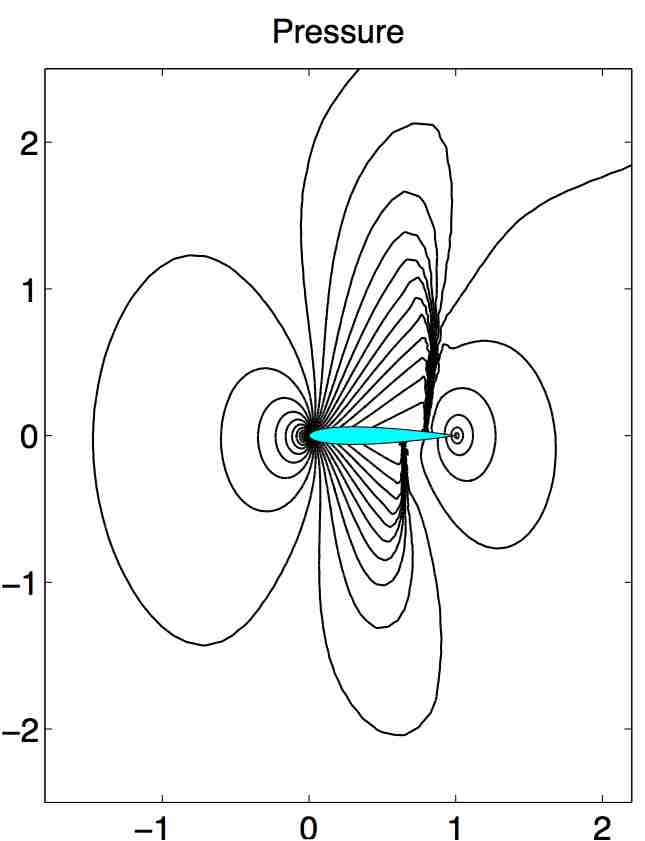 (d)
(d)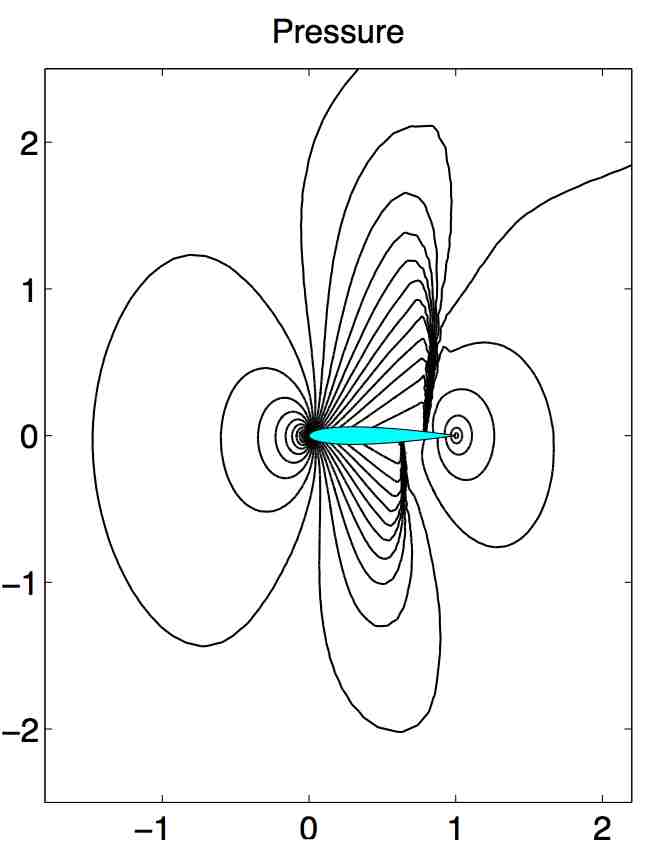
(a) 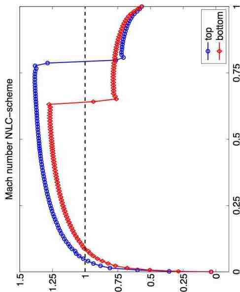 (b)
(b)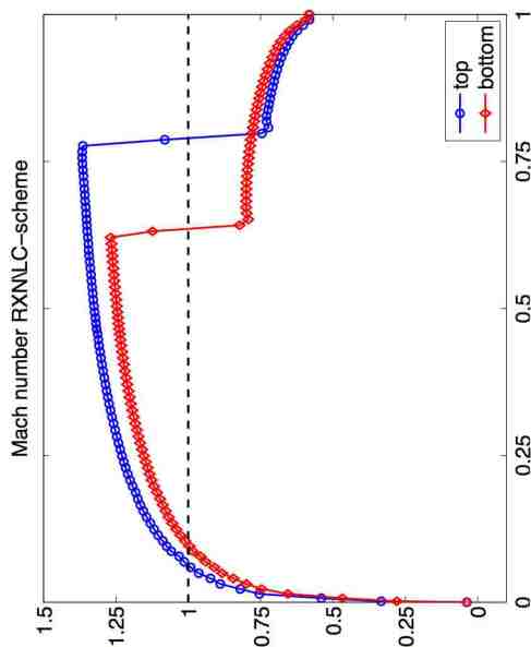
(c) 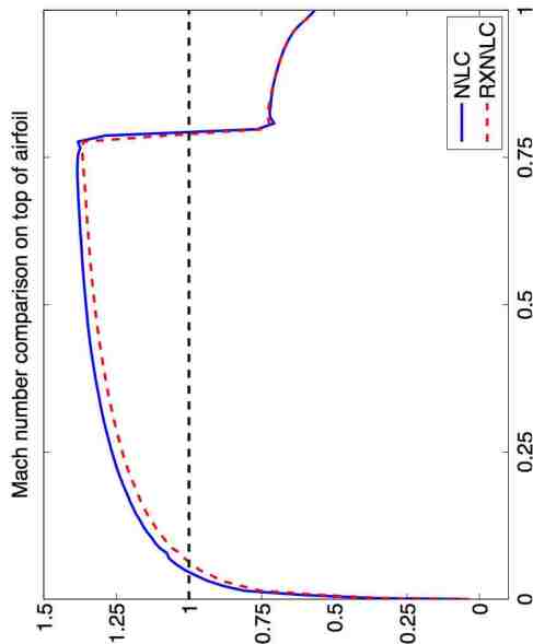 (d)
(d)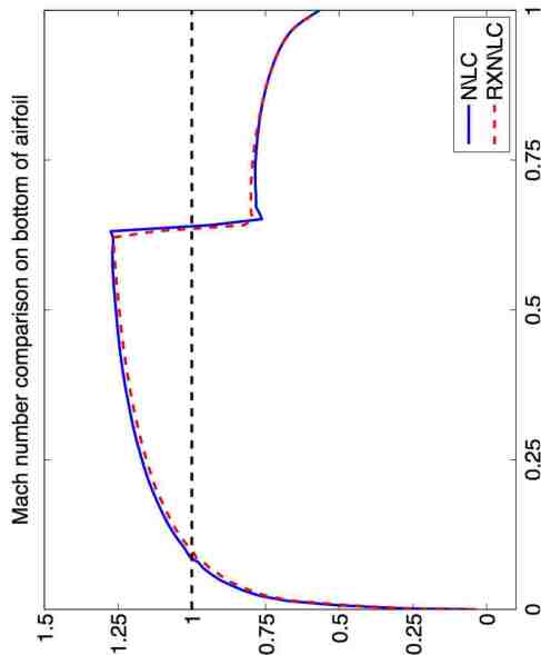
(a) 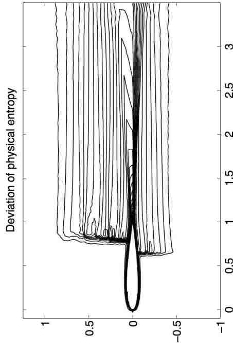 (b)
(b) 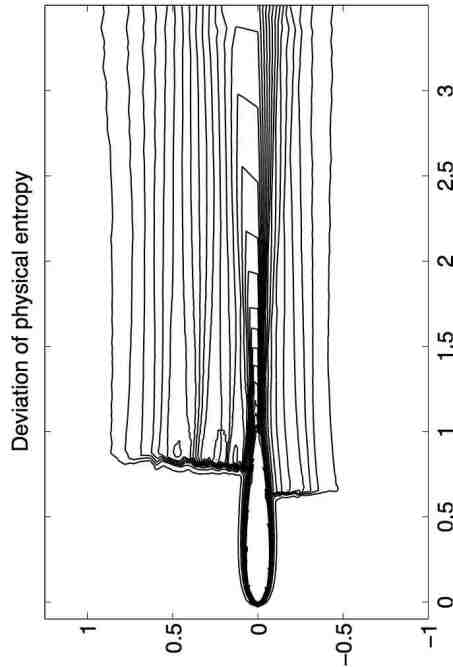
(a) 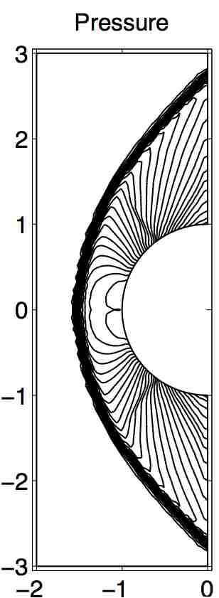 (b)
(b) 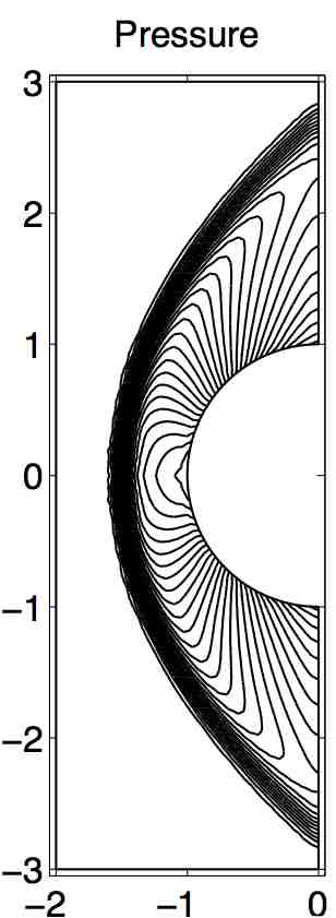
(c) 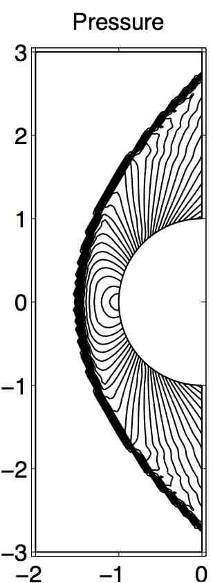 (d)
(d) 
(a) 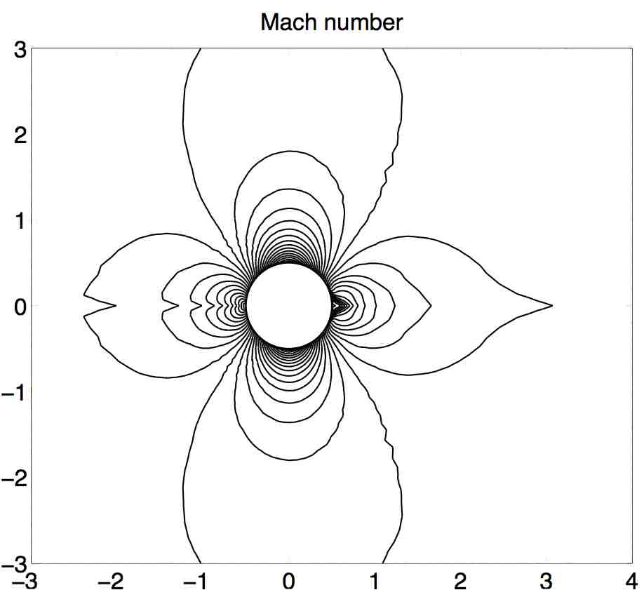
(b) 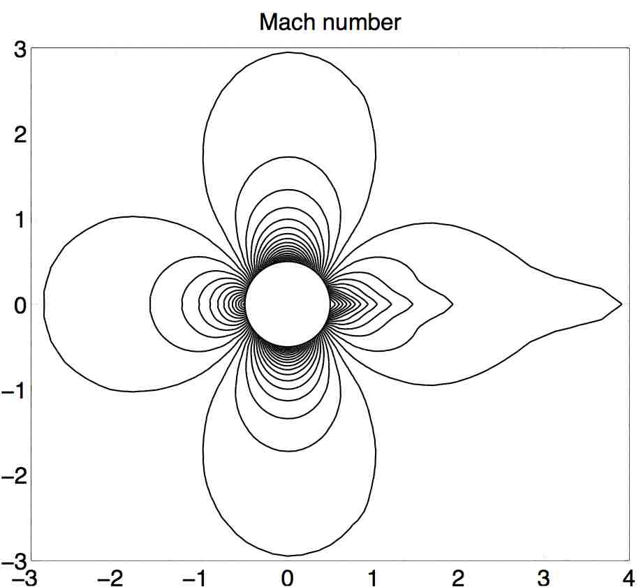
(a) 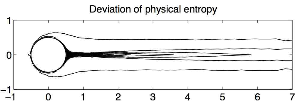
(b) 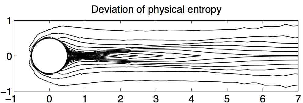
References
- [1] R. Abgrall. Toward the ultimate conservative scheme: Following the quest. J. Comp. Phys., 167:277–315, 2001.
- [2] R. Abgrall. Essentially non-oscillatory residual distribution schemes for hyperbolic problems. J. Comp. Phys., 214:773–808, 2006.
- [3] R. Abgrall. Residual distribution schemes: Current status and future trends. Comput. Fluids, 35:641–669, 2006.
- [4] R. Abgrall and M. Mezine. Construction of second order accurate monotone and stable residual distribution schemes for unsteady problems. J. Comp. Phys., 188:16–55, 2003.
- [5] R. Abgrall and M. Mezine. Construction of second-order accurate monotone and stable residual distribution schemes for steady problems. J. Comp. Phys., 195:474–507, 2004.
- [6] R. Abgrall and P.L. Roe. High order fluctuation schemes on triangular meshes. J. Sci. Comp., 19:3–36, 2003.
- [7] F. Bouchut. Nonlinear Stability of Finite Volume Methods for Hyperbolic Conservation Laws and Well-Balanced Schemes for Sources. Birkhuser Verlag, 2005.
- [8] G.Q. Chen, C.D. Levermore, and T.P. Liu. Hyperbolic conservation-laws with stiff relaxation terms and entropy. Comm. Pure Appl. Math., 47:787–830, 1994.
- [9] G. Chesshire and W.D. Henshaw. Composite overlapping meshes for the solution of partial-differential equations. J. Comp. Phys., 90:1–64, 1990.
- [10] B. Cockburn and C.-W. Shu. The Runge-Kutta discontinuous Galerkin method for conservation laws V: Multidimensional systems. J. Comp. Phys., 141:199–224, 1998.
- [11] Á. Csík, M. Ricchiuto, and H. Deconinck. A conservative formulation of the multidimensional upwind residual distribution schemes for general nonlinear conservation laws. J. Comp. Phys., 179:286–312, 2002.
- [12] H. Deconinck, P.L. Roe, and R. Struijs. A multidimensional generalization of Roe’s difference splitter for the Euler equations. Comput. Fluids, 22:215–222, 1993.
- [13] H. Deconinck, G. Struijs, G. Bourgeois, and P. Roe. Compact advection schemes on unstructured meshes. In VKI Lecture Series 1993-04, Computational Fluid Dynamics, 1993.
- [14] A. Harten, P.D. Lax, and B. van Leer. On upstream differencing and godunov-type schemes for hyperbolic conservation laws. SIAM Review, 25:35–61, 1983.
- [15] C. Helzel. A high-resolution rotated grid method for conservation laws with embedded geometries. SIAM J. Sci. Comput., 26:785–809, 2005.
- [16] G.S. Jiang and C.-W. Shu. Efficient implementation of weighted eno schemes. J. Comp. Phys., 126:202–228, 1996.
- [17] S. Jin and Z.P. Xin. Relaxation schemes for systems of conservation-laws in arbitrary space dimensions. Comm. Pure Appl. Math., 48:235–276, 1995.
- [18] A. Kurganov and E. Tadmor. New high-resolution central schemes for nonlinear conservation laws and convection-diffusion equations. J. Comp. Phys., 160:241–282, 2000.
- [19] R.J. LeVeque. Wave propagation algorithms for multi-dimensional hyperbolic systems. J. Comp. Phys., 131:327–335, 1997.
- [20] R.J. LeVeque. Finite Volume Methods for Hyperbolic Problems. Cambridge University Press, 2002.
- [21] R.J. LeVeque and M. Pelanti. A class of approximate Riemann solvers and their relation to relaxation schemes. J. Comp. Phys., 172:572–591, 2001.
- [22] W.H. Reed and T.R. Hill. Triangular mesh methods for the neutron transport equation. Technical Report LA-UR-73-479, Los Alamos Scientific Laboratory, 1973.
- [23] P.L. Roe. Approximate Riemann solvers, parameter vectors, and difference schemes. J. Comp. Phys., 43:357–372, 1981.
- [24] V.V. Rusanov. Calculation of interaction of non-steady shock waves with obstacles. J. Comp. Math. Phys. USSR, 1:267–279, 1961.
- [25] C.W. Schulzrinne, J.P. Collins, and H.M. Glaz. Numerical-solution of the Riemann problem for 2-dimensional gas-dynamics. SIAM J. Sci. Comput., 14:1394–1414, 1993.
- [26] E. van der Weide and H. Deconinck. Positive matrix distribution schemes for hyperbolic systems. In Computational Fluid Dynamics 1996, pages 747—753. Wiley, 1996.
- [27] B. van Leer. Towards the ultimate conservative difference scheme V. A second order sequel to Godunov’s method. J. Comp. Phys., 32:101–136, 1979.