Coherence Induced by Incoherent Pumping Field and Decay Process in Three-level $\Lambda$ Type Atomic System

Abstract

Following the method of Victor V. Kozlov et al.[PhysRevA. 74. 063829],we inspect the atomic coherence induced by incoherent pump and spontaneous decay process in $\Lambda$ type three-level atomic system with degenerated lower duplicate levels. The system shows a coherent population trapping state and multi-steady states characteristic in different conditions. Interestingly, we derived two kinds of different steady states generated by the system in different sets of pumping and decaying parameters, the ”robust” steady state and the ”weak” steady state, which exhibit stable or unstable characteristics under the action of pump field and vacuum reservoir. These two kinds of steady states help to understand the coherence excitation mechanism, and will promise fruitful applications to atomic coherence and interference in quantum optics.

I Introduction

Quantum coherence effects such as coherent population trapping(CPT)CPT , electromagnetically induced transparency(EIT)EIT , lasering without inversion(LWI)LWI LWI2 and etc, are extensively studied in quantum opticsQuantOpt QuantOpt2 . However most of the study on atomic coherent effect focus on coherent process as the coherent pump procedure, the possibility of atomic coherence induced by incoherenct process was not recognized until late in the middle of last decadeZhu95 . Since then, a lot of new schemes on application of coherent effect based on the incoherent character of atomic system are proposed , for example, quenching spontaneous emissionQuenchSp QuenchSp2 , lasing without inversionPRA063829 and so on. In fact the coherent process as the coherent pump is not a unique condition to produce the upper quantum coherent effects. For instance, in the V type three level system, coherence can be produced by incoherent process, i.e., the decay process and incoherent pumpPRA063829 .

Following the method proposed in the Victor V. Kozlov’s paperPRA063829 , we discuss a different situation, the $\Lambda$ type three level system. Here the $\Lambda$ system also shows coherent population trapping feature and the multi-steady state character. And we find out an interesting phenomenon that in the coherent population trapping state, levels population are only related to the incoherent pumping rates, totally unrelated to the decay rate, which is different from the situation in the $V$ type system, where the pumping and decay rates are relevant. Thus we can adjust the proper pumping rate parameter to change the level population from almost zero population state to nearly full population state or vice versa, which is similar to the coherent pumping three-level $\Lambda$ system to CPT stateQuantOpt . What’s more interesting is that under one special set of pumping parameters, we produce a ”robust” steady state, which remains its original form under the interaction of pumping field and decaying process.

In this paper we also inspect the population transferring picture and atomic coherence excitation mechanism in detail, and find that coherence is produced by the destructive interference of incoherent pump process and decay process. Under specific conditions, the decay process can be totally suppressed by incoherent pump process, as a result, the ”robust” steady state is produced. On the other hand, when the pumping field is switched off, coherence can also be generated by spontaneous emission decay procedure, and the final state of atomic system comes to the ”weak” steady state, which shows unstable property under nonvanishing pump driving condition. The peculiar nature of the $\Lambda$ type three-level atomic system will promise fruitful applications in quantum optics.

This paper is organized as follows: in Sec.II, we derive the motion equations for density-matrix of the three level $\Lambda$ atomic system. In Sec.III, we derive solutions to the atomic motion equations under two kind of conditions, the general steady state situation in Sec.III.1 and the specific initial conditions in Sec.III.2, where the interesting character of the atomic system will be revealed. Finally in Sec.IV we discuss the potential applications for the system and set our conclusion.

II Master Equation of Three Level $\Lambda$ Atomic system

We are discussing a $\Lambda$ type three level atomic system shown in Fig.1, where the upper state $|a\rangle$ is connected to two lower closely spaced states $|b\rangle$ and $|c\rangle$ by dipole-allowed transition. The incoherent pump field $R$ drives the two lower states to the same upper state and back. The upper state decays through two different paths to lower states.

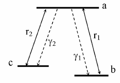
Figure 1: Scheme of a three-level $\Lambda$ type atomic system with closely doublet lower levels. $r_{1}$and $r_{2}$ are incoherent pump rates; $\gamma_{1}$ and $\gamma_{2}$ are decay rates.

Firstly we will derive the motion equations of the density-matrix elements for the atomic system. The interaction hamiltonian of the system in the interaction picture is shown in Eq.(1):

$$H=V_{\gamma}+V_{R}.$$ (1)

The first term on the right side of Eq.(1), $V_{\gamma}$ is the interaction with the reservoir of vacuum oscillators. The specified hamiltonian of this term reads as Eq.(2).

$$V_{\gamma}=\hbar\sum_{k}[g_{k1}a_{k}^{{\dagger}}|b\rangle\langle{a}|e^{-i\Delta_{k1}t}+g_{k1}^{*}a_{k}|a\rangle\langle{b}e^{i\Delta_{k1}t}$$

$$+g_{k2}a_{k}^{{\dagger}}|b\rangle\langle{c}|e^{-i\Delta_{k2}t}+g_{k2}^{*}a_{k}|c\rangle\langle{b}e^{i\Delta_{k2}t}],$$ (2)

where $g_{k1,k2}$ are the coupling constants between the kth vacuum mode and the atomic transitions from level $|a\rangle$ to level $|b\rangle$ (from level $|a\rangle$ to level $|c\rangle$). Without losing the generality, we take the coupling constants $g_{k1,k2}$ the real numbers. The detunings $\Delta_{k1}=\omega_{ab}-\nu_{k},\Delta_{k2}=\omega_{ac}-\nu_{k}$ are the difference between transitions frequencies $\omega_{ab}$, $\omega_{ac}$ and the vacuum mode $\nu_{k}$. And $\hat{a}_{k}$$(\hat{a}^{{\dagger}}_{k})$ is the annihilation(creation) operator of a photon in the kth vacuum mode, which obey the bosonic commutation rule: $[\hat{a}_{k},\hat{a}^{{\dagger}}_{k^{\prime}}]=\delta_{kk^{\prime}}$.

Another incoherent process in Fig.1 is the incoherent pumping process, which is described in the second term $V_{R}$ on the right side of Eq.(1), the specified hamiltonian of incoherent field $R$ takes the following form of Eq.(3):

$$V_{R}=\mu_{ba}R^{*}\sigma_{1}^{-}+\mu_{ab}R\sigma_{1}^{{\dagger}}+\mu_{ca}R^{*}\sigma_{2}^{-}+\mu_{ac}R\sigma_{2}^{{\dagger}},$$ (3)

where the dipole matrix elements $\mu_{ab}$ and $\mu_{ac}$ are the coupling constants for the incoherent field $R$ coupling with the atomic system. The following relationship shows the incoherent feature of the pumping field $R$:

$$\langle R^{*}(t)R(t^{\prime})\rangle=\mathcal{R}\delta(t-t^{\prime}).$$ (4)

The Liouville equation for the atomic system, incoherent pumping field and vacuum reservoir is:

$$\dot{\rho}_{T}=-\frac{i}{\hbar}[H,\rho],$$ (5)

where $\rho_{T}$ is the density operator for total system of the atom, pumping field and vacuum reservoir, and the hamiltonian H consists of the vacuum induced decaying part and the incoherent pumping part. We first formally integrate the Eq.(5), and then substitute it back to the Eq.(5), neglecting terms higher than second order:

$${\dot{\rho}}_{T}=-\frac{i}{\hbar}[H(t),\rho_{T}(0)]-\frac{1}{{\hbar}^{2}}\int^{t}_{0}[H(t),[H(t^{\prime}),\rho_{T}(t^{\prime})]]dt^{\prime},$$ (6)

where $t=0$ is chosen as the initial time. Note that the hamiltonian $H$ contains two separated processes, the decaying one and the pumping one, we can treat them independently in the upper Eq.(6), and then joint them together to get the motion equation for the concerned atomic system. Take the decaying part one for instance, we take the routine Weisskopf-Wigner approximation, assuming that the reservoir is large enough and the couple to the atomic system is very weak, then the density operator $\rho_{T}$ for the total system can be factorized into direct product of the atomic density operator $\rho$ and the density operator of reservoir $\rho_{r}$ at all time: $\rho_{T}=\rho\otimes\rho_{r}$. With this assumption, the motion equation for the atomic system is:

$$\dot{\rho}=Tr_{R}[\dot{\rho}_{T}]=-\frac{i}{\hbar}Tr_{R}[H(t),\rho_{T}(0)]$$

$$-\frac{1}{{\hbar}^{2}}Tr_{R}\int^{t}_{0}[H(t),[H(t^{\prime}),\rho_{T}(t^{\prime})]]dt^{\prime},$$ (7)

where $Tr_{R}$ denotes trace over the vacuum reservoir.

After long and complex calculation, we obtain the following set of equations for the atomic density matrix elementsQuantOpt PRA063829 :

$$\dot{\rho}_{aa}=-(\gamma_{1}+\gamma_{2}+r_{1}+r_{2})\rho_{aa}+r_{1}\rho_{bb}+r_{2}\rho_{cc}$$

$$+p\sqrt{r_{1}r_{2}}(\rho_{bc}+\rho_{cb})$$ (8)

$$\dot{\rho}_{cc}=\gamma_{2}\rho_{aa}+r_{2}(\rho_{aa}-\rho_{cc})-\frac{1}{2}p\sqrt{r_{1}r_{2}}(\rho_{bc}+\rho_{cb})$$ (9)

$$\dot{\rho}_{bb}=\gamma_{1}\rho_{aa}+r_{1}(\rho_{aa}-\rho_{bb})-\frac{1}{2}p\sqrt{r_{1}r_{2}}(\rho_{bc}+\rho_{cb})$$ (10)

$$\rho_{aa}+\rho_{bb}+\rho_{cc}=1$$ (11)

$$\dot{\rho}_{ab}=-\frac{1}{2}(\gamma_{1}+\gamma_{2}+2r_{1}+r_{2})\rho_{ab}-\frac{1}{2}p\sqrt{r_{1}r_{2}}\rho_{ac}$$ (12)

$$\dot{\rho}_{ac}=-\frac{1}{2}(\gamma_{1}+\gamma_{2}+r_{1}+2r_{2})\rho_{ac}-\frac{1}{2}p\sqrt{r_{1}r_{2}}\rho_{ab}$$ (13)

$$\dot{\rho}_{bc}=-\frac{1}{2}(r_{1}+r_{2})\rho_{bc}+p\sqrt{\gamma_{1}\gamma_{2}}\rho_{aa}$$

$$+\frac{1}{2}p\sqrt{r_{1}r_{2}}(2\rho_{aa}-\rho_{bb}-\rho_{cc})+i\Delta\rho_{bc}.$$ (14)

Eq.(11) expresses the conservation of probability for the closed $\Lambda$ system. The decay and pump constants are defined as follow: $\gamma_{1,2}\equiv 2\pi D(\omega)g^{2}_{\omega}$ and $r_{1,2}\equiv 2(\mu^{2}_{ab,ac}/\hbar^{2})\mathcal{R}$. Here $g_{k1,k2}=g_{\omega}$ are calculated at the transition frequency $\omega=\omega_{ac}$. The detuning is defined as: $\Delta=\omega_{ac}-\omega_{bc}$, and in the following we set $\Delta=0$. The density of states is: $D(\nu_{k})={V\nu^{2}_{k}}/{\pi^{2}c^{3}}$, with $V$ the quantization volume and $c$ the vacuum speed of light, and we take the approximation: $D(\nu_{k})=D(\omega)$ when calculate frequency integral. The $p$ factor in the Eq.(II)-Eq.(14) is the alignment of the dipole matrix elements, defined as Eq.(15):

$$p\equiv\frac{\mu_{ac}\mu_{bc}}{|\mu_{ac}||\mu_{bc}|},$$ (15)

and it takes value from the set of $[-1,1]$, 1 for parallel dipole moments, -1 for antiparallel, and 0 for orthogonal. For simplicity we set $p=1$ in the following discussion.

III Solutions to Master Equations

Solutions to the master equations Eq.(II)-Eq.(14) is complicated, but we are interested in the steady solutions, i.e., the long time evolution of the system, to see the coherence induced by the combined interaction of incoherent pumping and decaying process. In solving the master equation for the atomic system, we first take the routine method of steady state solution, assuming that all the density matrix elements for the atomic system do not evolve with time in the long run. We find that in the steady state the atomic system turns out to be a coherent population trapping (CPT) state, as the result of coherent pumping field driving a $\Lambda$ atomic system, and the CPT state we derived here shows some interesting characters. The details are shown in the section III.1. Secondly, we solve the motion equations for the atomic system under several kinds of initial conditions, the solutions are analytic, from which we learn the details about population transferring and coherence producing, the content will be shown in the section III.2.

III.1 General Steady Solutions to Master Equations: Coherent Population Trapping state

Now let’s discuss the general steady solutions to the master equations Eq.(II)-Eq.(14). Letting the left sides of the Eq.(II)-Eq.(14) equal to zero, and solving the resulted equations, we have the following general steady solutions Eq.(16)-Eq.(19)(note that we have set $\Delta=0$ and $p=1$, the degenerated lower atomic states assumption and the parallel pumping dipole moments situation):

$$\rho_{aa}=0,$$ (16)

$${\rho}_{cc}=\frac{r_{1}}{r_{1}+r_{2}}$$ (17)

$${\rho}_{bb}=\frac{r_{2}}{r_{1}+r_{2}}$$ (18)

$${\rho}_{bc}=-\frac{\sqrt{r_{1}r_{2}}}{r_{1}+r_{2}}$$ (19)

The condition leading to the unique solutions Eq.(16)-Eq.(19) is that the parameters set satisfied the following equation Eq.(III.1):

$$r_{2}\gamma_{1}+r_{1}\gamma_{2}-2\sqrt{r_{1}r_{2}\gamma_{1}\gamma_{2}}\neq{0}$$

$$r_{1}r_{2}\neq{0}$$ (20)

It’s interesting that the steady state solutions Eq.(16)-Eq.(19) shows that the upper level state $|a\rangle$ has no population, and the two lower states $|b\rangle$ and $|c\rangle$ share the total population whose amount is in proportion to the incoherent pumping rate $r_{2}$ and $r_{1}$, respectively, and they have no relationship to the decaying rates $\gamma_{1}$ and $\gamma_{2}$. This is the typical coherent population trapping (CPT) state, and coherent trapping occurs due to the destructive interference of incoherent pumping field and the vacuum reservoir, as will be explained in the following text. The peculiar feature of the lower state population indicates that no matter how strongly the incoherent pumping field drives the system, the upper level remains empty, the pumping field can only change the lower state population. In order to inspect the characters of the solutions Eq.(16)-Eq.(19) further, let’s switch to the dressed state picture. We define the following ”dark” and ”bright” state:

$$|D\rangle=\frac{\sqrt{r_{2}}|b\rangle-\sqrt{r_{1}}|c\rangle}{\sqrt{r_{1}+r_{2}}}$$ (21)

$$|B\rangle=\frac{\sqrt{r_{1}}|b\rangle+\sqrt{r_{2}}|c\rangle}{\sqrt{r_{1}+r_{2}}}.$$ (22)

The $|D\rangle$ state is the dark state and represents the CPT state, while the $|B\rangle$ state is the bright state and it decays rapidly. The dressed state density matrix elements and the corresponding bare state density matrix elements have the following transformation:

$$\rho_{DD}=\frac{{r_{2}}\rho_{bb}+{r_{1}}\rho_{cc}-2\sqrt{r_{1}r_{2}}\rho_{bc}}{{r_{1}+r_{2}}}$$ (23)

$$\rho_{BB}=\frac{{r_{1}}\rho_{bb}+{r_{2}}\rho_{cc}+2\sqrt{r_{1}r_{2}}\rho_{bc}}{{r_{1}+r_{2}}}$$ (24)

$$\rho_{DB}=\frac{{\sqrt{r_{1}r_{2}}}\rho_{bb}-\sqrt{r_{1}r_{2}}+(r_{2}-r_{1})\rho_{bc}}{{r_{1}+r_{2}}}.$$ (25)

Then the evolution equations for the dressed state density matrix elements read as:

$${\dot{\rho}_{DD}}=\frac{(\sqrt{r_{2}\gamma_{1}}-\sqrt{r_{1}\gamma_{2}})^{2}\rho_{aa}}{{r_{1}+r_{2}}}$$ (26)

$${\dot{\rho}_{BB}}=\frac{[(\sqrt{r_{1}\gamma_{1}}+\sqrt{r_{2}\gamma_{2}})^{2}+(r_{1}+r_{2})^{2}]\rho_{aa}}{{r_{1}+r_{2}}}$$

$$-(r_{1}+r_{2})\rho_{BB}$$ (27)

$${\dot{\rho}_{aa}}=-(r_{1}+\gamma_{1}+r_{2}+\gamma_{2})\rho_{aa}+(r_{1}+r_{2})\rho_{BB}$$ (28)

$${\dot{\rho}_{DB}}=\frac{[(\gamma_{1}-\gamma_{2})\sqrt{r_{1}r_{2}}-(r_{1}-r_{2})\sqrt{\gamma_{1}\gamma_{2}})]}{{r_{1}+r_{2}}}\rho_{aa}$$

$$-\frac{1}{2}(r_{1}+r_{2})\rho_{DB}.$$ (29)

From Eq.(26) to Eq.(III.1) it’s clear that the dark does not decay as time goes by, while the bright state decay rapidly with rate $(r_{1}+r_{2})$, the upper level population $\rho_{aa}$ decay even fast with rate $(r_{1}+\gamma_{1}+r_{2}+\gamma_{2})$, and the dark-bright state coherence $\rho_{DB}$ decay with rate $\frac{1}{2}(r_{1}+r_{2})$, then it’s evident that in the long run the bright state population, the upper level population and the coherence decay to zero, left the dark state population in a nontrivial value, that is, the system will eventually stay in the dark state.

Thus the steady state solution for the $\Lambda$ system driven by incoherent pumping field and vacuum reservoir is a pure CPT state, and it has many attractive characters, for example, the ”adiabatically” population transferring. If we start with the atom in one of the lower states, the $|c\rangle$ state, for example, and keep $r_{1}=0$, then the other lower state $|b\rangle$ will gradually increase its population with pump rate $r_{2}$ finite, and eventually the atom arrives at the $|b\rangle$ state. Considering the parameters conditions Eq.(III.1), the pump rate $r_{1}$ and $r_{2}$ can not take zero value, we can set $r_{1}$ to be a very small quantity, and the $|b\rangle$ state will ends up with almost full population. In the dressed state picture, it’s clear that the atomic system remains in the ”dark” state through out the process. This procedure is like the ”adiabatically” population transferring process for CPT state in coherent driving the $\Lambda$ type three-level atomic systemQuantOpt , but here we achieve the same outcome by incoherent pumping field, and simply by changing the pump rates, which is much faster and easier than that in the coherent pumping driving situation.

In a special situation that the two pumping rates are equal: $r_{1}=r_{2}=r$, the two lower states have equal population: $\rho_{cc}=\rho_{bb}=\frac{1}{2}$, and the coherence between them reaches the maximal value:${\rho}_{cb}=-\frac{1}{2}$. This special steady state has a very interesting character, for instance, it does not change as time goes on, further more, for arbitrary pumping and decaying parameter (the two equal pump rate $r$ takes arbitrary nonvanishing value), it will always stays at the maximal coherent state, which shows a very stable character, we would call it the ”robust” steady state. The matrix of the ”robust” steady state is:

$$M=\left[\begin{array}[]{cc}\rho_{bb}&\rho_{bc}\\ \rho_{cb}&\rho_{cc}\end{array}\right]=\left[\begin{array}[]{cc}\frac{1}{2}&-\frac{1}{2}\\ -\frac{1}{2}&\frac{1}{2}\end{array}\right].$$ (34)

The matrix for shows that the stable feature for the state comes from the coherent term: the off-diagonal elements of the matrix come to their maximum value. If we express atomic level states in the dual-rail representationDualRail , denote that level state $|b\rangle$ has population as $|01\rangle$ state, and level state $|c\rangle$ has population as $|10\rangle$ state, then the ”robust” steady state is:

$$|\psi\rangle=\frac{1}{\sqrt{2}}(|01\rangle-|10\rangle).$$ (35)

It is clear that the ”robust” steady state is a superposition of two level states, and the amplitude of the two level states interference comes to maximum value $-\frac{1}{2}$, corresponding to the maximum coherent superposition state. In the following text we will see that the coherence results from the interference of incoherent pumping field and the spontaneous decay process, and due to different contribution provided by the two processes, some more steady states other than the ”robust” steady state will appear.

III.2 Steady State Solutions to Master Equations Under Special Conditions

In the upper section III.1 we have derived the general steady solution to the master equations for the $\Lambda$ atomic system, and had a CPT state and a ”robust” steady state. However the upper derivation is under the restriction of Eq.(III.1) for pumping and decaying parameters. If the parameters do not satisfy Eq.(III.1), the upper solution is not unique any more, and the master equations will have infinite solutions. In the following, we will discuss some interesting situations leading to many particular solutions to the master equations (II)-(14).

As before, we set $p=1$ and $\Delta=0$, but what’s more important, we set pump rates and decay rates pairwise equal: $r_{1}=r_{2}=r$ and $\gamma_{1}=\gamma_{2}=\gamma$, which does not satisfy the parameters relationship Eq.(III.1). As a result, solutions to the master equations (II)-(14) are different from equations (16)-(19), and we should solve the master equations according to different initial conditions. The equations (II)-(14) become considerably simplified for the conditions $r_{1}=r_{2}=r$ and $\gamma_{1}=\gamma_{2}=\gamma$, and it is easy to find the following ”nondecaying combination”PRA063829 for the density matrix elements:

$$\frac{d}{dt}(\rho_{aa}+\rho_{bc}+\rho_{cb})=0.$$ (36)

.

The Eq.(36) suggests that $(\rho_{aa}+\rho_{bc}+\rho_{cb})$ does not evolve and then we can derive the combination:

$$\rho_{aa}+\rho_{bc}+\rho_{cb}=C_{0}.$$ (37)

where $C_{0}$ is the integration constant, it locates at the the $[-1,1]$ segment and it is determined by initial conditions of the system, different values of $C_{0}$ corresponds to different initial conditions. We will discuss several kinds of value of $C_{0}$ with corresponding initial conditions, as shown in table. 1.

Table 1: Different initial conditions correspond to different values of $C_{0}$.

Case	Initial condition	Value for $C_{0}$
	$\rho_{aa}=0,\rho_{bb}=1,\rho_{cc}=0,\rho_{bc}=\rho_{cb}=0$
$I$	$\rho_{aa}=0,\rho_{bb}=0,\rho_{cc}=1,\rho_{bc}=\rho_{cb}=0$	0
	$\rho_{aa}=0,\rho_{bb}=\frac{1}{2},\rho_{cc}=\frac{1}{2},\rho_{bc}=\rho_{cb}=0$
	$\rho_{aa}=0,\rho_{bb}=\frac{1}{2},\rho_{cc}=\frac{1}{2},\rho_{bc}=\rho_{cb}=\frac{1}{2}$
$II$	$\rho_{aa}=1,\rho_{bb}=0,\rho_{cc}=0,\rho_{bc}=\rho_{cb}=0$	1
$III$	$\rho_{aa}=0,\rho_{bb}=\frac{1}{2},\rho_{cc}=\frac{1}{2},\rho_{bc}=\rho_{cb}=-\frac{1}{2}$	-1

The first type of initial condition comes to $C_{0}=0$, which contains three kinds of different level population and coherence, we denote it the case $I$, while the second type of initial condition comes to $C_{0}=1$, there are two kinds of level population and coherence, and we denote it the case $II$. The third kind of initial conditions are listed in case $III$, which corresponds to $C_{0}=-1$, and it is the so-called maximal coherent situation.

With the help of Eq.(37), we simplify the Eq.(II)- Eq.(14):

$$\dot{\rho}_{aa}=r(C_{0}+1)-(2\gamma+4r)\rho_{aa}$$ (38)

$$\dot{\rho}_{cc}=(\gamma+\frac{3}{2}r-\frac{1}{2}rC_{0})-(\gamma+\frac{5}{2}r)\rho_{cc}-(\gamma+\frac{3}{2}r)\rho_{bb}$$ (39)

$$\dot{\rho}_{bb}=(\gamma+\frac{3}{2}r-\frac{1}{2}rC_{0})-(\gamma+\frac{5}{2}r)\rho_{bb}-(\gamma+\frac{3}{2}r)\rho_{cc}$$ (40)

$$\dot{\rho}_{bc}=(\gamma+\frac{3}{2}r)C_{0}-\frac{1}{2}r-(\gamma+\frac{5}{2}r)\rho_{bc}-(\gamma+\frac{3}{2}r)\rho_{cb}$$ (41)

$$\dot{\rho}_{cb}=(\gamma+\frac{3}{2}r)C_{0}-\frac{1}{2}r-(\gamma+\frac{5}{2}r)\rho_{cb}-(\gamma+\frac{3}{2}r)\rho_{bc}$$ (42)

It’s much easier to solve these equations. Take an example to solve equations (38)-(42) in case $I$: $\rho_{aa}=0,\rho_{bb}=1,\rho_{cc}=0,\rho_{bc}=\rho_{cb}=0$, that is, initially there are no population in the upper level state $|a\rangle$ and lower level state $|c\rangle$, all population are in the lower level state $|b\rangle$, the analytical results are shown in Fig.2, where the upper level population $\rho_{aa}$, the population inversion $\rho_{aa}-\rho_{bb}$, $\rho_{aa}-\rho_{cc}$ and coherence $\rho_{bc}$ are plotted.

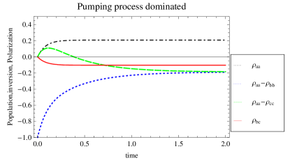
(a) (b)

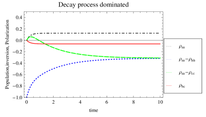
Figure 2: Under initial condition case $I$ :$\rho_{aa}=0,\rho_{bb}=1,\rho_{cc}=0,\rho_{bc}=\rho_{cb}=0$ , upper level population $\rho_{aa}$, population inversion $\rho_{aa}-\rho_{bb}$,$\rho_{aa}-\rho_{cc}$, coherence $\rho_{bc}$.Parameters are $r_{1}=r_{2}=r,\gamma_{1}=\gamma_{2}=\gamma$,Time is measured in units of $\gamma$.(a):no population inversion in the steady state, pumping interaction dominated: $r=2.5\gamma$;(b): no population inversion in the steady state, decaying mechanics dominated: $r=0.5\gamma$

From Fig.2 it’s clear that all levels population do not vary with time in the long run, indicate that the atomic system goes into steady state. For different sets of pumping and decaying parameters, the atomic system goes into different steady states, as show in figure (a)(where pumping rate is set to be greater than the decay rate) and figure (b)(where decay rate is larger than pumping rate). By inspecting all the solutions corresponding to the situations listed in the table.1, we find that the atomic system steps into corresponding steady states for different initial conditions and pumping and decaying parameters sets, thus the system shows a multi-steady state character.

From Fig.2 we find that, the population inversion function $\rho_{aa}-\rho_{bb}$ and $\rho_{aa}-\rho_{cc}$ are both take values below zero, which indicates that there is no population inversion situations appear. And this is the common character of case $I$ after inspecting the other two initial conditions. But for initial conditions in case $II$, population inversion will appear in the steady states. It’s worthy to point out that in one situation of case $II$, initially the two lower level states equally share the total population, and the coherence between them take the ”positive maximum” value $\frac{1}{2}$, the system will evolve into another steady state for nonvanishing pump rate.

The most interesting solutions to the equations (38)-(42) are achieved in case $III$, where initially the two lower states have equal one half of total population and the coherence between them was prepared to the maximal value $-\frac{1}{2}$, it is the ”maximal coherence” generated in the systemPRA063829 . From the results shown in Fig.3 we find out that this is the ”robust” steady state solution in sectionIII.1! It’s clear that for arbitrary sets of pumping $r$ and decay parameters $\gamma$, all three level population $\rho_{aa}$,$-\rho_{bb}$ and $\rho_{cc}$ and the coherence term $\rho_{bc}$ are staying in their initial values, which shows a very stable characteristic.

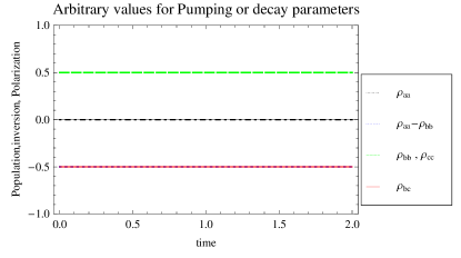
Figure 3: Under initial condition case $III$:$\rho_{aa}=0,\rho_{bb}=\frac{1}{2},\rho_{cc}=\frac{1}{2},\rho_{bc}=\rho_{cb}=-\frac{1}{2}$ , upper level population $\rho_{aa}$, population inversion $\rho_{aa}-\rho_{bb}$ and $\rho_{aa}-\rho_{cc}$,lower level population $\rho_{bb}$ and $\rho_{cc}$, coherence $\rho_{bc}$. The coherence function line is covered by population inversion function lines. Parameters are $r_{1}=r_{2}=r,\gamma_{1}=\gamma_{2}=\gamma$,Time is measured in units of $\gamma$. This is the maximal coherent state situation, where level population does not change as time going by, coherence does not change either.

.

Different from the general steady state solution, these solutions corresponding to situations listed in table.1 are the restrict analytic solutions with variable $t$, which will provide much more system evolution details. Thus by inspecting the way of level population transition and coherence acting in the $\Lambda$ system, we can reveal the mechanism of atomic coherence excitation and preparation the ”robust” steady state, and look for other interesting state as the ”weak” steady state.

From the results of the upper three kinds of situations represented in Fig.2 - Fig.3, we can draw a picture of level population transition. Take the result of Fig.2 for instance, population starts from one of the lower state, the $|b\rangle$ state, while the other two states $|a\rangle$ state and $|c\rangle$ state are empty, and initially the coherence $\rho_{bc}$ is zero, under the interaction of incoherent pump field and vacuum decay process, population transfer to state $|a\rangle$ and state $|c\rangle$. As shown in Fig.2 (a), $|a\rangle$ state population grows up from zero, after a time about $0.5\gamma$, it equals to that of $|c\rangle$ state, and then it does not change with time, indicating that the $|a\rangle$ state has stepped into steady state. The population of the two lower levels are still changing, till time equal to about $1.8\gamma$, state $|c\rangle$ and state $|b\rangle$ are arriving to steady state and their population are equal. As a comparison, in Fig.2 (b), where the pump rate is relatively weak: $r=0.5\gamma$, it costs much long time to reach steady state for states $|b\rangle$ and $|c\rangle$, and this is the same situation for other solutions in different initial conditions.

During the population transition period, the coherent term $\rho_{bc}$ varies from initial value to steady value, for different initial conditions, the coherence term $\rho_{bc}$ takes different values in steady state, from positive values to negative ones, and the varying laws are also different from each other. We would like to inspect the varying law for coherence in a sophisticated way to find out the mechanism of atomic coherence excitation. Depending on different initial conditions shown in table.1, the forms of analytic solutions to coherence $\rho_{bc}$ are different from each other, but for long time limit, they come to an identical one as Eq.(43):

$$\rho_{bc}=\frac{(3r+2\gamma)C_{0}-r}{4(2r+\gamma)}$$ (43)

where $C_{0}$ is the integration constant as defined in Eq.(37), $r$ is the pump rate, $\gamma$ the decay rate. Firstly we fix the value of decay rate $\gamma$ and discuss the law of coherence term varies with pump rate. For initial conditions of $C_{0}=0$, the coherence $\rho_{bc}$ takes negative value, the absolute value of it become larger as pump rate $r$ increases; for initial conditions $C_{0}=1$, the coherence term $\rho_{bc}$ takes positive value, but it will drops with pump rate $r$ increases; for $C_{0}=-1$, coherence $\rho_{bc}=-\frac{1}{2}$, remains unchanged. On the other hand, if we fixed the pump rate $r$ and inspect the varying law for coherence with decay rate, we will get the contrary results. Combining different behaviors of the coherence term $\rho_{bc}$ in Fig.2 - Fig.3, we know that the coherence is induced by the interference of incoherent pumping process and decay process, the two processes contribute different sign to the coherence and interfere destructively. Thus the coherence produces various of steady state results according to different conditions, including the general steady state solution Eq.(19), in which the contribution of decaying process was totally suppressed by incoherent pumping process.

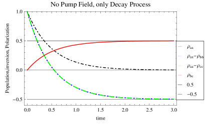
Figure 4: Pumping parameters are set to zero value to inspect the behavior of coherence and steady state characteristic. The coherence $\rho_{bc}$, upper level population $\rho_{aa}$, population inversion $\rho_{aa}-\rho_{bb}$,$\rho_{aa}-\rho_{cc}$ are plotted in different line style. Decay parameters are set to $\gamma_{1}=\gamma_{2}=1.0$ Initial conditions take as case$II$ :$\rho_{aa}=1,\rho_{bb}=0,\rho_{cc}=0,\rho_{bc}=\rho_{cb}=0$, pumping parameters are$r_{1}=r_{2}=0$

.

What will the system state like only by the action of decaying process? It’s suitable to take initial condition of case $II$ to inspect this: $\rho_{aa}=1,\rho_{bb}=0,\rho_{cc}=0,\rho_{bc}=\rho_{cb}=0$, that is, initially the upper state $|a\rangle$ is fully populated, while the two lower states $|b\rangle$ and $|c\rangle$ are empty, the coherence starts from zero value. If we cancel the pump field, the system will then decays, without the disturbances of pumping field, the atomic system will arrive at a positive maximal coherence steady state, in which the upper level has no population, and the two lower levels are equally populated with half of total population:$\rho_{aa}=0,\rho_{bb}=\frac{1}{2},\rho_{cc}=\frac{1}{2}$; and the coherence comes to the positive maximal value, $\rho_{bc}=\frac{1}{2}$, as shown in Fig.4.

Interestingly, the final steady state is equal to the other initial state in case $II$. The density matrix of this steady state take the following form:

$$M=\left[\begin{array}[]{cc}\rho_{bb}&\rho_{bc}\\ \rho_{cb}&\rho_{cc}\end{array}\right]=\left[\begin{array}[]{cc}\frac{1}{2}&\frac{1}{2}\\ \frac{1}{2}&\frac{1}{2}\end{array}\right].$$ (48)

Similarly, if we takes the dual rail representation, the upper state can be expressed as: $|\psi\rangle=\frac{1}{\sqrt{2}}(|01\rangle+|10\rangle)$. But this state is not so stable as the ”robust” state under the driving of nonvanishing pumping field, as discussed in the upper text, we would call it the ”weak” steady state corresponding to the ”robust” steady state. This ”weak” stability indicates the stochastic and incoherent nature of spontaneous decay process, while the ”robust” stability shows the versatile applications of pumping field in level states manipulation and overcoming the stochastic spontaneous. For example, by adjusting the pumping parameters $r_{1}$ and $r_{2}$ according to the decaying rates $\gamma_{1}$ and $\gamma_{2}$, we can generate steady state from the ”robust” steady to the ”weak” steady state, which will be very useful in quantum optics and quantum information science.

IV Discussion and Conclusion

In the above, we have studied the level population transition and the atomic coherence excitation process in the three-level $\Lambda$ atomic system in the joint action of incoherent pumping field and vacuum reservoir, and find out that the system has rich coherence and interference features like that in the action of coherent pumping field, for example, the coherent population trapping (CPT) state can be generated easily. So the upper system under discussion will be very useful in applications to atomic coherence and interference in quantum optics, such as lasing without inversion (LWI), electromagnetically induced transparency (EIT) and quenching spontaneous emission, and so on, which is very similar to that of the $V$ type systemPRA063829 . As a comparison, the CPT state generated in $\Lambda$ system has better quality than that in the $V$ type system, for it’s unrelated to the decay parameters and only relates to the pumping rates. With this better accessibility of the $\Lambda$ system, it will deserve much more recognition in atomic excitation study. But unfortunately, this kind of closely spaced levels structure atomic system is difficult to getPRA063829 , and the experimental implementation of the upper attractive applications seems to be a very difficult job. However the system we are studying still shows interesting features in theoretical research, for example, the two kind of extreme situations for coherence value, i.e.,$\rho_{bc}=\pm\frac{1}{2}$ produce interesting results: the ”robust” steady state and the ”weak” steady state, which will be of great help to inspect the fine mechanism of atomic coherence excitation, and to modify atomic states.

In conclusion, by solving the motion equations of density matrix elements of a closed $\Lambda$ type three-level atomic system under the interaction of incoherent pump field and decay process, we derived a coherent population trapping steady state and multi-steady states with different parameters sets for the atomic system. From the solutions we showed a picture of the level population transferring and revealed the mechanism of atomic coherence excitation: the coherence is produced by the destructive interference of incoherent pumping process and decay process. Owning to different value of coherence, the system is able to generate interesting states as the ”robust” steady states and the ”weak” steady state, which promises fruitful potential applications in quantum optics and in quantum information science.

- [1] K. Zaheer and M. S. Zubairy. Phys. Rev. A, 39:2000–2004, 1989.
- [2] S. E. Harris, J. E. Field, and A. Imamoğlu. Phys. Rev. Lett., 64:1107–1110, 1990.
- [3] S. E. Harris. Phys. Rev. Lett., 62:1033–1036, 1989.
- [4] A. Imamoğlu. Phys. Rev. A, 40:2835–2838, 1989.
- [5] Marlan O. Scully and M. Suhail Zubairy. Quantum Optics. Cambridge University Press, Cambridge, U.K., 1997.
- [6] D.F.Walls and G.J.Milburn. Quantum Optics. Springer-Verlag, Berlin Heidelberg, 1994.
- [7] Shi-Yao Zhu, Ricky C. F. Chan, and Chin Pang Lee. Phys. Rev. A, 52:710–716, 1995.
- [8] Hwang Lee, Pavel Polynkin, Marlan O. Scully, and Shi-Yao Zhu. Phys. Rev. A, 55:4454–4465, 1997.
- [9] Kishore T. Kapale, Marlan O. Scully, Shi-Yao Zhu, and M. Suhail Zubairy. Phys. Rev. A, 67:023804, 2003.
- [10] Victor V. Kozlov, Yuri Rostovtsev, and Marlan O. Scully. Phys. Rev. A, 74:063829, 2006.
- [11] Michael A. Nielsen and Isaac L.Chuang. Quantum Computation and Quantum Information. Cambridge University Press, Cambridge, U.K., 2000. Page287-288, dual-rail representation.