Evolution in random fitness landscapes: the infinite sites model

Abstract

We consider the evolution of an asexually reproducing population in an uncorrelated random fitness landscape in the limit of infinite genome size, which implies that each mutation generates a new fitness value drawn from a probability distribution $g(w)$. This is the finite population version of Kingman’s house of cards model [J.F.C. Kingman, J. Appl. Probab. 15, 1 (1978)]. In contrast to Kingman’s work, the focus here is on unbounded distributions $g(w)$ which lead to an indefinite growth of the population fitness. The model is solved analytically in the limit of infinite population size $N\to\infty$ and simulated numerically for finite $N$. When the genome-wide mutation probability $U$ is small, the long time behavior of the model reduces to a point process of fixation events, which is referred to as a diluted record process (DRP). The DRP is similar to the standard record process except that a new record candidate (a number that exceeds all previous entries in the sequence) is accepted only with a certain probability that depends on the values of the current record and the candidate. We develop a systematic analytic approximation scheme for the DRP. At finite $U$ the fitness frequency distribution of the population decomposes into a stationary part due to mutations and a traveling wave component due to selection, which is shown to imply a reduction of the mean fitness by a factor of $1-U$ compared to the $U\to 0$ limit.

1 Introduction

A fruitful exchange of concepts and methods has taken place between evolutionary population biology and the statistical physics of disordered systems over the past several decades [1, 2, 3]. On the most basic level, one imagines that a biological population evolves by searching a high-dimensional landscape for fitness peaks, in much the same way as a disordered system relaxes towards its low energy configurations [4, 5]. Not surprisingly, extremal statistics arguments play a prominent role in both contexts [5, 6, 7, 8, 9, 10, 11]. To make the analogy more precise, we note that the inheritable characters of an individual (its genotype) are encoded in a genetic sequence (consisting of nucleotide letters or the alleles of genes), which for many purposes can be reduced to a binary sequence $\sigma=(\sigma_{1},...,\sigma_{L})$ of fixed length $L$. For a statistical physicist it is very natural to assign the values $\sigma_{i}=\pm 1$ to the letters, and to treat the sequence as, e.g., a row of spins in the two-dimensional Ising model [12] or a configuration of a quantum spin chain [13]. A fitness landscape is then a real-valued function $W(\sigma)$ on the $L$-dimensional sequence space, analogous to the (negative) energy of the spin system.

The notion of a fitness landscape is a venerable and persistent image in evolutionary biology [14, 15], but it has always been plagued by a certain elusiveness, in the sense that very little is known about the fitness landscapes in which real organisms evolve. This situation may eventually change, as the experimental mapping of genotypic fitness becomes feasible for simple microbial systems [16, 17]. Meanwhile it is reasonable to handle our ignorance of real fitness landscapes by treating $W(\sigma)$ as a realization of a suitably chosen ensemble of random functions. This approach was pioneered by Kauffman and coworkers [7, 8], who introduced the NK family of random fitness landscapes which are closely analogous to Derrida’s $p$-spin model of spin glasses developed a few years earlier [6, 18]. Two limiting cases of the model are of interest here: The random energy model (REM), in which fitness (or energy) is assigned randomly without correlations to the genotypes (or spin configurations), and the case in which the letters $\sigma_{i}$ contribute independently (multiplicatively for discrete time dynamics [15]) to the fitness. In the latter case there is always a single fitness maximum, which explains why this is also referred to as the Fujiyama landscape. In the evolutionary context deviations from multiplicative fitness are associated with epistasis [16]. Within the NK family, the REM landscape is maximally epistatic [19].

In previous work the evolutionary process in the REM landscape has been studied mostly in the limit of infinite population size, where fluctuations due to sampling noise (also known as genetic drift in population genetics) are ignored [15]. While this allows one to derive a rather complete picture of both stationary [20, 21] and time-dependent [22, 23, 24, 25] properties of the model, the assumption of an infinite population is unrealistic, because the number of possible genotypes $2^{L}$ exceeds any conceivable population size $N$ already for moderate values of $L$. On the other hand, individual-based simulation studies which explicitly follow the population through sequence space are restricted to rather short sequences [26, 27].

In this contribution we therefore propose to perform the limit of infinite sequence length at finite population size $N$. This kind of limit is well known in population genetics, where it is viewed alternatively as a limit on the number of genetic loci or sites (the sequence length $L$ in our setting) or as a limit on the number of alleles (the number of possible values that the variables $\sigma_{i}$ can take). Although mathematically distinct, the two variants are equivalent for our purposes.

The implementation of the infinite sites limit for the REM landscape is straightforward: For $L\to\infty$ every mutation leads to a new genotype, whose fitness can be randomly generated without need to keep track of the neighborhood relations of the sequence space. In this way large populations can be simulated efficiently for many generations. Moreover, we show that for long times and small mutation rates the model reduces to a simple point process which is partly tractable analytically. We also present an analytic solution of the infinite population limit of the model, which is useful for describing the evolution of finite populations at early times and provides important insights into the structure of the fitness distribution.

The infinite population version of our model was introduced by Kingman in 1978 [28] and is known as the house of cards model [29]. This term refers to the idea that the genetic organization of an organism is very fragile, such that it is completely disrupted by any change in the genome which therefore leads to a new fitness that is uncorrelated with the fitness of the parent genotype. Previous studies of the finite population dynamics of this model have been concerned mostly with the regime of weak selection, where a balance is established between deleterious and beneficial mutations [30, 31, 32]. In contrast, in the present paper we consider the strong selection regime where the population fitness increases without bound (see section 4.1 for a definition of these regimes).

We give a brief outline of the paper. In the next section we introduce the basic Wright-Fisher dynamics for asexually reproducing populations of constant size $N$, and describe how to implement the infinite sites limit. The evolution of the fitness distribution in the deterministic limit $N\to\infty$ is discussed in section 3. In section 4 we turn to the long-time behavior of finite populations. The key observation is that (for unbounded fitness distributions) fixation events in which a favorable mutation spreads in the population become rare and well-separated as the mean fitness increases. The evolution then reduces to a simple point process closely related to the dynamics of records [9, 11, 33, 34]. We show that to leading order the mean population fitness achieved up to time $t$ is given by the mutation of largest fitness that has been encountered, and we develop an analytic framework to compute sub-leading contributions to the mean fitness and the fitness variance. Finally, conclusions and some open problems are presented in section 5.

2 Wright-Fisher dynamics in the infinite sites limit

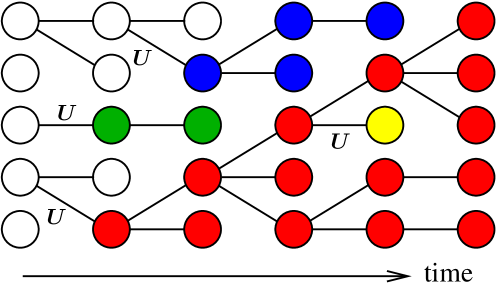
Figure 1: Schematic of the WF model explained in the text. The population size is fixed at $N=5$. Time direction is indicated by the arrow (5 generations). Circles signify the individuals and different colors mean different genotypes which arise by mutation with probability $U$. The vertical location of individuals has no significance (the population is assumed to be well-mixed, without spatial structure). Initially, all individuals have the same genotype (hence the same color). Line segments connecting individuals show who begets whom. Each individual can have only one parent but a parent can have many offspring. After five generations, the red mutation which arose in a single individual at time 2 is fixed in the population (see section 4.1 for further discussion of the fixation process).

We consider a population of $N$ individuals reproducing asexually, in discrete, non-overlapping generations. The basic Wright-Fisher (WF) dynamics [35, 36] of evolution can be described as follows. Each individual $i$ is assigned fitness $w_{i,t}$ ($i=1,\ldots,N$) at generation $t$. Initially, all individuals have the same genotype and accordingly the same fitness $w_{i,0}=1$. At every generation, all individuals are replaced. The probability that a new individual is an offspring of the parent $i$ is proportional to parent’s fitness $w_{i,t}$. To be more accurate, this probability is $w_{i,t}/(\bar{w}_{t}N)$, where $\bar{w}_{t}=\sum_{i=1}^{N}w_{i,t}/N$ is the mean fitness at generation $t$. In the actual simulation, we do not discern different progenitors if they have the same genotype. Instead, the number of progeny of a given genotype is determined from the multinomial distribution with a probability also proportional to the population of that genotype. The multinomial distributed numbers are chosen by sampling correlated binomial random numbers; see, e.g., [37, 38]. Since this reproduction scheme is invariant under the multiplication of a constant to the fitness of all individuals, setting the average initial fitness to unity implies no loss of generality. Once all individuals are replaced, a mutation can change the genotype of each one with probability $U$. A cartoon illustrating the WF model is depicted in figure 1.

In the infinite sites limit, every genotype occurring by mutations can appear only once (there are no recurrent mutations [39]). In the REM landscape the fitness of the mutant is a random number $w$ drawn from some fixed distribution $g(w)$, independent of the number of sites affected by the mutation as well as of the parental genotype. By contrast, the multiplicative fitness landscape is represented in the infinite sites limit by drawing a random selection coefficient $s$ and generating the new fitness $w^{\prime}$ from the parental fitness $w$ by multiplication, $w^{\prime}=(1+s)w$ [37, 40, 41, 42].

The model is completely specified by the population size $N$, the mutation probability $U$ and the choice of the mutation distribution $g(w)$. To make contact with the evolutionary dynamics in a finite space of sequences of length $L$ [27], we note that $U$ is the probability that at least one mutation occurs in a genotype. We therefore have the relation

$$U=1-(1-\mu)^{L}\simeq 1-\exp(-\mu L),$$ (1)

where $\mu$ is the mutation probability per site, and the limit $\mu\to 0$, $L\to\infty$ is implied. Typical values for $U$ range from 0.0025 for E. coli to 0.15 for humans and 0.9985 for the bacteriophage $Q\beta$ [15].

An important difference between the models with finite and infinite genome size is that in the latter case there are no local fitness maxima in which populations can get trapped when $U$ is small [7, 8, 19, 27]. Hence we expect an indefinite increase of the population mean fitness $\bar{w}_{t}$ when the fitness distribution $g$ is unbounded. In the following sections we explore how the behavior of $\bar{w}_{t}$ depends on the model parameters and the choice of $g$. Some representative results from simulations with different values of $N$ and $U$ and the exponential mutation distribution

$$g(w)=e^{-w}$$ (2)

are shown in figure 2. The majority of our results were obtained with the choice (2).

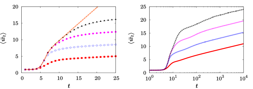
Figure 2: Mean fitness of the WF model for finite and infinite populations. For finite populations, the mean fitness is also averaged over independent runs. The mutation probability $U$ is set to 0.01 and the mutation distribution is $g(w)=e^{-w}$. From bottom to top, the population size $N$ increases ($N=10^{3}$, $10^{5}$, $10^{7}$, and $10^{9}$). The number of independent runs is $8\times 10^{6}\;(N=10^{3})$, $8\times 10^{5}\;(N=10^{5})$, $20~{}000\;(N=10^{7})$, and $4000\;(N=10^{9})$. Left panel shows the short time simulation results and compares them to the infinite population calculation in section 3. Right panel depicts log-linear plots of the mean fitness for finite populations which clearly shows a logarithmic increase of the mean fitness at long times.

3 Infinite populations

In this section, we consider the infinite population dynamics in the REM fitness landscape with an infinite number of sites. In this paper, we take the infinite site $L\to\infty$ limit first, followed by the infinite population limit $N\to\infty$; note that these two limiting procedures do not obviously commute.

3.1 Calculation of the mean fitness

Let $f_{t}(w)dw$ be the fraction of individuals in the population with a fitness between $w$ and $w+dw$. In the limit of infinite population size this evolves deterministically according to [28]

$$f_{t+1}(w)=(1-U)\frac{wf_{t}(w)}{\bar{w}_{t}}+Ug(w),$$ (3)

where $\bar{w}_{t}=\int_{0}^{\infty}dw\;wf_{t}(w)$ is the mean fitness. If $U=1$, trivially and intuitively $f_{t}(w)\equiv g(w)$. The nonlinearity can be removed by introducing [15, 28] $h_{t}(w)=f_{t}(w)\prod_{k=0}^{t-1}\bar{w}_{k}$ with $h_{0}(w)=f_{0}(w)$ which satisfies

$$h_{t+1}(w)=(1-U)wh_{t}(w)+Ug(w)X_{t+1},$$ (4)

where

$$X_{t+1}=\prod_{k=0}^{t}\bar{w}_{k}=\int_{0}^{\infty}dw\;h_{t+1}(w).$$ (5)

The last equality is due to the fact that $f_{t}(w)$ remains normalized. Formally, we can solve the above equation such that

$$\frac{h_{t}(w)}{(1-U)^{t}}=f_{0}(w)w^{t}+Ug(w)\sum_{k=1}^{t}\frac{w^{t-k}X_{k}}{(1-U)^{k}}.$$ (6)

From the self-consistency condition (5), one can find a recursion relation for $X_{t}$,

$$Y_{t}=\phi_{t}+U\sum_{k=1}^{t}Y_{k}G_{t-k},$$ (7)

where $Y_{t}=X_{t}/(1-U)^{t}$, and the quantities

$$\phi_{t}=\int_{0}^{\infty}dw\;f_{0}(w)w^{t},\;\;\;\;G_{t}=\int_{0}^{\infty}dw\;g(w)w^{t}$$ (8)

are moments of the initial condition $f_{0}(w)$ and the fitness distribution $g(w)$, respectively. The recursion relation for $Y_{t}$ can be rewritten in the form

$$Y_{t}=\frac{\phi_{t}}{1-U}+\frac{U}{1-U}\sum_{k=1}^{t-1}Y_{k}G_{t-k},$$ (9)

which is (at least numerically) solvable by iteration. Once we have calculated $Y_{t}$, the mean fitness follows naturally from

$$\bar{w}_{t}=(1-U)\frac{Y_{t+1}}{Y_{t}}.$$ (10)

Although we cannot find a complete analytic expression for $\bar{w}_{t}$, the leading asymptotic behavior can be easily found for some cases. If, for large $t$,

$$G_{t-1}\gg\phi_{t}\;\;\textrm{and}\;\;G_{t}\gg G_{k}G_{t-k}\;\;\textrm{for}\;\textrm{all}\;\;1\leq k\leq t-1,$$ (11)

one can say with small error that

$$Y_{t}\simeq\frac{U}{1-U}Y_{1}G_{t-1}\;\;\Rightarrow\;\;\bar{w}_{t}\simeq(1-U)\frac{G_{t}}{G_{t-1}}.$$ (12)

The criterion (11) is actually not very restrictive. If $g(w)$ has the form of a stretched exponential multiplied by a power law,

$$g(w)=\frac{\beta}{w_{0}\Gamma\left(\frac{\nu+1}{\beta}\right)}\left(\frac{w}{w_{0}}\right)^{\nu}\exp\left(-\left(\frac{w}{w_{0}}\right)^{\beta}\right),$$ (13)

where $w_{0}$ is a constant and $\Gamma(x)$ is the gamma function, the $t$-th moment of $g(w)$ becomes

$$G_{t}=w_{0}^{t}\Gamma\left(\frac{\nu+t+1}{\beta}\right)\Gamma\left(\frac{\nu+1}{\beta}\right)^{-1},$$ (14)

which satisfies (11). Using Stirling’s formula $\Gamma(z)\sim z^{z}e^{-z}\sqrt{2\pi/z}$, one finds that

$$\frac{\bar{w}_{t}}{w_{0}(1-U)}\approx\left(\frac{\nu+t+1}{\beta}\right)^{1/\beta}\sim\left(\frac{t}{\beta}\right)^{\frac{1}{\beta}},$$ (15)

a result that was also reported by Kingman [28].

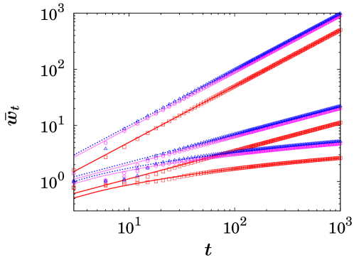
Figure 3: Log-log plots of mean fitness in the infinite population limit as a function of generation $t$ for exponential [$\nu=0$ and $\beta=1$ in (13); upper three data sets], Gaussian [$\nu=0$ and $\beta=2$ in (13); middle three data sets] and Gumbel-type distributions (16) (lower three data sets). For all data sets, $w_{0}$ and $f_{0}(w)$ are set to 1 and $\delta(w-1)$, respectively. For each case, the mutation probability is $U=0.5$ (red), $U=0.1$ (purple), and $U=0.01$ (blue) from bottom to top. The lines are the approximate solutions (15) and (83) with the respective parameters.

When $\beta\rightarrow\infty$, one might expect that the power law (15) turns into a logarithmic increase of the fitness. As an example of an unbounded distribution that decays more rapidly than (13), we consider in Appendix A the Gumbel-type mutation distribution

$$g(w)=\frac{e}{w_{0}}\exp\left(\frac{w}{w_{0}}-e^{w/w_{0}}\right).$$ (16)

Figure 3 compares the exact behavior obtained by iterating (9) to the asymptotic expression (15) and (83) for the exponential, Gaussian, and Gumbel-type distributions. In this comparison, the initial fitness distribution is set to $f_{0}(w)=\delta(w-1)$ and $w_{0}=1$. The analytic approximations are seen to be very accurate in all cases, with error less than 1 % after 100 generations.

Up to now, we have assumed that $G_{t}$ is finite for any $t$. If $g(w)$ has a power law tail

$$g(w)=\alpha(1+w)^{-(\alpha+1)},$$ (17)

however, $G_{t}$ becomes infinite at $t=t_{0}=\{\alpha\}$ where $\{x\}$ means the smallest integer not smaller than $x$. This means that $Y_{t_{0}}$ is finite but $Y_{t_{0}+1}$ is infinite, i.e. $\bar{w}_{t}$ becomes infinite at $t=t_{0}$. This peculiarity of the deterministic selection dynamics has also been observed in the multiplicative case [37], and it is consistent with the behavior of the infinite population dynamics in a finite sequence space, where the population reaches the global fitness maximum in a single time step for large $L$ [23].

For mutation distributions $g(w)$ with bounded support the recursion (3) approaches a limiting distribution $f_{\infty}(w)$ which has been described in detail by Kingman [28]. Remarkably, for certain choices of $g(w)$ one finds a condensation phenomenon in which $f_{\infty}(w)$ develops a $\delta$-function singularity at the maximally possible fitness $w_{\mathrm{max}}$ (set by the upper limit of the support of $g$ or of $f_{0}$, whichever is larger). The asymptotic mean fitness is bounded from below by $(1-U)w_{\mathrm{max}}$. In the remainder of the paper we will restrict the discussion to unbounded mutation distributions.

3.2 Fitness distribution

Note that the mutation rate (provided it is nonzero) enters (15) only through the prefactor $1-U$, which is known in population genetics as the mutational load [29]. Its origin can be traced back to the fact that, in each generation, the fitness is reset randomly for a fraction $U$ of the population, so that selection can act only on the remaining fraction $1-U$ [compare to (3)].

To clarify this effect in a quantitative manner, let us find out what the frequency distribution looks like in the asymptotic regime. To this end, we calculate higher moments of $f_{t}(w)$ from (3) along with (12). For convenience, let

$$\zeta_{n}(t)\equiv\frac{1}{(1-U)w_{0}^{n}}\int w^{n}f_{t}(w)dw.$$ (18)

A recursion relation for the moments can be found by multiplying $w^{n-1}$ to both sides of (3) and integrating over $w$, which yields

$$\zeta_{n}(t)=\zeta_{1}(t)\left(\zeta_{n-1}(t+1)-\frac{U}{1-U}\frac{G_{n-1}}{w_{0}^{n-1}}\right),$$ (19)

and $\zeta_{1}(t)$ can be read off from (12) or (15). The formal solution for $\zeta_{n}(t)$ is

$$\zeta_{n}(t)=\prod_{k=0}^{n-1}\zeta_{1}(t+k)-\frac{U}{1-U}\sum_{k=1}^{n-1}\frac{G_{k}}{w_{0}^{k}}\prod_{\ell=0}^{n-k-1}\zeta_{1}(t+\ell).$$ (20)

Since $w_{0}\zeta_{1}(t)\approx G_{t}/G_{t-1}$ for large $t$, $\zeta_{n}(t)$ becomes

$$(1-U)w_{0}^{n}\zeta_{n}(t)\approx UG_{n}+(1-U)\frac{G_{t+n-1}}{G_{t-1}}-U\sum_{k=1}^{n}\frac{G_{k}G_{t+n-1-k}}{G_{t-1}}.$$ (21)

Constructing the Laplace transform (or the moment generating function) of the frequency distribution using (21) such that

$$\int e^{-zw}f_{t}(w)dw\approx U\tilde{g}(z)+(1-U)\tilde{\varphi}_{t}(z)-U\tilde{\psi}_{t}(z),$$ (22)

where

$$\tilde{g}(z)=\sum_{n=0}^{\infty}\frac{(-z)^{n}}{n!}G_{n}=\int dwe^{-zw}g(w)$$ (23)

is the Laplace transform of $g(w)$ and

$$\tilde{\varphi}_{t}(z)=\sum_{n=0}^{\infty}\frac{(-z)^{n}}{n!}\frac{G_{t+n-1}}{G_{t-1}},\quad\tilde{\psi}_{t}(z)=\sum_{n=1}^{\infty}\frac{(-z)^{n}}{n!}\sum_{k=1}^{n}\frac{G_{k}G_{t+n-1-k}}{G_{t-1}},$$ (24)

we can in turn find the frequency distribution through inverse Laplace transformation. Since the Laplace transformation is linear, $f_{t}(w)$ can be written as

$$f_{t}(w)\approx Ug(w)+(1-U)T_{t}(w)-U\Psi_{t}(w),$$ (25)

where $T_{t}(w)$ and $\Psi_{t}(w)$ are the inverse Laplace transformations of $\tilde{\varphi}_{t}(z)$ and $\tilde{\psi}_{t}(z)$, respectively. Since ($n>1$)

$$G_{n}\ll\sum_{k=1}^{n}\frac{G_{k}G_{t+n-1-k}}{G_{t-1}}\ll\frac{G_{t+n-1}}{G_{t-1}}$$ (26)

because of the criterion (11), we expect that when $w$ is small [large], the dominant contribution for $f_{t}(w)$ comes from $g(w)$ [$T_{t}(w)$]. Hence we neglect the contribution from $\Psi_{t}(w)$, which gives

$$f_{t}(w)\approx Ug(w)+(1-U)T_{t}(w).$$ (27)

For the exponential distribution ($\nu=0,~{}\beta=1$), the analytic form of $\tilde{\varphi}(z)$ can be found. For this case, $G_{t}=w_{0}^{t}t!$, $\tilde{g}(z)=(1+zw_{0})^{-1}$, and

$$\tilde{\varphi}_{t}(z)=\sum_{n=0}^{\infty}\frac{(-z)^{n}}{n!}\frac{G_{t+n-1}}{G_{t-1}}=\sum_{n=0}^{\infty}{t+n-1\choose n}(-zw_{0})^{n}=(1+zw_{0})^{-t}.$$ (28)

Hence the frequency distribution is

$$f_{t}(w)\approx\frac{U}{w_{0}}e^{-\frac{w}{w_{0}}}+\frac{1-U}{w_{0}(t-1)!}\left(\frac{w}{w_{0}}\right)^{t-1}e^{-\frac{w}{w_{0}}}.$$ (29)

One can easily check that the mean and the variance at large $t$ become

$$\bar{w}_{t}\approx(1-U)w_{0}t,\quad\delta w^{2}\approx U(1-U)w_{0}^{2}t^{2},$$ (30)

where $\delta w_{t}^{2}=\int w^{2}f_{t}(w)dw-\bar{w}_{t}^{2}$. Standard deviation and mean are of the same order and $\delta w$ is even larger than $\bar{w}_{t}$ if $U>\frac{1}{2}$. The origin of such a large spread is the division of (29) into two widely separated distributions: A time-independent part, arising from the mutations, and a traveling wave reflecting the selection dynamics. Then the mean and the variance of $T_{t}(w)$ in the asymptotic regime are found to be $tw_{0}$ and $tw_{0}^{2}$, respectively. Hence the spread of $T_{t}$ is much smaller than the mean in the asymptotic regimes, which cannot be appreciated from the full variance in (30). By the central limit theorem, $T_{t}(w)$ is approximated by the Gaussian distribution

$$T_{t}(w)\approx\frac{1}{\sqrt{2\pi tw_{0}^{2}}}\exp\left(-\frac{(w-w_{0}t)^{2}}{2tw_{0}^{2}}\right).$$ (31)

Although we cannot find an analytic form of $f_{t}(w)$ for the general class of distributions (13), the qualitative form is expected to be the same as in the exponential case, that is, a superposition of a stationary distribution due to mutations and a Gaussian travelling wave. Based on this conjecture, we can approximate the travelling wave for the general case. From the generating function of $T_{t}(w)$ which is $\tilde{\varphi}(z)$, one can get the leading behavior of the mean and variance of $T_{t}(w)$ such as

$$-\tilde{\varphi}^{\prime}(0)=\frac{G_{t}}{G_{t-1}}\approx\left(\frac{t}{\beta}\right)^{\frac{1}{\beta}},$$ (32)

$$\tilde{\varphi}^{\prime\prime}(0)-\tilde{\varphi}^{\prime}(0)^{2}=\frac{G_{t+1}}{G_{t-1}}-\left(\frac{G_{t}}{G_{t-1}}\right)^{2}\approx\frac{1}{\beta^{2}}\left(\frac{t}{\beta}\right)^{\frac{2-\beta}{\beta}},$$ (33)

that is, the travelling wave is Gaussian with mean $\bar{w}_{t}/(1-U)$ and width $\sim t^{(2-\beta)/(2\beta)}$.

Since we know the exact values of $\bar{w}_{t}$ from the numerical iteration of (9), we can also numerically calculate the frequency density from (3). Figure 4 numerically confirms for the exponential and Gaussian mutation distribution that the frequency distribution is divided by two parts and the travelling part takes the Gaussian form with the predicted mean and variance in this section. The decomposition (27) will play a considerable role in understanding the behavior of finite populations with large $U$, see section 4.6.

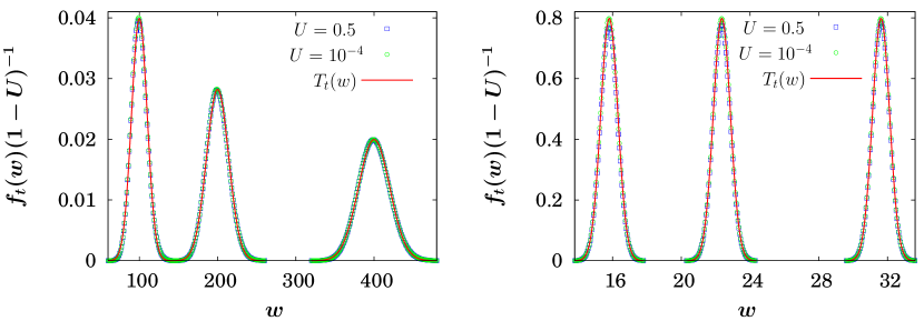
Figure 4: Comparison of the exact numerical solution for the frequency distribution with the travelling wave equation. Left Panel: Frequency distributions at generation $100$, $200$, and $400$ (from left to right) are shown for $U=0.5$ (square) and $U=10^{-4}$ (circle). There is a slight mismatch due to the neglect of $\Psi_{t}(w)$ but ingeneral the travelling wave solution approximate the true distribution quite well. Right panel : Similar study to the Left panel with the Gaussian distribution. The data are collected at generation $500$, $1000$, and $2000$. The Gaussian approximation is almost perfect. The frequency distribution for small $w$ is $Ug(w)$ for both panels as reasoned in the text (data not shown).

4 Finite populations

4.1 Fixation and clonal interference

An important element in the evolution of finite populations is the process of fixation, in which a mutation that is initially present in a single individual spreads in the population and eventually is shared by all individuals (see figure 1 for illustration). Consider the simple case of a single mutant of fitness $w^{\prime}$ entering a genetically homogeneous population in which all individuals have the same fitness $w$. The success of the mutant is determined by the selection coefficient

$$s=\frac{w^{\prime}}{w}-1,$$ (34)

which is positive (negative) for beneficial (deleterious) mutations. For the WF model the fixation probability is given approximately by [44]

$$\pi_{N}(s)\approx\frac{1-e^{-2s}}{1-e^{-2Ns}}.$$ (35)

When selection is strong, in the sense that

$$N|s|\gg 1,$$ (36)

it can be seen from (35) that fixation of deleterious mutations becomes exponentially unlikely, while a beneficial mutation is fixed with probability

$$\pi(s)\approx 1-e^{-2s}.$$ (37)

Previous work on the house of cards model in finite populations has been concerned with the weak selection regime, where $N|s|\approx 1$ [30, 31, 32]. This regime can be realized by choosing a mutation distribution $g(w)$ whose standard deviation is much smaller than the mean. However, in the context of the present paper the strong selection criterion (36) is always satisfied.

The mean time to fixation of a beneficial mutation is given by [44]

$$t_{\mathrm{fix}}\approx\frac{\ln N}{s}.$$ (38)

Different evolutionary regimes arise from the comparison of $t_{\mathrm{fix}}$ to the expected time interval between the emergence of beneficial mutations that are destined for fixation. Denoting by $U_{b}$ the beneficial mutation probability per individual, beneficial mutations arise at rate $NU_{b}$. A mutation fixes with probability $\pi(s_{b})\approx 2s_{b}$, where $s_{b}$ is the typical selection coefficient which is assumed to be small, so that (37) can be approximated by $2s$. Then the waiting time between fixation events is $t_{\mathrm{mut}}\approx 1/(2NU_{b}s_{b})$. When $t_{\mathrm{fix}}\ll t_{\mathrm{mut}}$ or [42]

$$2N\ln NU_{b}\ll 1,$$ (39)

beneficial mutations arise rarely and fix independently, a regime that is referred to as periodic selection [45]. In the opposite case $2N\ln NU_{b}\gg 1$ clones originating from different mutants compete for fixation, a phenomenon that is known as clonal interference [40].

In previous studies of clonal interference [37, 40, 41, 42, 45] it has usually been assumed that $U_{b}$ is a constant parameter, in which case (39) is a condition on the population size $N$ which is violated when $N$ becomes large. However, in a rugged landscape the supply of beneficial mutations decreases as the mean fitness grows. If the fitness distribution of the population is well clustered around its mean $\bar{w}$, the probability of beneficial mutations can be estimated by

$$U_{b}(\bar{w})=U\;\mathrm{Prob}[w>\bar{w}]=U\int_{\bar{w}}^{\infty}dw\;g(w),$$ (40)

which vanishes for $\bar{w}\to\infty$ for any unbounded distribution $g(w)$. Thus clonal interference is a transient phenomenon in rugged fitness landscapes. Asymptotically almost all mutations are deleterious, and hence $U$ can be identified with the probability of deleterious mutations.

4.2 Instantaneous fixation and the diluted record process

The fact that the criterion (39) is asymptotically satisfied for unbounded $g(w)$ implies that the fixation of beneficial mutations occurs as independent events that can then as well be treated as instantaneous ($t_{\mathrm{fix}}\to 0$). Deleterious mutations do not fix, but they lower the mean population fitness through the mutational load $1-U$ (compare to section 3). For the time being, we will neglect this effect, which amounts to taking $U\to 0$. We will show in section 4.6 how the influence of deleterious mutations can be approximately reinstated.

When the effects of deleterious mutations are ignored, the population fitness between fixation events is equal to the fitness of the last beneficial mutation that was successfully fixed, and the population is genetically homogeneous at all times (except for the instances of fixation). The model reduces to a simple point process that can be informally described as follows [31, 32]:

• Mutations with fitness values drawn randomly and independently from $g(w)$ are generated in discrete time according to a Poisson distribution with mean $NU$.

• The fitness of the mutant is compared to the current population fitness; deleterious mutations are discarded while beneficial mutations are fixed with probability $\pi(s)$ given by (37).

• The fitness of the successfully fixed mutant replaces the current population fitness, which therefore evolves according to a piecewise constant, strictly increasing jump process.

If every beneficial mutation were fixed, such that $\pi(s)=\Theta(s)$, the process described above would be identical to a variant of the well-known problem of record statistics for sequences of independent, identically distributed variables [33, 34], in which a Poisson-distributed number of new variables is created in each discrete time step. When $\pi(s)<1$ some of the record events are lost in a way that is correlated to the corresponding record values. The process defined by the rules (i)-(iii) is referred to in the following as the diluted record process (DRP), and it will be studied extensively in the next three subsections.

For long times, when beneficial mutations become increasingly rare, the discrete unit of time is unimportant and the dependence on the system parameters $N$ and $U$ can be eliminated by using the dimensionless time variable $\tau=UNt$. Asymptotically the DRP is therefore fully specified by the functions $\pi(s)$ and $g(w)$. A comparison between the DRP and the full WF dynamics is shown in figure 5. For large $N$ an initial regime can be identified in which clonal interference reduces the fitness in the WF model compared to the DRP, and for large $U$ the fitness is reduced by the mutational load effect, but for long times and $U\ll 1$ the agreement is seen to be essentially perfect. In this and the following three subsections, we restrict ourselves to $U\ll 1$ and the analysis of the behavior for large $U$ is deferred to section 4.6.

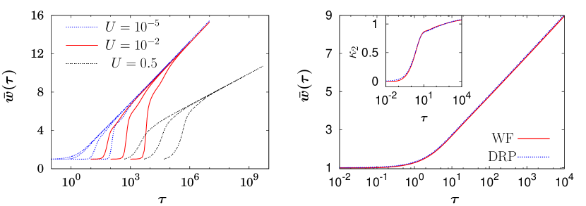
Figure 5: Left panel: Semilogarithmic plots of the fitness vs dimensionless time $\tau=NUt$ for $U=10^{-5}$ ($N=10^{3},\;10^{4},\;10^{5},\;10^{6}$), $U=10^{-2}$ and $U=0.5$ ($N=10^{3},\;10^{4},\;10^{5}$) obtained from simulations of the WF model. The mutation distribution and the initial frequency distribution are same as those in figure 2. Right panel: The comparison of the simulation of the WF model to the DRP for $N=10^{3}$ and $U=10^{-5}$ ($\tau=10^{-2}t$). The difference in the fitness is barely observable. Inset: Same type of the comparison for the variance $\kappa_{2}$ [see (61)] of the fitness.

Clearly the record process (RP) provides an upper bound on the DRP at all times [32]; for completeness, a derivation of the fitness distribution for the RP is provided in Appendix B. We will now argue that the RP bound is in fact saturated for the leading order behavior of the mean fitness, in the sense that

$$\lim_{t\to\infty}\frac{\langle w\rangle_{\mathrm{DRP}}}{\langle w\rangle_{\mathrm{RP}}}=1.$$ (41)

To see why this is so, denote by $w_{1}$ the largest fitness value that has appeared up to time $\tau$, and by $w_{2}$ the largest fitness that has also been fixed. Then $w(\tau)=w_{1}$ in the record process and $w(\tau)=w_{2}$ in the DRP. If $w_{1}$ were asymptotically larger than $w_{2}$ in the sense that $w_{1}/w_{2}\geq C>1$, then the selection coefficient of $w_{1}$ in a background of $w_{2}$ is $s_{12}=w_{1}/w_{2}-1\geq C-1>0$ and the corresponding fixation probability $\pi(s_{12})$ is bounded away from zero. It follows that $w_{1}$ is fixed with finite probability, in contradiction to our assumption that $w_{2}$ is the largest fitness that has been fixed.

We will see later that the average fitness $w_{2}$ at time $\tau$ for the exponential distribution is of order $w_{2}\sim\ln\tau-\ln\ln\tau$, while $w_{1}\sim\ln\tau+\mathrm{const}$. As the difference between the largest and $k$th largest value is of order $\ln k$ for exponential random variables [46], this implies that the rank of $w_{2}$ among the $\tau$ fitness values that have been created up to time $\tau$ is $O(\ln\tau)$.

In the following subsections we will develop some analytic tools to systematically compute the mean fitness and higher fitness moments for the DRP.

4.3 Mean field approximation

In the mean field approximation (MFA) the fitness distribution of the population is characterized only by its mean, which will be denoted by $m(\tau)$ in the following. The probability that a new mutation with arbitrary fitness $w^{\prime}>m$ is fixed is given by

$$p_{\mathrm{fix}}=\int_{m}^{\infty}\pi\left(\frac{w^{\prime}-m}{m}\right)g(w^{\prime})dw^{\prime}=m\int_{0}^{\infty}\pi(x)g(mx+m)dx,$$ (42)

and the waiting time until this happens (in dimensionless units) is $\Delta\tau=1/p_{\mathrm{fix}}$. Once fixation occurs, the population fitness increases by the amount

$$\Delta w=\frac{\int_{m}^{\infty}w^{\prime}\pi\left(\frac{w^{\prime}-m}{m}\right)g(w^{\prime})dw^{\prime}}{\int_{m}^{\infty}\pi\left(\frac{w^{\prime}-m}{m}\right)g(w^{\prime})dw^{\prime}}-m=m\frac{\int_{0}^{\infty}x\pi(x)g(mx+m)dx}{\int_{0}^{\infty}\pi(x)g(mx+m)dx},$$ (43)

and $m(\tau)$ is obtained by solving the differential equation

$$\frac{dm}{d\tau}=\frac{\Delta w}{\Delta\tau}=p_{\mathrm{fix}}\Delta w.$$ (44)

For the exponential distribution (2) this takes the explicit form

$$\frac{dm}{d\tau}=4\frac{m+1}{(m+2)^{2}}e^{-m},$$ (45)

with the solution

$$e^{m}(m+2)+I(m)=4(\tau-\tau_{0})+e^{w_{0}}(w_{0}+2)+I(w_{0}),$$ (46)

where

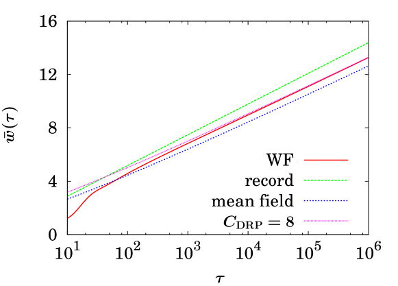
Figure 6: Comparison of the WF simulation with the record, mean field, and the improved approximation scheme in section 4.4 with the stable value of $C_{\mathrm{DRP}}=8$. The WF simulation results are obtained with the exponential mutation distribution (2) with $N=10^{5}$ and $U=10^{-5}$ ($\tau=t$). As explained in the text, mean field theory and record dynamics give lower and upper bounds on the true asymptotics.

$$I(m)\equiv\int_{0}^{m}\frac{e^{x}}{x+1}dx\sim\sum_{n=0}^{\infty}n!\left(\frac{e^{m}}{(m+1)^{n+1}}-1\right).$$ (47)

The asymptotic expansion which is a divergent series is obtained by integration by parts. Now assume that $\tau$ is extremely large, then the approximate inversion formula of (46) will be the solution of the equation

$$me^{m}\approx 4\tau\;\;\;\Rightarrow\;\;\;\;m+\ln m\approx\ln(4\tau).$$ (48)

From (48), one can easily see that $\lim_{\tau\rightarrow\infty}\ln\tau/m=1$. Let $m(\tau)=(1+f(\tau))\ln(4\tau)$ where $f(\tau)\rightarrow 0$ as $\tau\rightarrow\infty$. Then

$$f(\tau)\ln(4\tau)+\ln\ln(4\tau)+\ln(1+f(\tau))=0\;\;\;\rightarrow\;\;\;f(\tau)\approx-\frac{\ln\ln 4\tau}{1+\ln 4\tau},$$ (49)

which, as expected, approaches zero in the asymptotic regime. According to extreme value statistics, the largest fitness up to time $\tau$ is of order $\ln\tau+\gamma$, where $\gamma(\approx 0.5772)$ is the Euler number. But the leading behavior of $m(\tau)$ is $\ln\tau+\ln 4$, which seems contradictory. This apparent paradox can be resolved by looking at the difference $\ln(\tau)-m(\tau)=O(\ln\ln t)>0$, which diverges for $\tau\to\infty$. In figure 6, the MFA solution (48) with the correction (49) is compared to the WF simulation and the record problem.

For fitness distributions with a power law tail (17), we get ($\alpha>1$)

$$p_{\mathrm{fix}}=\alpha m^{-\alpha}J(\alpha+1,m),\quad\Delta w=m\frac{J(\alpha,m)-J(\alpha+1,m)}{J(\alpha+1,m)}-1,$$ (50)

where

$$J(\alpha,m)=\int_{1}^{\infty}\left(1-e^{-2(x-1)}\right)\left(\frac{1}{m}+x\right)^{-\alpha}dx.$$ (51)

To have a meaningful result, we should restrict ourselves to the case $\alpha>1$. Hence (44) for the power law case becomes

$$\eqalign{\frac{dm}{d\tau}&=\alpha m^{-\alpha+1}(J(\alpha,m)-J(\alpha+1,m))-\alpha m^{-\alpha}J(\alpha+1,m)\\ &\approx\alpha m^{-\alpha+1}(K(\alpha)-K(\alpha+1)),}$$ (52)

where $K(\alpha)=J(\alpha,\infty)$. Evaluation of the differential equation (52) in the asymptotic regime ($m\gg 1$) yields

$$m\approx\tau^{1/\alpha}(\alpha^{2}(K(\alpha)-K(\alpha+1))^{1/\alpha}\equiv\tau^{1/\alpha}L(\alpha).$$ (53)

To complete the analysis, let us compare $L(\alpha)$ to the prefactor obtained in (92) for the record process. When $\alpha-1\ll 1$, the two prefactors have the expansion

$$\eqalign{L(\alpha)=\frac{1}{\alpha-1}+\ln(\alpha-1)+0.916~{}014+o(1),\\ \Gamma\left(\frac{\alpha-1}{\alpha}\right)=\frac{1}{\alpha-1}+(1-\gamma)+o(1),}$$ (54)

which shows that the RP prefactor is larger than that of the MFA in this regime. When $\alpha\gg 1$, the asymptotic behavior of the MFA prefactor can be obtained by integration by parts. One finds

$$\eqalign{L(\alpha)=1+\frac{1}{\alpha}\ln(4/\alpha)+o(1/\alpha)<1,\\ \Gamma\left(1-\frac{1}{\alpha}\right)=1+\frac{\gamma}{\alpha}+o(1/\alpha)>1,}$$ (55)

which also suggests that the MFA prediction is smaller than the RP value. Actually, the MFA prefactor becomes smaller than unity when $\alpha>3.533~{}18$ while $\Gamma((\alpha-1)/\alpha)$ remains larger than unity. In between, one can numerically check that the RP prefactor is always larger than that of the MFA. In fact, we will show in the next subsection that the MFA always provides a lower bound on the true mean fitness of the DRP. To summarize the mean field theory for the power law distribution, the MFA fitness is of the same order as the extremal statistics estimate (93), but the smaller prefactor is not consistent with the relation (41).

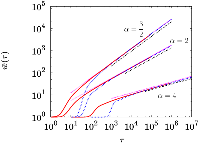
Figure 7: Log-log plots of $\bar{w}(\tau)$ vs $\tau$ for the simulation results of the WF dynamics with the power law distribution (17) with $\alpha=\frac{3}{2}$ (upper data set), $\alpha=2$ (middle data set), and $\alpha=4$ (lower data set). The mutation probability is set to $U=10^{-4}$ and the population sizes are $10^{4}$ and $10^{5}$ for $\alpha=\frac{3}{2}$ and 2, and $10^{5}$ and $10^{6}$ for $\alpha=4$, respectively. For comparison, the record solution (92) (straight line segments above the simulation results) and the MF prediction (53) (straight line segments below the simulation results) are also depicted.

Figure 7 compares the WF simulation results with the record solution (92) and the MF result (53) for three values of $\alpha$. For $\alpha=\frac{3}{2}$, the RP result is in good agreement with the WF simulations but as $\alpha$ increases, both bounds increasingly deviate from the simulation data. Since for $\alpha\rightarrow\infty$ the power law distribution approaches a distribution of exponential type, the results for the exponential distribution summarized in figure 6 indicate that a similar discrepancy should be expected for larger values of $\alpha$. For $\alpha\leq 2$, the variance of the distribution of record values is infinite, which implies that the value of a new record is usually much larger than the previous record and $\pi(s)\approx 1$. In this case the DRP becomes identical to the RP. On the other hand, as $\alpha$ gets bigger, the ratio of two consecutive records approaches unity in the asymptotic regime. This implies stronger corrections to the leading behavior which, according to (41), should still be given by the RP.

4.4 Master equation

To improve on the mean field approximation, we will first derive an equation for the transition probability $p(w,\tau|w_{0},0)$ of the DRP [19, 31]. Since the model is a Markov process, the conditional probability $p(w,t+dt|w^{\prime},t^{\prime})$ completely specifies the evolution equation. We have

$$\eqalign{p(w,\tau+d\tau|w^{\prime},\tau)=&\delta(w-w^{\prime})\left(1-d\tau\int_{w^{\prime}}^{\infty}\pi\left(\frac{x-w^{\prime}}{w^{\prime}}\right)g(x)dx\right)\\ &+d\tau\Theta(w-w^{\prime})g(w)\pi\left(\frac{w-w^{\prime}}{w^{\prime}}\right).}$$ (56)

Using the Markov property, the equation for $p(w,\tau)\equiv p(w,\tau|w_{0},\tau_{0})$ can be found as follows:

$$\eqalign{p(w,\tau+d\tau)=\int dx\;p(w,\tau+d\tau|x,\tau)p(x,\tau)\\ =p(w,\tau)\left(1-d\tau\int_{w}^{\infty}\pi\left(\frac{x-w}{w}\right)g(x)dx\right)+g(w)d\tau\int_{w_{0}}^{w}\pi\left(\frac{w-x}{x}\right)p(x,\tau)dx,}$$ (57)

and therefore

$$\frac{dp(w,\tau)}{d\tau}=-p(w,\tau)\int_{w}^{\infty}\pi\left(\frac{x-w}{w}\right)g(x)dx+g(w)\int_{w_{0}}^{w}\pi\left(\frac{w-x}{x}\right)p(x,\tau)dx.$$ (58)

The description by the master equation (58) is appropriate for a Markov process like the DRP which has non-continuous sample paths [47]. One can easily check that the record probability (86) solves (58) when $\pi(x)=\Theta(x)$.

From (58) evolution equations for arbitrary expectation values $\langle f(w,\tau)\rangle$ can be obtained in the form

$$\eqalign{\frac{d}{d\tau}\langle f(w,\tau)\rangle\equiv\frac{d}{d\tau}\int dw\;p(w,\tau)f(w,\tau)=\int dw\left(f(w,\tau)\frac{\partial p(w,\tau)}{\partial\tau}+\frac{\partial f(w,\tau)}{\partial\tau}p(w,\tau)\right)\\ =\left\langle w\int_{0}^{\infty}\left[f(wx+w,\tau)-f(w,\tau)\right]\pi(x)g(wx+w)dx\right\rangle+\left\langle\frac{\partial f(w,\tau)}{\partial\tau}\right\rangle.}$$ (59)

For example, the equation for the centered normalized moment $\kappa_{n}\equiv(w-\langle w\rangle)^{n}/n!$ is

$$\frac{d\langle w\rangle}{d\tau}=\left\langle w^{2}\int_{0}^{\infty}x\pi(x)g(wx+w)dx\right\rangle,$$ (60)

$$\frac{d\kappa_{n}}{d\tau}=\sum_{r=1}^{n}\left\langle\frac{w^{r+1}}{r!}\frac{(\delta w)^{n-r}}{(n-r)!}\int_{0}^{\infty}dxx^{r}\pi(x)g(wx+w)\right\rangle-\kappa_{n-1}\frac{d\langle w\rangle}{d\tau},$$ (61)

where $\delta w\equiv w-\langle w\rangle$. For the cases of the exponential distribution (2) and the power law (17), (60) becomes

$$\frac{d\langle w\rangle}{d\tau}=\left\langle\frac{4(w+1)}{(w+2)^{2}}e^{-w}\right\rangle,$$ (62)

$$\frac{d\langle w\rangle}{d\tau}=\alpha\left\langle w^{-\alpha+1}(J(\alpha,w)-J(\alpha+1,w))-w^{-\alpha}J(\alpha+1,w)\right\rangle,$$ (63)

which reduce to the mean field equations (45) and (52) if we approximate $\langle\chi(w)\rangle\approx\chi(\langle w\rangle)$, where $\chi(w)$ is the function inside the brackets on the right hand side of (62,63). Again note that (63) is meaningful only if $\alpha>1$. Since $\chi(w)$ is a convex function asymptotically, that is, $\chi^{\prime\prime}(w)>0$ for $w\gg 1$, $\chi(\langle w\rangle)\leq\langle\chi(w)\rangle$, which means that the mean field theory yields a lower bound on the true asymptotics.

4.5 Moment expansion

We now develop a systematic approximation scheme which extends beyond mean field theory. First we write down the differential equations for $m\equiv\langle w\rangle$, $\kappa_{2},\ldots,\kappa_{\ell}$ which are available from Eqs. (60) and (61) once $g(w)$ is given. Then we expand the terms on the right hand side, of the general form $\langle\chi(w)\rangle$, up to $\kappa_{\ell}$ in such a way that

$$\langle\chi(m+\delta w)\rangle=\chi(m)+\kappa_{2}\frac{d^{2}\chi(m)}{dm^{2}}+\kappa_{3}\frac{d^{3}\chi(m)}{dm^{3}}+\ldots$$ (64)

and keep terms only up to $\kappa_{\ell}$ in all equations for $\kappa_{n}$ ($\ell\geq n$). If we only keep terms up to $\ell=1$, then we arrive at the mean field equation. If we keep terms up to $\ell=2$, then we have

$$\eqalign{\frac{dm}{d\tau}&=\frac{4(m+1)}{(m+2)^{2}e^{m}}+\frac{4(m^{3}+7m^{2}+14m+2)}{(2+m)^{4}e^{m}}\kappa_{2},\\ \frac{d\kappa_{2}}{d\tau}&=\frac{2(3m^{2}+6m+4)}{(m+2)^{3}e^{m}}-\frac{2(m^{4}+8m^{3}+30m^{2}+68m+16)}{(m+2)^{5}e^{m}}\kappa_{2}}$$ (65)

for exponential $g(w)$. Since we are interested in the asymptotic behavior, the above equations are approximated for large $m$ by

$$\frac{dm}{d\tau}\simeq\frac{4}{me^{m}}(1+\kappa_{2}),\quad\frac{d\kappa_{2}}{d\tau}\simeq\frac{2}{me^{m}}(3-\kappa_{2}).$$ (66)

Thus we see that $\kappa_{2}\rightarrow 3$ and the mean field equation for $m$ receives a multiplicative fluctuation correction. By increasing $\ell$, the solution should become more accurate.

Clearly the above scheme can not be applicable to all $g(w)$. For example, if $g(w)$ has a power law tail (17), $\kappa_{n}$ is infinite if $n\geq\{\alpha\}$. However, even if $\kappa_{n}$ is well defined for all $n$, it is not at all guaranteed that the solution for $\langle w\rangle$ becomes better as we take more and more $\kappa_{n}$ into account. To clarify this point, let us think about the record problem for the exponential distribution (2) which corresponds to $\pi(x)=\Theta(x)$ and is exactly solvable. For this case (60) and (61) yield

$$\frac{dm}{d\tau} = \langle e^{-w}\rangle=e^{-m}\langle e^{-\delta w}\rangle\sim e^{-m}\sum_{k=0}^{\infty}(-1)^{k}\kappa_{k},$$ (67)

$$\frac{d\kappa_{n}}{d\tau} = \left\langle e^{-w}\left[\left(\sum_{r=0}^{n-1}\frac{(\delta w)^{r}}{r!}\right)-\kappa_{n-1}\right]\right\rangle$$ (68)

$$\sim e^{-m}\left(\sum_{r=0}^{n-1}\sum_{k=0}^{\infty}{k+r\choose k}(-1)^{k}\kappa_{r+k}-\kappa_{n-1}\langle e^{-\delta w}\rangle\right)$$

where $\kappa_{0}=1$ and $\kappa_{1}=0$ by definition and $\sim$ means that the order of summation and integration is interchanged (without any legitimation). The approximation scheme described above implies that we keep terms only up to $\ell$ in (67,68). Now assume that this solution becomes exact as $\ell\rightarrow\infty$. If this is true, we expect that $\kappa_{k}\rightarrow M_{k}/k!$ as $\tau\rightarrow\infty$ where $M_{k}$ is defined in (88). Naively interchanging the order of summation and integration, we then get

$$\langle e^{-\delta w}\rangle\sim\sum_{k=0}^{\infty}(-1)^{k}\frac{M_{k}}{k!}\sim\int_{0}^{\infty}\sum_{k=0}^{\infty}\frac{(\gamma+\ln x)^{k}}{k!}e^{-x}dx=e^{\gamma},$$ (69)

which along with (67) gives the exact asymptotic behavior $m\sim\ln\tau+\gamma$. Similarly we obtain by commuting summation and integration that

$$\sum_{r=0}^{n-1}\sum_{k=0}^{\infty}{k+r\choose k}(-1)^{k}\kappa_{r+k}\sim e^{\gamma}\sum_{r=0}^{n-1}I_{r}=\kappa_{n-1}e^{\gamma},$$ (70)

where

$$I_{r}=\frac{1}{r!}\int_{0}^{\infty}(-\gamma-\ln x)^{r}xe^{-x}dx=\kappa_{r}-\kappa_{r-1}$$ (71)

for $k\geq 1$ and $I_{0}=1$. Thus it seems that our approximation scheme solves the problem accurately as $\ell$ increases.

However, this agreement is in fact fortuitous. Equation (69) illustrates the problem. One can easily see that $\langle e^{-\delta w}\rangle$ is indeed equal to the integral yielding $e^{\gamma}$, but the intermediate series $S_{\ell}\equiv\sum_{k=0}^{\ell}(-1)^{k}\kappa_{k}$ is actually not convergent. In fact, even if we use the exact values for $\kappa_{n}$, $S_{\ell}$ oscillates between 1.500 34 and 2.0618 whose average is 1.781 07 $=e^{\gamma}$. We conclude, therefore, that the approximation scheme can at best be expected to yield an asymptotic series.

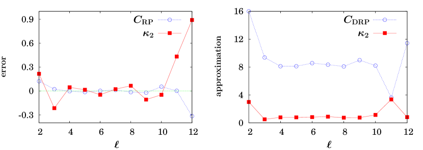
Figure 8: The results of the approximation scheme for the mean ($C_{\mathrm{RP}}$ and $C_{\mathrm{DRP}}$) and variance ($\kappa_{2}$) including terms up to $\kappa_{\ell}$ for the RP (left panel) and for the DRP (right panel). Since we know the exact value of $C_{\mathrm{RP}}$ and $\kappa_{2}$ for the record problem, in the left panel we compare the approximation to the exact values.

Despite this difficulty, we now demonstrate that the moment expansion yields reliable results when used with caution. We have applied the scheme to the record problem and the DRP with exponential $g(w)$. Assuming that all $\kappa_{n}$ will saturate as $\tau\rightarrow\infty$, the mean fitness then follows an equation of the form

$$\frac{dm}{d\tau}\approx C_{\mathrm{RP}}(\ell)e^{-m},$$ (72)

for the record process

$$\frac{dm}{d\tau}\approx\frac{C_{\mathrm{DRP}}(\ell)}{me^{m}},$$ (73)

for the DRP, respectively. The argument $\ell$ means that the constants $C_{\mathrm{RP}}$ and $C_{\mathrm{DRP}}$ are evaluated keeping the $\kappa_{n}$ up to $n=\ell$. For instance, we have already shown that $C_{\mathrm{DRP}}(1)=4$ from (45) and $C_{\mathrm{DRP}}(2)=16$ from (66).

Figure 8 summarizes the results of the approximate evaluation of the $C$’s and of $\kappa_{2}$ with increasing $\ell$. In the range $4\leq\ell\leq 10$, the approximation yields rather stable values. The comparison with the exact results for the record problem shows that the method is excellent in this range. However, for $\ell$ larger than 10, the error becomes uncontrollable. In fact, the solutions for $\ell>10$ in figure 8 are meaningless because some $\kappa_{2n}$’s are negative which should be positive. The approximation suggests that $C_{\mathrm{DRP}}\approx 8$, which gives a highly accurate estimate of the asymptotic fitness, see figure 6. On the other hand, the estimate $\kappa_{2}\approx 0.8$ appears to be somewhat smaller than the simulation results, see the inset of the right panel in figure 5.

4.6 Finite $U$

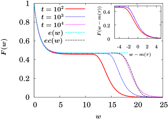
Figure 9: The cumulative frequency distribution for $N=10^{5}$ and $U=0.5$ at $t=10^{2}$, $10^{3}$, and $10^{4}$ (from left to right). The data are collected from $64~{}000$ independent simulations. The approximate expressions $e(w)$ in (76) and $ec(w)$ in (77) with $\xi=0.4725$ are also drawn for comparison. Inset: same but the abscissa is shifted by the amount $m(\tau)$ which is the solution of (73) with $C_{DRP}=8$. The data sets for $t=10^{3}$ and $t=10^{4}$ show a nice collapse.

Until now, the mutation probability $U$ has been assumed to be very small. The natural extension of the previous study is to ask what will happen if the mutation rate is high, which is the topic of this subsection.

One can get some insight from the infinite population calculation in section 3, where it was shown that the frequency distribution can be approximated by a superposition (27) of two distributions which are well-separated from each other. This is still expected to happen in the finite population case when the mean fitness is much larger than the average fitness due to mutations [the average of $g(w)$]. Figure 9 depicts the cumulative frequency distribution obtained from simulations of the WF model at $t=10^{2}$, $10^{3}$, and $10^{4}$ for $N=10^{5}$ and $U=0.5$, defined as

$$F(w)\equiv\left\langle\int_{w}^{\infty}f_{t}(x;N)dx\right\rangle,$$ (74)

where $\langle\ldots\rangle$ means an average over independent samples and $f_{t}(w;N)$ is the frequency distribution for population size $N$. As expected, the cumulative distribution displays a plateau corresponding to the region of low probability between the two peaks, but in contrast to the ansatz (27) the height of the plateau is below $U$. To get a quantitative explanation of this effect, we assume that the frequency distribution is of the form $f_{t}(w;N)=(1-\xi)g(w)+\xi\delta(w-m)$, where $\xi$ is the weight of the high fitness peak which is approximated by a $\delta$-function when $m\gg 1$. Then the population fraction of the genotype with fitness $m$ increases after selection to $\xi m/(\xi m+1-\xi)$, out of which only a fraction $1-U$ remains after mutation. If $m$ and $\xi$ change slowly on the time scale of one generation, one obtains the stationarity condition

$$\xi=\frac{(1-U)\xi m}{\xi m+1-\xi}\rightarrow\xi=(1-U)-\frac{U}{m-1},$$ (75)

which shows that $\xi$ approaches $1-U$ only for $m\to\infty$. This suggests that the cumulative distribution should take the form

$$F(w)\approx e(w)\equiv(1-\xi)g(w)+\xi,$$ (76)

for $w<m$. For the case considered in figure 9, the mean fitness at $t=10^{4}$ is $\approx 19.15$ which gives $\xi\approx 0.4725$ in good agreement with the simulation data. Due to the logarithmic increase of $m$ with $t$ in the case of exponential $g(w)$, the approach to the asymptotic value $\xi\to 1-U$ is very slow. For example, to reach $\xi=0.49$ requires to simulate $t\sim 10^{16}$ generations for our parameters.

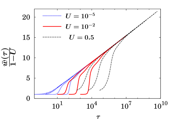
Figure 10: Plots of $\bar{w}(\tau;U)/(1-U)$ vs $\tau$ for the data sets in the left panel of figure 5. All curves now collapse in the asymptotic regime.

For a more accurate description of the high-fitness part of the frequency distribution we assume that, as in the infinite population case, the travelling wave contribution in the decomposition (27) becomes Gaussian at long times. If this is true, the cumulative frequency distribution should take the form

$$F(w)\approx ec(w)\equiv\frac{\xi}{2}\mathrm{erfc}\left(\frac{w-m(\tau)}{2\sqrt{\kappa_{2}}}\right),$$ (77)

where $\mathrm{erfc}$ is the complementary error function and $\kappa_{2}(\approx 0.8)$ is obtained from the analysis of the DRP in the previous section. As shown in figure 9, $ec(w)$ approximates the numerical data quite well, and the distributions obtained at different times $10^{3}$ and $10^{4}$ collapse (inset of figure 9). Though $ec(w)$ is not excellent, we would say that it is a reasonable approximation in the asymptotic regime.

As a consequence of these considerations, the effect of the mutational load on the mean fitness is found to be remarkably simple: Asymptotically we have

$$\bar{w}(\tau;U)\approx\xi m(\tau)+(1-\xi)=(1-U)m(\tau)$$ (78)

where $m(\tau)$ is the mean fitness of the DRP. This prediction is confirmed in figure 10.

5 Conclusions

In this paper we have explored several aspects of the evolution of an asexually reproducing population in a random fitness landscape which (in the sense of the NK family [8, 19]) is maximally epistatic. In contrast to previous work on the REM fitness landscape [20, 21, 23, 26, 27] we adopt the limit of infinite genome length, which leads to a finite population version of Kingman’s house of cards model [28]. Although the model can hardly be expected to provide a realistic description of empirical fitness landscapes [16, 17], it serves as a useful counterpart to the much studied non-epistatic multiplicative landscape model and can help to develop some intuition for the generic features of adaptation under strong epistasis.

An example for such a generic feature is the slowing down of the speed of adaptation compared to the multiplicative model, which reflects the fact that the supply of beneficial mutations dwindles with increasing fitness. This effect is well documented in evolution experiments with microbial populations [48, 49, 50]; in fact, it has been argued [9] that the data obtained by Lenski and Travisano [48] for populations of E. coli can be quantitatively described as a logarithmic increase in fitness, which would be consistent with our finite population results for exponential $g(w)$.

We have extended Kingman’s analysis of the infinite population limit to include the shape of the frequency distribution, which was found to become bimodal at long times. The finite population dynamics was shown to reduce to a diluted record process (DRP) for long times and small mutation probability $U\ll 1$. This representation allows to bound the mean population fitness from above by the standard record process and from below by a mean field approximation to the DRP, which can be improved systematically through a moment expansion. Although connections between record statistics and evolutionary processes have been suggested before [7, 8, 9, 10, 11, 32], we have here for the first time established a precise quantitative relation of the theory of records to one of the cornerstones of population genetics, the WF model. Finally, using insights from the infinite population case, we have shown that the fitness distribution at large $U$ can be understood as a superposition of the DRP distribution and the mutation distribution $g(w)$.

A number of important questions concerning this model are left to future work. For example, it would be interesting to consider the finite population dynamics for bounded mutation distributions $g(w)$, for which the infinite population calculation predicts the appearance of singularities in the stationary fitness distribution [28]. Furthermore, the temporal statistics of the fixation events should be investigated with regard to its relation to record dynamics, for which detailed results are available [33, 34], as well as in comparison to recent work on the corresponding issue for multiplicative fitness landscapes [37].

Appendix A: Infinite population calculation for Gumbel-type $g(w)$

The first step is the calculation of the $t$-th moment of (16),

$$G_{t}=\int w^{t}g(w)dw=ew_{0}^{t}\int_{1}^{\infty}(\ln(y))^{t}e^{-y}dy.$$ (79)

To get an asymptotic expression, let us make a change of variables $y=xt/\ln t$

$$\eqalign{G_{t}&=\frac{etw_{0}^{t}}{\ln t}\left(\ln\left(\frac{t}{\ln t}\right)\right)^{t}\int_{\frac{\ln t}{t}}^{\infty}dx\left(1+\frac{\ln x}{\ln\frac{t}{\ln t}}\right)^{t}\exp\left(-\frac{t}{\ln t}x\right)\\ &=\frac{etw_{0}^{t}}{\ln t}\left(\ln\left(\frac{t}{\ln t}\right)\right)^{t}\int_{\frac{\ln t}{t}}^{\infty}dx\exp\left(-\frac{t}{\ln t}\left\{x-\ln t\ln\left(1+\frac{\ln x}{\ln\frac{t}{\ln t}}\right)\right\}\right).}$$ (80)

Since $t$ is assumed to be very large, the integral is dominated by the regime where the terms in the curly bracket attain a minimum which is easily seen to be unique. One can show that the contribution from the boundaries of the integral is exponentially small and the maximal contribution comes from the region around $x_{c}$ which is the solution of the equation

$$(1-x_{c})\ln t=x_{c}(\ln x_{c}-\ln\ln t)\Rightarrow x_{c}\simeq 1+\frac{\ln\ln t}{\ln t}+O\left(\frac{\ln\ln t}{\ln t}\right)^{2}.$$ (81)

Expanding the terms in the curly bracket around $x_{c}$ and performing the Gaussian integral, we get

$$G_{t}\simeq ew_{0}^{t}\sqrt{\frac{2\pi t}{\ln t}}\left(\ln\left(\frac{t}{\ln t}\right)\right)^{t}\exp\left(-\frac{t}{\ln t}\left\{x_{c}-\ln t\ln\left(1+\frac{\ln x_{c}}{\ln\frac{t}{\ln t}}\right)\right\}\right).$$ (82)

Hence in the long run, the Gumbel-type distribution also meets the criterion (11) and the mean fitness becomes

$$\bar{w}_{t}\approx w_{0}(1-U)\ln\frac{t}{\ln t}\exp\left(\frac{\ln\ln t}{(\ln t)^{2}}\left(1+\frac{\left(\frac{3}{2}\ln\ln t-1\right)}{\ln t}\right)\right),$$ (83)

which increases logarithmically for long times.

Appendix B: Record dynamics

Here we derive an expression for the record probability distribution $p_{\mathrm{RP}}(w,\tau)$ of the population fitness at scaled time $\tau$, in the long time limit where the generation of new random variables is equivalent to a Poisson process in continuous time [51]. During time $\tau$, the probability that there are $n$ mutations is $e^{-\tau}\tau^{n}/n!$. Hence the probability for the fitness at time $\tau$ to be larger than $x$ is

$$\mathrm{Prob}[w>x,\tau]=\sum_{n=0}^{\infty}e^{-\tau}\frac{\tau^{n}}{n!}\left(1-(1-Q(x))^{n}\right)=1-\exp(-\tau Q(x)),$$ (84)

where $Q(x)=\int_{x}^{\infty}dw\;g(w)$ is the cumulative mutation distribution and $x$ is larger than the initial value $w_{0}$ of the process. In addition there is a contribution from the possibility that no new record has appeared up to time $\tau$,

$$\mathrm{Prob}[w=w_{0},\tau]=1-\mathrm{Prob}[w>w_{0},\tau]=\exp(-\tau Q(w_{0})).$$ (85)

Together the two contributions yield

$$p_{\mathrm{RP}}(w,\tau)=\tau g(w)e^{-\tau Q(w)}\Theta(w-w_{0})+e^{-\tau Q(w_{0})}\delta(w-w_{0}),$$ (86)

from which moments and cumulants can be derived. For example, for the exponential case with $g(w)=Q(w)=e^{-w}$ we obtain

$$\langle w\rangle_{\mathrm{RP}}-w_{0}e^{-\tau e^{-w_{0}}}=\int_{w_{0}}^{\infty}dw\;w\tau e^{-w}e^{-\tau e^{-w}}=\ln\tau+\gamma+O(e^{-\tau e^{-w_{0}}}),$$ (87)

$$\langle(w-\langle w\rangle_{\mathrm{RP}})^{n}\rangle_{\mathrm{RP}}=\int_{0}^{\infty}(-\gamma-\ln x)^{n}e^{-x}dx+O(e^{-\tau e^{-w_{0}}})\rightarrow M_{n},$$ (88)

where $\gamma(\approx 0.5772)$ is the Euler number. Hence

$$\langle w\rangle_{\mathrm{RP}}\approx\ln\tau+\gamma,\;\;\;\langle(w-\langle w\rangle_{\mathrm{RP}})^{2}\rangle_{\mathrm{RP}}\approx M_{2}=\frac{\pi^{2}}{6},$$ (89)

which is consistent with extreme value statistics [46]. For a Gaussian $g(w)=2e^{-w^{2}}/\sqrt{\pi}$, one finds

$$\eqalign{\langle w^{n}\rangle_{\mathrm{RP}}&\approx\tau\int_{0}^{\mathrm{erfc}(w_{0})}(\mathrm{erfc}^{-1}(y))^{n}e^{-\tau y}dy\approx\int_{0}^{\infty}\left(\ln(c\tau)-\ln x\right)^{n/2}e^{-x}dx\\ &\approx(\ln(c\tau))^{\frac{n}{2}}+\frac{n}{2}(\ln(c\tau))^{\frac{n}{2}-1}\gamma+\frac{n^{2}-2n}{8}(\ln(c\tau))^{\frac{n}{2}-2}\left(\gamma^{2}+\frac{\pi^{2}}{6}\right),}$$ (90)

where $\mathrm{erfc}$ is the complementary error function $\mathrm{erfc}(x)=\frac{2}{\sqrt{\pi}}\int_{x}^{\infty}e^{-y^{2}}dy$ and $\mathrm{erfc}^{-1}(y)$ is its inverse function whose leading asymptotic behavior is $(\ln c-\ln y)^{1/2}$ with $c=\sqrt{2/\pi}$ when $y\ll 1$. Hence, for the Gaussian case,

$$\langle w\rangle_{\mathrm{RP}}\approx\ln^{1/2}(c\tau),\quad\langle(w-\langle w\rangle_{\mathrm{RP}})^{2}\rangle_{\mathrm{RP}}\approx\frac{\pi^{2}}{24\ln(c\tau)}.$$ (91)

For a distribution with a power law tail (17), we have (for $n<\alpha$)

$$\langle w^{n}\rangle_{\mathrm{RP}}\approx\int_{w_{0}}^{\infty}dw\tau\alpha w^{n}(1+w)^{-\alpha-1}e^{-\tau(1+w)^{-\alpha}}\approx\tau^{n/\alpha}\Gamma\left(\frac{\alpha-n}{\alpha}\right),$$ (92)

which yields (if both exist)

$$\langle w\rangle_{\mathrm{RP}}\sim\sqrt{\langle(w-\langle w\rangle_{\mathrm{RP}})^{2}\rangle_{\mathrm{RP}}}\sim\tau^{1/\alpha}.$$ (93)

If $n\geq\alpha$ in (92), $\langle w^{n}\rangle_{\mathrm{RP}}$ is infinite.

References

References

- [1] P. W. Anderson. Suggested model for prebiotic evolution - the use of chaos. Proc. Nat. Acad. Sci. USA, 80:3386–3390, 1983.
- [2] D. L. Stein (ed.). Spin Glasses and Biology. World Scientific, Singapore, 1992.
- [3] M. Lässig and A. Valleriani (eds.). Biological Evolution and Statistical Physics. Springer, Berlin, 2002.
- [4] W. Ebeling, A. Engel, B. Esser, and R. Feistel. Diffusion and reaction in random-media and models of evolution processes. J. Stat. Phys., 37:369–384, 1984.
- [5] T. Nattermann and W. Renz. Diffusion in a random catalytic environment, polymers in random media, and stochastically growing interfaces. Phys. Rev. A, 40:4675–4681, 1989.
- [6] A. Bovier. Statistical Mechanics of Disordered Systems. Cambridge University Press, Cambridge, 2006.
- [7] S. Kauffman and S. Levin. Towards a general-theory of adaptive walks on rugged landscapes. J. Theor. Biol., 128(1):11–45, 1987.
- [8] S. A. Kauffman. The Origins of Order. Oxford University Press, Oxford, 1993.
- [9] P. Sibani, M. Brandt, and P. Alstrøm. Evolution and extinction dynamics in rugged fitness landscapes. International Journal of Modern Physics B, 12:361–391, 1998.
- [10] H. A. Orr. The genetic theory of adaptation: A brief history. Nature Reviews Genetics, 6:119–127, 2005.
- [11] J. Krug and K. Jain. Breaking records in the evolutionary race. Physica A, 358:1, 2005.
- [12] I. Leuthäusser. Statistical-mechanics of Eigen evolution model. J. Stat. Phys., 48(1-2):343–360, 1987.
- [13] E. Baake, M. Baake, and H. Wagner. Ising quantum chain is equivalent to a model of biological evolution. Phys. Rev. Lett., 78(3):559–562, 1997.
- [14] S. Gavrilets. Fitness Landscapes and the Origin of Species. Princeton University Press, Princeton, 2004.
- [15] Kavita Jain and Joachim Krug. Adaptation in simple and complex fitness landscapes. In U. Bastolla, M. Porto, H. E. Roman, and M. Vendruscolo, editors, Structural approaches to sequence evolution: Molecules,networks and populations. Springer, Berlin, 2007.
- [16] D. M. Weinrich, R. A. Watson, and L. Chao. Sign epistasis and genetic constraint on evolutionary trajectories. Evolution, 59:1165–1174, 2005.
- [17] F. J. Poelwijk, D. J. Kiviet, D. M. Weinreich, and S. J. Tans. Empirical fitness landscapes reveal accessible evolutionary paths. Nature, 445:383–386, 2007.
- [18] B. Derrida. Random-energy model - an exactly solvable model of disordered-systems. Phys. Rev. B, 24(5):2613–2626, 1981.
- [19] John J. Welch and David Waxman. The nk model and population genetics. J. Theor. Biol., 234(4):329–340, 2005.
- [20] S. Franz, L. Peliti, and M. Sellitto. An evolutionary version of the random energy-model. J. Phys. A: Math. Gen., 26:L1195–L1199, 1993.
- [21] S. Franz and L. Peliti. Error threshold in simple landscapes. J. Phys. A: Math. Gen., 30:4481–4487, 1997.
- [22] J. Krug and C. Karl. Punctuated evolution for the quasispecies model. Physica A, 318:137, 2003.
- [23] K. Jain and J. Krug. Evolutionary trajectories in rugged fitness landscapes. J. Stat. Mech.: Theory Exp., P04008, 2005.
- [24] C. Sire, S. Majumdar, and D. S. Dean. Exact solution of a model of time-dependent evolutionary dynamics in a rugged fitness landscape. J. Stat. Mech.: Theory Exp., L07001, 2006.
- [25] K. Jain. Evolutionary dynamics of the most populated genotype on rugged fitness landscapes. Phys. Rev. E, 76:031922, 2007.
- [26] C. Amitrano, L. Peliti, and M. Saber. Population dynamics in a spin-glass model of chemical evolution. J. Mol. Evol., 29:513–525, 1989.
- [27] Kavita Jain and Joachim Krug. Deterministic and stochastic regimes of asexual evolution on rugged fitness landscapes. Genetics, 175:1275–1288, 2007.
- [28] J. F. C. Kingman. A simple model for the balance between selection and mutation. J. Appl. Prob., 15:1–12, 1978.
- [29] R. Bürger. The Mathematical Theory of Selection, Recombination, and Mutation. John Wiley, Chichester, 2000.
- [30] Tomoko Ohta and Hidenori Tachida. Theoretical study of near neutrality. I. heterozygosity and rate of mutant substitution. Genetics, 126:219–229, 1990.
- [31] Hidenori Tachida. A study on a nearly neutral mutation model in finite populations. Genetics, 128:183–192, May 1991.
- [32] John H. Gillespie. Substitution processes in molecular evolution. III. deleterious alleles. Genetics, 138:943–952, Nov. 1994.
- [33] N. Glick. Breaking records and breaking boards. Amer. Math. Monthly, 85:2–26, 1978.
- [34] B. C. Arnold, N. Balakrishnan, and H. N. Nagaraja. Records. Wiley, New York, 1998.
- [35] S. Wright. Evolution in mendelian populations. Genetics, 16:97–159, 1931.
- [36] R. A. Fisher. The Genetical Theory of Natural Selection. Oxford University Press, Oxford, 1930.
- [37] S.-C. Park and J. Krug. Clonal interference in large populations. Proc. Nat. Acad. Sci. USA, 104:18135–18140, 2007.
- [38] Luc Devroye. Non-Uniform Random Variate Generation. Springer-Verlag, New York, 1986.
- [39] Yuseob Kim and H. Allen Orr. Adaptation in sexual vs. asexuals: clonal interference and the Fisher-Muller model. Genetics, 171:1377–1386, 2005.
- [40] P. J. Gerrish and R. E. Lenski. The fate of competing beneficial mutations in an asexual population. Genetica, 102/103(1):127–144, Jan. 1998.
- [41] H. A. Orr. The rate of adaptation in asexuals. Genetics, 155(2):961–968, Jun. 2000.
- [42] C. O. Wilke. The speed of adaptation in large asexual populations. Genetics, 167(4):2045–2053, Aug. 2004.
- [43] William Feller. An Introduction to Probability Theory and Its Applications, volume II. John Wiley & Sons, New York, 1971.
- [44] Motoo Kimura. On the probability of fixation of mutant genes in a population. Genetics, 47:713–719, 1962.
- [45] J. A. G. M. de Visser and D. E. Rozen. Clonal interference and the periodic selection of new beneficial mutations in Escherichia coli. Genetics, 172:2093–2100, 2006.
- [46] H David. Order Statistics. John Wiley & Sons, New York, 1970.
- [47] C. W. Gardiner. Handbook of Stochastic Methods for Physics, Chemistry, and the Natural Sciences. Springer-Verlag, Berlin, 2nd edition, 1990.
- [48] R. E. Lenski and M. Travisano. Dynamics of adaptation and diversification: A 10,000-generation experiment with bacterial populations. Proc. Nat. Acad. Sci. USA, 91:6808–6814, 1994.
- [49] J. A. G. M. de Visser, C. W. Zeyl, P. J. Gerrish, J. L. Blanchard, and R. E. Lenski. Diminishing returns from mutation supply rate in asexual populations. Science, 283:404–406, 1999.
- [50] Santiago F. Elena and Richard E. Lenski. Evolution experiments with microorganisms: The dynamics and genetic bases of adaptation. Nature Reviews Genetics, 4:457–469, 2003.
- [51] J. Davidsen, P. Grassberger, and M. Paczuski. Networks of recurrent events, a theory of records, and an application to finding causal signatures in seismicity. arXiv:physics/0701190, 2007.