Shells around black holes: the effect of freely specifiable quantities in Einstein’s constraint equations

Abstract

We solve Einstein’s constraint equations in the conformal thin-sandwich decomposition to model thin shells of non-interacting particles in circular orbit about a non-rotating black hole. We use these simple models to explore the effects of some of the freely specifiable quantities in this decomposition on the physical content of the solutions. Specifically, we adopt either maximal slicing or Kerr-Schild slicing, and make different choices for the value of the lapse on the black hole horizon. For one particular choice of these quantities the resulting equations can be solved analytically; for all others we construct numerical solutions. We find that these different choices have no effect on our solutions when they are expressed in terms of gauge-invariant quantities.

I Introduction

A 3+1 decomposition of Einstein’s equations results in a set of constraint equations, which constrain the gravitational fields at all instants of coordinate time, and a set of evolution equations, which propagate the fields forward in time (e.g. Darmois (1927); Arnowitt et al. (1962); York, Jr. (1979)). The four constraint equations can constrain only a subset of the gravitational fields. Therefore, the constraint equations can be solved, for example for the construction of initial data, only after the constrained variables have been separated from freely specifiable ones, and after suitable choices have been made for the latter (see e.g. Pfeiffer (2004); Gourgoulhon (in press) for reviews).

The constrained variables are separated from the freely specifiable ones by choosing a decomposition of the constraint equations. The conformal thin-sandwich decomposition York, Jr. (1999); Pfeiffer and York, Jr. (2003) has been particularly popular for the construction of quasiequilibrium data; it has been used extensively, for example, to model compact binaries containing black holes or neutron stars (see, e.g., Cook (2000); Baumgarte and Shapiro (2003) for reviews). In the conformal thin-sandwich formalism, the spatial metric is conformally decomposed into a conformal factor and the conformally related metric, and the extrinsic curvature into its trace and a traceless part. In the so-called extended version Pfeiffer and York, Jr. (2003), the freely specifiable variables are the conformally related metric and the trace of the extrinsic curvature together with their time derivatives (which we may set to zero to construct equilibrium data), and the constrained variables are the lapse, the shift, and the conformal factor.

Black holes may be constructed within the conformal thin-sandwich formalism by excising the black hole interior, and imposing suitable inner boundary conditions. In particular, these boundary conditions may be chosen so that the black hole is momentarily isolated, or in equilibrium (see Cook (2002); Cook and Pfeiffer (2004); Jaramillo et al. (2004), also compare the isolated horizon formalism laid out in Ashtekar and Krishnan (2004); Dreyer et al. (2003); Gourgoulhon and Jaramillo (2006) and references therein). As discussed in detail in Cook and Pfeiffer (2004), these geometric conditions lead to boundary conditions on some of the constrained variables in the thin-sandwich formalism, namely the conformal factor and the shift vector. The boundary condition for the lapse, however, remains arbitrary.

Some of the choices in this formalism will clearly have an effect on the physical content of the solution. We can expect to find equilibrium solutions only if we set the time derivatives of the conformally related metric and the trace of the extrinsic curvature to zero. Also, a conformally flat solution is physically distinct from solutions that are not conformally flat. The choice of the trace of the extrinsic curvature, or mean curvature, is usually associated with an initial temporal gauge, and the lapse plays a similar role. It is less clear, then, whether or how the mean curvature and the boundary condition on the lapse affect the solutions.

In Cook and Pfeiffer (2004), the authors found that sequences of binary black holes, and in particular their innermost stable circular orbit, do depend on the horizon lapse for their example of a non-maximal slicing, i.e. non-zero mean curvature. This finding, however, may be an artifact of their particular choice of the mean curvature, namely a superposition of two copies of its analytical value for a single Schwarzschild black hole expressed in Kerr-Schild coordinates (see (13b) below), one for each companion in the binary. As the authors caution, the resulting background geometry then depends on binary separation, making the physical meaning of these sequences somewhat arguable.

We consider a very simple physical system in order to analyze whether, at least in this context, the choice of the mean curvature and the horizon lapse affect the physical content of the solutions. Specifically, we solve the constraint equations in the thin-sandwich decomposition to construct thin shells of non-interacting, isotropic particles in circular orbit about a Schwarzschild black hole (compare Skoge and Baumgarte (2002), whose results we generalize to account for the black hole). For one particular choice of the mean curvature and the horizon lapse the equations can be solved analytically (see Appendix A), and we construct numerical solutions for many others. We find that these different choices have no effect on our solutions when they are expressed in terms of gauge-invariant quantities.

II Basic equations

II.1 Constraint equations

We write the spacetime metric $g_{ab}$ in the form

$$g_{ab}dx^{a}dx^{b}=-\alpha^{2}dt^{2}+\gamma_{ij}(dx^{i}+\beta^{i}dt)(dx^{j}+\beta^{j}dt),$$ (1)

where $\alpha$ is the lapse function, $\beta^{i}$ the shift vector, and $\gamma_{ij}$ the spatial metric. We further decompose the latter as

$$\gamma_{ij}=\psi^{4}\bar{\gamma}_{ij},$$ (2)

where $\psi$ is a conformal factor and $\bar{\gamma}_{ij}$ a conformally related metric. We then solve Einstein’s constraint equations in the conformal thin-sandwich decomposition (see York, Jr. (1999); Pfeiffer and York, Jr. (2003), as well as Cook (2000); Baumgarte and Shapiro (2003); Gourgoulhon (in press) for reviews). Specifically, the Hamiltonian constraint becomes

$$\bar{D}^{2}\psi=\frac{1}{8}\psi\bar{R}+\frac{1}{12}\psi^{5}K^{2}-\frac{1}{8}\psi^{-7}\bar{A}_{ij}\bar{A}^{ij}-2\pi\psi^{5}\rho_{N}.$$ (3)

Here $\rho_{N}=T_{ab}n^{a}n^{b}$ is the energy density as measured by a normal observer, $\bar{D}^{2}=\bar{\gamma}^{ij}\bar{D}_{i}\bar{D}_{j}$, and $\bar{D}_{i}$ and $\bar{R}$ are the covariant derivative and the Ricci scalar associated with the metric $\bar{\gamma}_{ij}$. We have also split the extrinsic curvature $K_{ij}$ into its trace $K$ and a traceless part $A_{ij}$ according to

$$K_{ij}=A_{ij}+\frac{1}{3}\gamma_{ij}K=\psi^{-2}\bar{A}_{ij}+\frac{1}{3}\gamma_{ij}K.$$ (4)

From the evolution equation for the spatial metric we can express $\bar{A}^{ij}$ as

$$\bar{A}^{ij}=\frac{1}{2\bar{\alpha}}\left(\left(\bar{L}\beta\right)^{ij}-\bar{u}^{ij}\right).$$ (5)

Here $\bar{\alpha}=\psi^{-6}\alpha$ and $\bar{u}^{ij}=\partial_{t}\bar{\gamma}_{ij}$, and the conformal Killing operator $\bar{L}$ is defined as

$$\left(\bar{L}\beta\right)^{ij}\equiv\bar{D}^{i}\beta^{j}+\bar{D}^{j}\beta^{i}-\frac{2}{3}\bar{\gamma}^{ij}\bar{D}_{k}\beta^{k}.$$ (6)

The momentum constraint can now be written as

$$\left(\bar{\Delta}_{L}\beta\right)^{i} = \left(\bar{L}\beta\right)^{ij}\bar{D}_{j}\ln\left(\bar{\alpha}\right)+\bar{\alpha}\bar{D}_{j}\left(\bar{\alpha}^{-1}\bar{u}^{ij}\right)$$ (7)

$$+\frac{4}{3}\bar{\alpha}\psi^{6}\bar{D}^{i}K+16\pi\bar{\alpha}\psi^{10}j^{i},$$

where $(\bar{\Delta}_{L}\beta)^{i}=D_{j}(\bar{L}\beta)^{ij}$ is a vector Laplacian, and $j^{i}=-\gamma^{ia}n^{b}T_{ab}$ is the mass current as measured by a normal observer. Finally, the trace of the evolution equation for $K_{ij}$, combined with the Hamiltonian constraint, results in

$$\bar{D}^{2}\left(\alpha\psi\right) = \alpha\psi\Big{(}\frac{7}{8}\psi^{-8}\bar{A}_{ij}\bar{A}^{ij}+\frac{5}{12}\psi^{4}K^{2}+\frac{1}{8}\bar{R}$$

$$+2\pi\psi^{4}\left(\rho+2S\right)\Big{)}-\psi^{5}\partial_{t}K+\psi^{5}\beta^{i}\bar{D}_{i}K,$$

where $S=\gamma^{ij}T_{ij}$ the trace of the spatial stress.

The above equations form a set of equations for the lapse $\alpha$, the shift $\beta^{i}$ and the conformal factor $\psi$. Before these equations can be solved, however, we have to make choices for the freely specifiable quantities $\bar{\gamma}_{ij}$, $\bar{u}_{ij}=\partial_{t}\bar{\gamma}_{ij}$, $K$ and $\partial_{t}K$. For the construction of quasiequilibrium data it is natural to choose $\bar{u}_{ij}=0$ and $\partial_{t}K=0$. We will also restrict our analysis to spherical symmetry, where we may assume conformal flatness, $\bar{\gamma}_{ij}=\eta_{ij}$, without loss of generality. Here $\eta_{ij}$ is the flat metric in whatever coordinate system. We will, however, experiment with different choices for $K$ (see equations (13) below), as well as with different boundary conditions for the lapse $\alpha$ (see (17c) below).

With these choices, and in spherical symmetry, the above equations simplify dramatically. We write the spatial metric as

$$\gamma_{ij}dx^{i}dx^{j}=\psi^{4}\left(dr^{2}+r^{2}(d\theta^{2}+\sin^{2}\theta d\phi^{2})\right),$$ (9)

where $r$ is the isotropic radial coordinate. The shift $\beta^{i}$ is now purely radial, and we abbreviate $\beta\equiv\beta^{r}$. We may evaluate (6) to find

$$\left(\bar{L}\beta\right)^{ij}=\displaystyle-\frac{2}{3r}\left(\begin{array}[]{ccc}-2r^{2}&0&0\\ 0&1&0\\ 0&0&\displaystyle\frac{1}{\sin^{2}\theta}\\ \end{array}\right)\partial_{r}\left(\dfrac{\beta}{r}\right),$$ (10)

so that $\bar{A}_{ij}\bar{A}^{ij}$ becomes

$$\bar{A}_{ij}\bar{A}^{ij}=\frac{2}{3\bar{\alpha}^{2}}r^{2}\left(\partial_{r}\frac{\beta}{r}\right)^{2}.$$ (11)

The Hamiltonian constraint (3) can then be written as

$$r\partial_{r}^{2}\psi + 2\partial_{r}\psi+r\frac{\psi^{5}}{12}\left(\frac{\left(\partial_{r}\beta-\beta/r\right)^{2}}{\alpha^{2}}-K^{2}\right)$$ (12a)

$$= -2\pi\psi^{5}\rho_{N},$$

the momentum constraint (7) as

$$\partial_{r}^{2}\beta + \left(\displaystyle\frac{2}{r}-\frac{\partial_{r}\alpha}{\alpha}+6\frac{\partial_{r}\psi}{\psi}\right)\left(\partial_{r}\beta-\displaystyle\frac{\beta}{r}\right)$$ (12b)

$$= \alpha\partial_{r}K+12\pi\psi^{4}\alpha j^{i},$$

and the lapse equation (II.1) as

$$\partial_{r}^{2}\left(\alpha\psi\right) = \alpha\psi\Big{(}\frac{7\psi^{4}}{12\alpha^{2}}\big{(}\partial_{r}\beta-\frac{\beta}{r}\big{)}^{2}+\frac{5}{12}\psi^{4}K^{2}$$ (12c)

$$+2\pi\psi^{4}\left(\rho+2S\right)+\psi^{5}\beta\partial_{r}K\Big{)}.$$

Here we have expressed all quantities in terms of those variables that are used in our code.

In the above equations the trace of the extrinsic curvature $K$ can still be chosen arbitrarily. Following Cook and Pfeiffer (2004) we consider two different possibilities, namely maximal slicing

$$K_{\rm MS}=0$$ (13a)

and Kerr-Schild slicing

$$K_{\rm KS}=\frac{2M_{\rm BH}}{R^{2}}\left(1+\frac{2M_{\rm BH}}{R}\right)^{-3/2}\left(1+\frac{3M_{\rm BH}}{R}\right).$$ (13b)

Here $R$ is the areal radius, $R=\psi^{2}r$, and we identify $M_{\rm BH}$ with the black hole’s irreducible mass (see (30) below). Kerr-Schild coordinates are identical to ingoing Eddington-Finkelstein coordinates.

Throughout this paper, we use the subscript _BH to refer to the black hole, and _SH to indicate a property of the shell.

II.2 Boundary conditions

At spatial infinity we impose asymptotic flatness, which results in the boundary conditions

$$\psi\rightarrow 1,~{}~{}~{}~{}\alpha\rightarrow 1,~{}~{}~{}~{}\beta\rightarrow 0$$ (14)

as $r\rightarrow\infty$.

We excise the black hole interior inside an isotropic radius $r_{\rm BH}$ and impose the black hole equilibrium boundary conditions of Cook and Pfeiffer (2004) on the resulting excision surface ${\mathcal{S}}$ (compare the notion of isolated horizons laid out in Ashtekar and Krishnan (2004); Gourgoulhon and Jaramillo (2006)). In particular, the condition

$$\left.m^{ab}\nabla_{a}k_{b}\right|_{\mathcal{S}}=\left.m^{ij}\left(D_{i}s_{j}-K_{ij}\right)\right|_{\mathcal{S}}=0,$$ (15)

where $s^{i}$ is the outward-pointing unit normal to the horizon, ensures that this surface corresponds to a marginally trapped surface (apparent horizon), while the condition

$$\left.\beta_{\perp}\right|_{\mathcal{S}}\equiv\left.\beta^{r}s_{r}\right|_{\mathcal{S}}=\left.\alpha\right|_{\mathcal{S}}$$ (16)

ensures that the coordinate system tracks the horizon. (The tangential components of the shift vanish identically in spherical symmetry.) In our case, (15) becomes

$$\left(\partial_{r}\psi+\frac{\psi}{2r}+\frac{\psi^{3}}{6}\left(\frac{\partial_{r}\beta-\beta/r}{\alpha}-K\right)\right)_{\mathcal{S}}=0$$ (17a)

and (16)

$$\left.\beta\psi^{2}\right|_{\mathcal{S}}=\left.\alpha\right|_{\mathcal{S}}.$$ (17b)

As discussed in Cook and Pfeiffer (2004), the boundary condition for the lapse $\alpha$ is arbitrary. We will experiment with the Dirichlet boundary condition

$$\left.\alpha\right|_{\mathcal{S}}=\alpha_{\rm AH},$$ (17c)

and will compare results for values of $\alpha_{\rm AH}$ ranging from zero to unity in increments of 0.1.

II.3 Matter equations

We consider a spherically symmetric shell of isotropic, non-interacting particles in circular orbit about the black hole (compare Skoge and Baumgarte (2002)). The rest energy (baryon mass) of a spherically symmetric matter source may be written as

$$M_{\rm SH}=\int\rho_{0}u^{t}\sqrt{-g}d^{3}x=4\pi\int\rho_{0}W\psi^{6}r^{2}dr,$$ (18)

where $W\equiv-n_{\alpha}u^{\alpha}=\alpha u^{t}$ is the Lorentz factor between a normal observer $n^{a}$ and an observer comoving with the fluid $u^{a}$. For an infinitesimally thin shell we can then identify the rest energy density (baryon density) as

$$\rho_{0}=\frac{M_{\rm SH}}{4\pi W\psi^{6}r^{2}}\delta(r-r_{\rm SH}),$$ (19)

where $r_{\rm SH}$ is the (isotropic) radius of the shell.

Since the particles are non-interacting, their stress-energy tensor is that of a pressureless fluid (dust): $T_{ab}=\rho_{0}u_{a}u_{b}$. The matter sources $\rho_{N}$, $S$ and $j^{r}$ in equations (12a), (12b) and (12c) can therefore be expressed as

$$\rho_{N} = \rho_{0}W^{2},$$

$$S = \rho_{0}(W^{2}-1),$$ (20)

$$j^{r} = \rho_{0}\beta W^{2}/\alpha.$$

The delta function in these matter sources leads to a discontinuity in the derivatives of the solutions. We can find the jump in these derivatives by integrating equations (7), (3) and (II.1) from $r_{\rm SH}-\epsilon$ to $r_{\rm SH}+\epsilon$, which, in the limit $\epsilon\rightarrow 0$, results in the jump conditions

$$\partial_{r}\beta_{+}-\partial_{r}\beta_{-} = \frac{3WM_{\rm SH}\beta}{r_{\rm SH}^{2}\psi^{2}},$$

$$\partial_{r}\psi_{+}-\partial_{r}\psi_{-} = \frac{-M_{\rm SH}W}{2r_{\rm SH}^{2}\psi},$$ (21)

$$\partial_{r}\left(\alpha\psi\right)_{+}-\partial_{r}\left(\alpha\psi\right)_{-} = \alpha\psi\left(\frac{M_{\rm SH}\left(3W^{2}-2\right)}{2r_{\rm SH}^{2}W\psi^{2}}\right).$$

Since the particles are non-interacting, their 4-velocity $u^{a}$ obeys the geodesic equation

$$du^{a}/d\tau+\Gamma^{a}_{bc}u^{b}u^{c}=0,$$ (22)

Assuming circular orbits with $u^{r}=0$ and $du^{r}/d\tau=0$ and, without loss of generality, focussing on a particle in the equatorial plane, we find

$$\Gamma^{r}_{tt}\left(u^{t}\right)^{2}+\Gamma^{r}_{\phi\phi}\left(u^{\phi}\right)^{2}=0.$$ (23)

Using the normalization condition $u_{a}u^{a}=-1$, which is equivalent to $1=W^{2}-\gamma_{ij}u^{i}u^{j}$, we evaluate (23) to find the geodesic condition

$$1-W^{-2}=\left(\frac{\beta^{2}}{r^{2}}-\dfrac{\psi^{3}\beta\left(\psi\partial_{r}\beta+2\beta\partial_{r}\psi\right)-\alpha\partial_{r}\alpha}{\left(2r\partial_{r}\psi+\psi\right)\psi^{3}r}\right)\frac{\psi^{4}r^{2}}{\alpha^{2}}.$$ (24)

for circular orbits. To compute the Christoffel symbols we averaged the derivatives of the gravitational field variables inside and outside the shell (compare Skoge and Baumgarte (2002)).

II.4 Diagnostics

We compute the ADM and Komar masses using the expressions (see e.g. Chap. 7 of Gourgoulhon (2007))

$$M_{\rm ADM}=-\frac{1}{2\pi}\int_{\partial\Sigma}\bar{D}_{i}\psi\,d\bar{S}^{i}$$ (25)

and

$$M_{\rm K}=\frac{1}{4\pi}\int_{\partial\Sigma}\left(D_{i}\alpha-\beta^{j}K_{ij}\right)dS^{i}\,,$$ (26)

where $dS^{i}$ is the outward pointing unit surface element of a closed surface at infinity. In our case, these expressions reduce to

$$M_{\rm ADM}=\lim_{r\rightarrow\infty}-2r^{2}\partial_{r}\psi$$ (27)

and

$$M_{\rm K}=\lim_{r\rightarrow\infty}r^{2}\partial_{r}\alpha\,.$$ (28)

For all configurations considered in this paper, the two mass expressions are found to be equivalent to within the accuracy of our code when the geodesic equation (24) is used to force the particles into circular orbit (compare Skoge and Baumgarte (2002)). This is in agreement with a general theorem about the equality of ADM and Komar masses established by Beig Beig (1978) and Ashtekar & Magnon-Ashtekar Ashtekar and Magnon-Ashtekar (1979). We also define the binding energy as

$$E_{\rm B}=\frac{M_{\rm ADM/K}}{M_{\rm BH}+M_{\rm SH}}-1,$$ (29)

either terms of the ADM or Komar mass. Finally, we compute the black hole’s irreducible mass from the area ${\mathcal{A}}$ of the apparent horizon,

$$M_{\rm irr}=\left(\frac{\mathcal{A}}{16\pi}\right)^{1/2}=\frac{R}{2}=\frac{r_{\rm BH}\psi_{\rm BH}^{2}}{2}.$$ (30)

III Numerics

III.1 Code

We developed a pseudo-spectral code to solve the differential equations (12) subject to the boundary conditions (14) and (17) as well as the jump conditions (II.3), using Chebyshev polynomials as basis functions (see Grandclément and Novak (2007) for a recent review of spectral methods). Equations (12b) and (12c) can be solved directly, while equation (12a) has to be linearized and then solved iteratively.

One complication arises as a consequence of the jump conditions (II.3). Representing the solution functions across these jumps as a linear combination of the continuous Chebyshev polynomials would result in undesirable Gibbs phenomena. To avoid this problem, we solve the equations in two separate domains inside and outside the shell, each one represented by $N$ Chebyshev polynomials. The $N$ coefficients can then be determined by evaluating the equation at $N$ collocation points in each domain, and the jump conditions (II.3) can then be imposed exactly as matching conditions between the two sets of Chebyshev polynomials.

Each set of Chebyshev polynomials is $T_{n}(s)$ with $0\leq n\leq N-1$ and $s\in[-1,1]$. We map the inner region into the interval $[-1,1]$ with the transformation

$$s_{\rm I}=\frac{2r_{\rm BH}r_{\rm SH}/r-r_{\rm BH}-r_{\rm SH}}{r_{\rm BH}-r_{\rm SH}}$$ (31)

and the outer region with

$$s_{\rm O}=-2r_{\rm SH}/r+1.$$ (32)

Our computational domain therefore extends to $r=\infty$, and we can evaluate the masses (27) and (28) exactly.

In addition to the choices for $\alpha_{\rm AH}$ and $K$, our solution depends on the parameters $M_{\rm SH}$ and $r_{\rm SH}$ in (19), and the excision radius $r_{\rm BH}$. To construct a solution of given black hole mass $M_{\rm BH}$, we need to iterate over $r_{\rm BH}$ until the resulting irreducible black hole mass (30) agrees with the desired black hole mass $M_{\rm BH}$ to within a certain pre-determined tolerance. For a given shell radius $r_{\rm SH}$ a further iteration is needed to fix the Lorentz factor $W$ in such a way that the solution satisfies the geodesic condition (24), and the particles are in circular orbit. In practice, we instead fix $W$ and then iterate over $r_{\rm SH}$ until (24) is satisfied.

For each case we start the iteration from the analytical solution for $K=0$ and $\alpha_{\rm AH}=0$ provided in Appendix A, and continue until the solution has converged. Specifically, our convergence criterion requires that the relative change between iteration steps in any of the fields is less then $10^{-10}$ at all collocation points.

III.2 Tests

We tested our program for a number of different known vacuum solutions expressing the Schwarzschild geometry in different coordinate systems, as well as an analytical solution describing thin shells around black holes that we derive in Appendix A.

As a first vacuum test (for which we set $M_{\rm SH}=0$ and $r_{\rm SH}=10M_{\rm BH}$), we considered Schwarzschild in “standard” isotropic coordinates, representing the symmetry plane in a Carter-Penrose diagram. In our code, we can produce the solution

$$\psi=1+\frac{M}{2r},~{}~{}~{}~{}\alpha\psi=1-\frac{M}{2r},~{}~{}~{}~{}\beta=0$$ (33)

by choosing $K=K_{\rm MS}=0$ and $\alpha_{\rm AH}=0$. After applying the transformations (31) and (32), these solutions become linear in our code’s coordinates $s_{\rm I}$ and $s_{\rm O}$, meaning that the solution can be represented exactly in terms of the first two Chebyshev polynomials. For any $N\geq 1$, our code therefore converges to the correct solution within the predetermined tolerances.

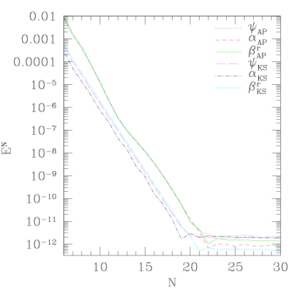
Figure 1: The average error over all collocation points $E^{N}$ as a function of the number of collocation points $N$ for two analytic representations of the Schwarzschild geometry in isotropic coordinates. The label $AP$ denotes the analytic puncture solution presented in Baumgarte and Naculich (2007), while the label $KS$ denotes the Kerr- Schild solution in Cook and Pfeiffer (2004). The errors drop off exponentially as a function of the number of collocation points $N$, until a ‘floor’ of specified tolerance has been reached.

More interesting are the two isotropic representations of the Schwarzschild geometry presented in Cook and Pfeiffer (2004) and Baumgarte and Naculich (2007). The former is a transformation of Kerr-Schild (Eddington-Finkelstein) coordinates to isotropic coordinates, keeping the same time slicing, which we can produce by choosing $K=K_{\rm KS}$ and $\alpha_{\rm AH}=1/\sqrt{2}$ in our code. The latter is an isotropic representation of a maximal slice (with the critical parameter $C=3\sqrt{3}M^{2}/4$, see Estabrook et al. (1973); Reinhart (1973)), which has recently attracted interest as an analytic “puncture” solution (compare Hannam et al. (2006)). We can produce this solution by choosing $K=K_{\rm MS}=0$ and $\alpha_{\rm AH}=3\sqrt{3}/16$ in our code.

To measure the deviation from an analytic solution, we compute the average of the absolute error $\epsilon_{n}$ at all $N$ collocation points in each of the two domains,

$$E^{N}=\frac{1}{2N}\sum_{n=1}^{2N}|\epsilon_{n}|.$$ (34)

where the collocation points $N+1\leq n\leq 2N$ are in the region outside of the shell. In Fig. 1 we graph this error as a function of the number of collocation points $N$. As expected, the errors fall off exponentially for all variables, until they reach a floor corresponding to the predetermined tolerance.

In addition to these vacuum solutions we also consider an analytic solution describing thin shells of non-interacting particles around a static black hole. As we demonstrate in Appendix A, we can solve the differential equations (12) subject to the boundary conditions (14) and (17) as well as the jump conditions (II.3) analytically for maximal slicing and $\alpha_{\rm AH}=0$. As for the solution (33), the field variables become linear in our code’s variables $s_{\rm I}$ and $s_{\rm O}$ (see (36) and (37) below), so that they can be represented exactly for any $N\geq 1$. In addition to testing the solution of the field equations, however, this test also verifies that our code correctly solves the jump conditions at the shell. As in example, we show in Fig. 2 the analytic and numerical solutions for the lapse $\alpha$ and the conformal factor $\psi$ as a function of areal radius $R$ for a Lorentz factor of $W=1.20$ and a mass ratio $M_{BH}/M_{SH}=1$. Our numerical solutions agree with the analytical ones to within better than $10^{-10}$, making them indistinguishable in the plot.

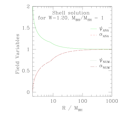
Figure 2: The conformal factor $\psi$ and the lapse $\alpha$ as a function of areal radius for the analytic shell solution ($K=0$ and $\alpha_{\rm EH}=0$) for a Lorentz factor of $W=1.20$ and a mass ratio of $M_{\rm BH}/M_{\rm SH}=1$, corresponding to an areal shell radius of about $8.013M_{\rm BH}$. The field variables are continuous across the shell, but, according to the jump conditions (II.3) their derivatives are not. Our numerical solutions agree with the analytical ones to within better than $10^{-10}$, making the error far smaller than the line width in the graph.

IV Results

Figure 3: The ADM binding energy (29) $E_{\rm B}$ as a function of the shell’s areal radius $R$ for an extreme-mass-ratio sequence with $M_{BH}/M_{SH}=1000$. Values of the horizon lapse $\alpha_{\rm AH}$ range from zero to unity in increments of $0.1$. The graph includes eleven solid lines (representing an evaluation of the binding energy (29) in maximal slicing) and eleven dashed lines (for Kerr-Schild slicing). All 22 lines coincide within our numerical error. We computed these sequences using $N=26$ collocation points in each domain.

We now construct constant-mass sequences, meaning sequences of varying shell radius $r_{\rm SH}$ but constant shell rest mass $M_{\rm SH}$ and black hole irreducible mass $M_{\rm BH}$. Specifically, we focus on “extreme-mass-ratio” sequences with $M_{BH}/M_{\rm SH}=1000$ and equal-mass sequences $M_{\rm BH}/M_{\rm SH}=1$. For both choices of the mass ratio we construct sequences for our two choices of the extrinsic curvature (13), maximal slicing and Kerr-Schild slicing, and for the horizon lapse (17c) ranging from $\alpha_{\rm AH}=0$ to $\alpha_{\rm AH}=1$ in increments of 0.1.

In the following, we will graph the binding energy (29) as a function of the areal radius. Typically, the binding energy $M_{\rm B}$ is only a small fraction of the involved masses, meaning that the relative error in the binding energy is larger than that for the masses – and hence the fields – themselves. We found that, to achieve similar accuracy, the extreme-mass-ratio sequences (for which the binding energy is much smaller than for the equal-mass sequences) required slightly more collocation points than the equal-mass sequences.

In Fig. 3 we show the binding energy for extreme-mass- ratio sequences with $M_{\rm BH}/M_{\rm SH}=1000$. The graph represents 22 plots, corresponding to the eleven different values of $\alpha_{\rm AH}$ and to evaluating the ADM binding energy (29) for both maximal slicing and Kerr-Schild slicing. To within the accuracy of our code, all 22 lines agree with each other, so that they all lie on top of each other and appear as one line in Fig. 3.

The minimum of the binding energy corresponds to the innermost stable circular orbit (ISCO). In the extreme-mass-ratio limit we may neglect the particles’ self-gravity, so that we are effectively solving for a test-particle in the Schwarzschild geometry. As expected, we find that the ISCO is located at $R=6M_{\rm BH}$, representing another independent test of our code.

Figure 4: The ADM binding energy $E_{\rm B}$ as a function of the shell’s areal radius $R$ for an equal mass sequence, $M_{BH}/M_{SH}=1$. As in Fig. 3, values of $\alpha_{\rm AH}$ again range from zero to unity in increments of $0.1$, and the graph again contains eleven lines each for Maximal and Kerr-Schild slicing. All 22 lines again coincide within our numerical error. We obtained these results with $N=20$ collocation points in each domain.

In Fig. 4 we show the equivalent graphs for equal-mass sequences with $M_{\rm BH}/M_{\rm SH}=1$. As for the extreme-mass- ratio sequences in Fig. 3 all 22 graphs coincide to within our numerical accuracy. We note that the ISCO is now located at a larger radius of about $9.367M_{\rm BH}$.

Even in this case, we do not find any evidence that the choice of the slicing condition (13), or the choice of the boundary condition for the lapse on the horizon (17c), have any effect on the physical content of our solutions. Clearly, these different choices lead to different solutions for the conformal factor $\psi$, the lapse $\alpha$ and the shift $\beta$. When expressed in terms of gauge-invariant quantities, however, all our solutions become indistinguishable to within the accuracy of our numerical code.

V Summary

We solve Einstein’s constraint equations in the extended conformal thin-sandwich decomposition to construct spherical shells of non-interacting, isotropic particles in circular orbit about a non-rotating black hole. We construct these solutions for both maximal slicing and Kerr-Schild slicing (see equations (13)), and for a number of different choices for the horizon lapse. These different choices lead to very different solutions for the lapse $\alpha$, the shift $\beta^{i}$ and the conformal factor $\psi$. However, when expressed in terms of gauge-invariant quantities – for example the binding energy as a function of the shell’s areal radius for given shell and black hole masses – our solutions become indistinguishable. At least in the limited context of our spherically symmetric solutions, these findings provide no evidence that the choices for the mean curvature and horizon lapse affect the physical content of the solutions.

Appendix A An analytical solution

For maximal slicing ($K=0$) and the lapse boundary condition $\alpha_{\rm AH}=0$, we can find an analytic solution to the differential equations (12), subject to the boundary conditions (14) and (17) as well as the jump conditions (II.3). The solution depends on the input parameters $M_{\rm SH}$, $W$, $r_{\rm BH}$, and $r_{\rm SH}$. We may then enforce the geodesic condition (24) to eliminate one of these variables, and compute the mass of the black hole from (30). The solution presented here represents a generalization of the solutions of Skoge and Baumgarte (2002), who considered the same system but without a black hole.

We begin with the momentum constraint (12b). For $K=0$ and $\alpha_{\rm AH}=0$ we find that

$$\beta=0$$ (35)

is a self-consistent solution to both the equation and its boundary conditions. This implies that Eqs. (12a) and (12c) for respectively the conformal factor $\psi$ and the combination $\alpha\psi$ reduce to flat Laplace equations in the vacuum regions away from the shell. In spherical symmetry, the only possible solutions are of the form $k_{1}+k_{2}/r$, where $k_{1}$ and $k_{2}$ are arbitrary constants that have to be determined from the boundary conditions. For each function we need four conditions to determine these constants both in the interior and the exterior of the shell. These four conditions arise from the outer boundary conditions (14), the inner boundary conditions (17), continuity of the functions at the shell, and the jump conditions (II.3) for their first derivatives. Using these conditions, we find

$$\psi=\left\{\begin{array}[]{ll}a\left(1+\dfrac{r_{\rm BH}}{r}\right)\,,&r\leq r_{\rm SH}\\[8.53581pt] 1+\dfrac{a\left(r_{\rm SH}+r_{\rm BH}\right)-r_{\rm SH}}{r}\,,&r\geq r_{\rm SH}\end{array}\right.$$ (36)

for the conformal factor and

$$\alpha=\left\{\begin{array}[]{ll}\displaystyle\dfrac{c\left(1-r_{\rm BH}/r\right)}{a\left(1+r_{\rm SH}/r\right)}\,,&r<r_{\rm SH}\\[8.53581pt] \displaystyle\dfrac{1+\left(c\left(r_{\rm BH}-r_{\rm SH}\right)-r_{\rm SH}\right)/r}{1+\left(a\left(r_{\rm SH}+r_{\rm BH}\right)-r_{\rm SH}\right)/r}\,,&r\geq r_{\rm SH}\end{array}\right.$$ (37)

for the lapse. Here the constants $a$ and $c$ are given by

$$a=1+\frac{M_{\rm SH}W}{2r_{\rm SH}\psi_{\rm SH}}$$ (38)

and

$$c=1-\frac{M_{\rm SH}\alpha_{\rm SH}\left(3W^{2}-2\right)}{r_{\rm SH}\left(2W\psi_{\rm SH}\right)}.$$ (39)

Inserting these constants, which themselves depend on the values of the conformal factor and the lapse at the shell, into (36) and (37), we find

$$\psi_{\rm SH}=\frac{1}{2}\left(1+\frac{r_{\rm BH}}{r_{\rm SH}}\right)\left[1+\left(1+\frac{2M_{\rm SH}W}{r_{\rm BH}+r_{\rm SH}}\right)^{1/2}\right]$$ (40)

and

$$\alpha_{\rm SH}=\left(p+\frac{\left(3+p\right)W^{2}-2}{2r_{\rm SH}\psi_{\rm SH}W}\right)^{-1}.$$ (41)

Here we have abbreviated $p\equiv(r_{\rm SH}+r_{\rm BH})/(r_{\rm SH}-r_{\rm BH})$.

So far these solutions depend on all four parameters $M_{\rm SH}$, $W$, $r_{\rm BH}$, and $r_{\rm SH}$. We now find a relation between these parameters by inserting (36) and (37) into the geodesic equation (23), which yields

$$\Omega^{2}=\left(\dfrac{u^{\phi}}{u^{t}}\right)^{2}=-\dfrac{{}^{(4)}\Gamma^{r}_{tt}}{{}^{(4)}\Gamma^{r}_{\phi\phi}}$$ (42)

$$=\dfrac{r_{\rm SH}^{3}c\left(r_{\rm BH}-r_{\rm SH}\right)\left(r_{\rm SH}\left(a-c\right)+r_{\rm BH}\left(a+c+2ac\right)\right)}{2\left(a\left(r_{\rm SH}+r_{\rm BH}\right)\right)^{6}\left(ar_{\rm BH}-r_{\rm SH}\right)}.$$

Unfortunately, this expression is not very useful for our purposes in this form. We find an alternative form by evaluating (24) for our solution (36) and (37), which results in a fifth order polynomial for $W$,

$$0 = 4(r_{\rm BH}-r_{\rm SH})^{3}r_{\rm SH}$$ (43)

$$+M_{\rm SH}(r_{\rm BH}-r_{\rm SH})^{2}(r_{\rm BH}+r_{\rm SH})W$$

$$-2r_{\rm SH}(r_{\rm BH}-r_{\rm SH})(5r_{\rm BH}^{2}-14r_{\rm BH}r_{\rm SH}+5r_{\rm SH}^{2})W^{2}$$

$$-2M_{\rm SH}(r_{\rm BH}-2r_{\rm SH})(r_{\rm BH}-r_{\rm SH})(r_{\rm BH}+r_{\rm SH})W^{3}$$

$$+6r_{\rm SH}(r_{\rm BH}-r_{\rm SH})(r_{\rm BH}^{2}-4r_{\rm BH}r_{\rm SH}+r_{\rm SH}^{2})W^{4}$$

$$+M_{\rm SH}(r_{\rm BH}-2r_{\rm SH})^{2}(r_{\rm BH}+r_{\rm SH})W^{5}$$

In the limit of a zero-mass black hole we have $r_{\rm BH}=0$ and (43) reduces to

$$0 = -4r_{\rm SH}+M_{\rm SH}W+10r_{\rm SH}W^{2}-4M_{\rm SH}W^{3}$$ (44)

$$-6r_{\rm SH}W^{4}+4M_{\rm SH}W^{5},$$

which agrees with the corresponding equation (26) of Skoge and Baumgarte (2002).

Instead of parameterizing the solution by $r_{\rm BH}$, it is more desirable to fix the black hole mass $M_{\rm BH}=M_{\rm irr}$. Towards this end we combine (43) with (36) and (30), which results in a quadratic equation for $r_{\rm SH}$. The solutions to this equation are

$$r_{\rm SH} = \Big{[}4M_{\rm BH}r_{\rm BH}^{2}+2M_{\rm BH}M_{\rm SH}r_{\rm BH}W-2M_{\rm BH}^{2}r_{\rm BH}$$ (45)

$$\pm 2\sqrt{2}\big{(}M_{\rm BH}M_{\rm SH}^{2}r_{\rm BH}^{3}W^{2}\big{)}^{1/2}\Big{]}/$$

$$\Big{[}2(M_{\rm BH}^{2}-2M_{\rm BH}r_{\rm BH})\Big{]}.$$

We henceforth ignore the “$-$” solution, as only the “$+$” solution refers to stable solutions.

Finally, we may insert (45) back into (43), which results into a polynomial for $r_{\rm BH}$ that can be factored into two cubic polynomials

$$0 = \left(a_{3}\bar{r}_{\rm BH}^{3}+a_{2}\bar{r}_{\rm BH}^{2}+a_{1}\bar{r}_{\rm BH}+a_{0}\right)\times$$ (46)

$$\left(b_{3}\bar{r}_{\rm BH}^{3}+b_{2}\bar{r}_{\rm BH}^{2}+b_{1}\bar{r}_{\rm BH}+b_{0}\right).$$

Here we have abbreviated $\bar{r}_{\rm BH}\equiv r_{\rm BH}/M_{\rm SH}$, and the coefficients $a_{i}$ and $b_{i}$ are, in terms of the mass ratio $q\equiv M_{\rm BH}/M_{\rm SH}$,

$$a_{3} = b_{3}=32q^{2}(-2+3W^{2})^{2}$$ (47)

$$a_{2} = -16q(-2+3W^{2})[-4q^{2}+6qW$$

$$+(6q^{2}-1)W^{2}-9qW^{3}+2W^{4}]$$

$$b_{2} = -4q(-2+3W^{2})^{2}(8q^{2}-8qW+5W^{2})$$

$$a_{1} = 2[16q^{4}-48q^{3}W+(44q^{2}-48q^{4})W^{2}$$

$$+(144q^{3}-12q)W^{3}+(36q^{4}-136q^{2}$$

$$+1)W^{4}+(38q-108q^{3})W^{5}+(105q^{2}$$

$$-2)W^{6}-30qW^{7}+W^{8}]$$

$$b_{1} = 2(-2+3W^{2})[-8q^{4}+16q^{3}W$$

$$+(12q^{4}-20q^{2})W^{2}+(10q-24q^{3})W^{3}$$

$$+(26q^{2}-2)W^{4}-12qW^{5}+3W^{6}]$$

$$a_{0} = b_{0}=-qW^{2}(-2q+W+3qW^{2}-2W^{3})^{2}$$

We can now construct a solution for given masses $M_{\rm BH}$ and $M_{\rm SH}$ and Lorentz factor $W$ as follows. Given the mass ratio $q$ and $W$ we first find the six solutions for $\bar{r}_{\rm BH}$ from the two polynomials in (46). We then insert the corresponding values $r_{\rm BH}$ into (45), which yields six solutions for $r_{\rm SH}$. The largest real solution is the solution of interest; we keep only this solution as well as its corresponding value of $r_{\rm BH}$ and disregard all others. These values can then be inserted into (36) and (37), which determines the solution completely.

References

- Darmois (1927) G. Darmois, Mém. Sc. Math. 25, 1 (1927).
- Arnowitt et al. (1962) R. Arnowitt, S. Deser, and C. W. Misner, in Gravitation: an Introduction to Current Research, edited by L. Witten (Wiley, 1962), p. 227.
- York, Jr. (1979) J. W. York, Jr., in Sources of gravitational radiation, edited by L. L. Smarr (Cambridge University Press, Cambridge, 1979), p. 83.
- Pfeiffer (2004) H. P. Pfeiffer, in Proceedings of Miami Waves Conference 2004 (2004), eprint gr-qc/0412002.
- Gourgoulhon (in press) E. Gourgoulhon, in Proceedings of the VII Mexican School on Gravitation and Mathematical Physics, edited by M. Alcubierre (J. Phys.: Conf. Ser., in press), eprint arXiv:0704.0149.
- York, Jr. (1999) J. W. York, Jr., Phys. Rev. Lett. 82, 1350 (1999).
- Pfeiffer and York, Jr. (2003) H. P. Pfeiffer and J. W. York, Jr., Phys. Rev. D 67, 044022 (2003).
- Cook (2000) G. B. Cook, Living Rev. Relat. 5, 1 (2000).
- Baumgarte and Shapiro (2003) T. W. Baumgarte and S. L. Shapiro, Phys. Rept. 376, 41 (2003).
- Cook (2002) G. B. Cook, Phys. Rev. D 65, 084003 (2002).
- Cook and Pfeiffer (2004) G. B. Cook and H. P. Pfeiffer, Phys. Rev. D 70, 104016 (2004).
- Jaramillo et al. (2004) J. L. Jaramillo, E. Gourgoulhon, and G. A. Mena Marugan, Phys. Rev. D 70, 124036 (2004).
- Ashtekar and Krishnan (2004) A. Ashtekar and B. Krishnan, Living Rev. Relat. 7, 10 (2004).
- Dreyer et al. (2003) O. Dreyer, B. Krishnan, D. Shoemaker, and E. Schnetter, Phys. Rev. D 67, 024018 (2003).
- Gourgoulhon and Jaramillo (2006) E. Gourgoulhon and J. L. Jaramillo, Phys. Rept. 423, 159 (2006).
- Skoge and Baumgarte (2002) M. L. Skoge and T. W. Baumgarte, Phys. Rev. D 66, 107501 (2002).
- Gourgoulhon (2007) E. Gourgoulhon, 3+1 formalism and bases of numerical relativity (2007), lectures at the General Relativity Trimester held in Institut Henri Poincaré (Paris, Sept.-Dec. 2006), eprint gr-qc/0703035.
- Beig (1978) R. Beig, Phys. Lett. 69A, 153 (1978).
- Ashtekar and Magnon-Ashtekar (1979) A. Ashtekar and A. Magnon-Ashtekar, J. Math. Phys. 20, 793 (1979).
- Grandclément and Novak (2007) P. Grandclément and J. Novak, Living Rev. Relat. (2007), submitted, eprint arXiv:0706.2286.
- Baumgarte and Naculich (2007) T. W. Baumgarte and S. G. Naculich, Phys. Rev. D 75, 067502 (2007).
- Estabrook et al. (1973) F. Estabrook, H. Wahlquist, S. Christensen, B. Dewitt, L. Smarr, and E. Tsiang, Phys. Rev. D 7, 2814 (1973).
- Reinhart (1973) B. L. Reinhart, J. Math. Phys. 14, 719 (1973).
- Hannam et al. (2006) M. Hannam, S. Husa, B. Bruegmann, J. A. González, U. Sperhake, and N. Ó Murchadha (2006), eprint gr-qc/0612097.