Performance bounds and codes design criteria for channel decoding with a-priori information

Abstract

In this article we focus on the problem of channel decoding in presence of a-priori information. In particular, assuming that the a-priori information reliability is not perfectly estimated at the receiver, we derive a novel analytical framework for evaluating the decoder’s performance. It is derived the important result that a ”good code”, i.e., a code which allows to fully exploit the potential benefit of a-priori information, must associate information sequences with high Hamming weights to codewords with low Hamming weights. Basing on the proposed analysis, we analyze the performance of convolutional codes, random codes, and turbo codes. Moreover, we consider the transmission of correlated binary sources from independent nodes, a problem which has several practical applications, e.g. in the case of sensor networks. In this context, we propose a very simple joint source-channel turbo decoding scheme where each decoder works by exploiting a-priori information given by the other decoder. In the case of block fading channels, it is shown that the inherent correlation between information signals provide a form of non-cooperative diversity, thus allowing joint source-channel decoding to outperform separation-based schemes.

I Introduction

In most digital applications source and channel coding are treated as separate schemes, and the common approach of channel coding is to consider source encoded streams as statistically independent streams. However, in several situations it is not possible, or not convenient, to let source coding eliminating all intrinsic data redundancy. In this cases, the decoder can exploit such a residual (or total) redundancy in its effort of combating noise by performing joint source-channel decoding (JSCD). However, one of the main problem which arises in JSCD is represented by implementation complexity of the decoder, which in general increases to take into account the memory of the information source. As an example, for a first-order Markov source which is protected by convolutional codes, the optimum JSCD scheme is the maximum a posteriori (MAP) sequence decoder based on a super-trellis . The number of the super-trellis states is the product of the number of states of the convolutional trellis and the Markov trellis. Some methods have been proposed to reduce the number of trellis states, which result in suboptimum MAP decoders based on symbol or bit-level [1], [2], [3], [4], [5], [6]. Suboptimal codes aim at presenting redundancy of information sources as a-priori information (API) at the input of channel decoder/demodulator, so that iterative schemes can be easily derived where at each iteration API can be easily enclosed in the decoder without substantially increasing the receiver complexity. In particular, when API is presented at bit-level, the use of channel decoding schemes can be easily extended to all MAP-based decoding schemes, e.g., turbo decoders and LDPC decoders [7], [8].

Another field where JSCD is gaining its momentum is the transmission of detected signals observed at different nodes in Wireless Sensor Networks (WSNs) [9]. In the case of a single collector node (the access point), the study of efficient transmission mechanisms is often referred to as reach-back channel problem [10], [11], [12]. In an attempt to exploit the intrinsic correlation among data, many works have recently focussed on the design of source coding schemes that approach the Slepian-Wolf fundamental limit on the achievable compression rates [13], [14], [15], [16], thus applying the separation principle. However, the design of good practical source codes for correlated sources is still an open problem. Besides, separation between source and channel coding may lead to catastrophic error propagation. Eventually, the traditional code design requires that the correlation between the two sources is known in the encoding process, a requisite that in many applications (e.g., when the nodes are randomly placed in an environment) can be hardly achieved. In an attempt to overcome this impairment, several papers have proposed JSCD schemes where the correlated sources are channel encoded at a reduced rate (with respect to the uncorrelated case). The reduced reliability due to channel coding rate reduction can be compensated by exploiting correlation among different information sources at the channel decoder [17], [18], [19], [20], [21]. In particular, exploiting correlation by means of API has been shown to achieve very good performance.
Although the great attention that has been given to these topics in the recent literature, the problem of designing good codes in presence of API has not been addressed so far. This is because it is generally assumed that good codes in the classical case (no API) are still good in presence of API. In an attempt to fill this lack, in this paper we derive some useful bounds for the bit error probability which establish that the performance depends not only on codewords’ weights, as in traditional decoding, but also on information data weights. The proposed analysis allows to give an insight into the design of good codes, i.e., channel codes which permit to take the best advantage from exploiting API at the decoder. Furthermore, we consider the transmission of correlated binary sources from independent nodes and we propose a very simple JSCD scheme, where each decoder works by exploiting API given by the other decoder.
This paper is structured as follows. In Section II, we derive the pairwise error probability in presence of API at the decoder. In Section III we validate the analysis in the uncoded case. In Section IV we provide an analytical study for evaluating performance in three different coded scenarios: (i) convolutional codes, (ii) random codes with infinite length, and (iii) turbo codes. Eventually, in Section IV we propose a JSCD scheme for decoding correlated binary sources from independent nodes. Finally, concluding remarks are given in Section IV.

II Pairwise error probability evaluation

We consider an i.i.d binary source signal ${\mathbf{x}}$ of length $k$ which is channel encoded with rate $r=k/n$ and denote by ${\mathbf{c}}$ the binary coded signal of length $n$. We assume that a side-information $\tilde{x}_{i}=0/1$ about the message ${\mathbf{x}}$ is available at the decoder and we denote to as $\rho$ the side-information reliability, i.e., $\rho=Pr\left(\tilde{x}_{i}=x_{i}\right)$. Let introduce the a-priori log-likelihood terms $L({{x}}_{i})=ln\left[\frac{Pr\left({{x}}_{i}=0\right)}{Pr\left({{x}}_{i}=1\right)}\right]$ ($ln$ represents the natural logarithm). Given these notations, it is easy to derive $L(x_{i})=L(x)\times(-2\tilde{x}_{i}+1)$, where $L(x)=ln\left(\frac{\rho}{1-\rho}\right)$. Of course, in order to fruitfully exploit the side information, the channel decoder must generate an estimate of the reliability $\rho$. This can be easily obtained by evaluating the number of zeros of the XOR between the received sequences. In the following, we assume that an estimation $\tilde{\rho}$ is available at the decoder. Accordingly, we introduce $\tilde{L}(x)=ln\left(\frac{\tilde{\rho}}{1-\tilde{\rho}}\right)$.
Let us denote by ${\mathbf{y}}({\mathbf{x}})$ the transmitted signal and assume a binary antipodal modulation scheme, so that ${\mathbf{y}}({\mathbf{x}})=-2{\mathbf{c}}({\mathbf{x}})+1$. Eventually, assuming an AWGN channel model, we can express the received signal ${\mathbf{z}}$ as:

$$\begin{array}[]{cl}{\mathbf{z}}=\sqrt{2r\xi_{b}}\times{\mathbf{y}}({\mathbf{x}})+{\mathbf{\eta}}\end{array}$$ (1)

where $\eta_{i}$ are Gaussian random noise terms with zero mean and variance $N_{0}$ and $\xi_{b}$ is the energy per bit.
Denoting by $\tilde{{\mathbf{x}}}$ the side information at the decoder, the MAP decoding rule can be expressed as:

$$\begin{array}[]{cl}\hat{{\mathbf{x}}}=\mathop{arg~{}max}\limits_{{{\mathbf{x}}}}~{}\Pr\left\{{\mathbf{x}}|\tilde{\rho},\tilde{{{\mathbf{x}}}},{{\mathbf{z}}}\right\}\end{array}$$ (2)

By using the Bayes’ rule and neglecting any constant term (i.e., the terms which do not depend on ${{\mathbf{x}}}$), it is now straightforward to get from (2) the equivalent decoding rule:

$$\begin{array}[]{cl}\hat{{\mathbf{x}}}=\mathop{arg~{}max}\limits_{{{\mathbf{x}}}}~{}\Pr\left\{{{\mathbf{z}}}|{\mathbf{x}}\right\}Pr\left\{{{\mathbf{x}}}|\tilde{\rho},\tilde{{{\mathbf{x}}}}\right\}\end{array}$$ (3)

Using the AWGN assumption and substituting for ${{\mathbf{z}}}$ the expression given in (1) it is easy to derive:

$$\begin{array}[]{cl}\tilde{{\mathbf{x}}}=\mathop{arg~{}max}\limits_{{{\mathbf{x}}}}\left[\sqrt{2r\xi_{b}}\sum\limits_{i=0}^{n-1}z_{i}y_{i}+N_{0}\times ln\left(Pr\left\{{{\mathbf{x}}}|\tilde{\rho},\tilde{{{\mathbf{x}}}}\right\}\right)\right]\end{array}$$ (4)

Let us now denote by ${{\mathbf{x}}_{t}}$ the transmitted information signal, and by ${{\mathbf{x}}_{e}}\neq{{\mathbf{x}}_{t}}$ the estimated sequence. Moreover, let denote by ${{\mathbf{y}}_{e}}\neq{{\mathbf{y}}_{t}}$ the corresponding codewords. The pairwise error probability conditioned to $\tilde{{{\mathbf{x}}}}$ can be defined as the probability that the metric (4) evaluated for ${\mathbf{y}}={{\mathbf{y}}_{e}}$ and ${\mathbf{x}}={{\mathbf{x}}_{e}}$ is higher than that evaluated for ${\mathbf{y}}={{\mathbf{y}}_{t}}$ and ${\mathbf{x}}={{\mathbf{x}}_{t}}$. Such a probability can be expressed as:

$$\begin{array}[]{cl}P_{e}\left({{\mathbf{x}}_{t}},{{\mathbf{x}}_{e}}|\tilde{{{\mathbf{x}}}}\right)=\Pr\left\{\sqrt{2r\xi_{b}}\sum\limits_{i=0}^{n-1}z_{i}\left(y_{i,e}-y_{i,t}\right)-N_{0}\times ln\left(\frac{Pr\left\{{{\mathbf{x}}_{t}}|\tilde{\rho},\tilde{{{\mathbf{x}}}}\right\}}{Pr\left\{{{\mathbf{x}}_{e}}|\tilde{\rho},\tilde{{{\mathbf{x}}}}\right\}}\right)>0\right\}\end{array}$$ (5)

Substituting for ${\mathbf{z}}$ in (5) the expression given in (1), it is straightforward to obtain:

$$\begin{array}[]{cl}P_{e}\left({{\mathbf{x}}_{t}},{{\mathbf{x}}_{e}}|\tilde{{{\mathbf{x}}}}\right)=0.5erfc\left[\sqrt{rd\gamma_{b}}+\frac{1}{4\sqrt{rd\gamma_{b}}}ln\left(\frac{Pr\left\{{{\mathbf{x}}_{t}}|\tilde{\rho},\tilde{{{\mathbf{x}}}}\right\}}{Pr\left\{{{\mathbf{x}}_{e}}|\tilde{\rho},\tilde{{{\mathbf{x}}}}\right\}}\right)\right]\end{array}$$ (6)

where $\gamma_{b}=\frac{\xi_{b}}{N_{0}}$, $d=D\left({{\mathbf{c}}_{t}},{{\mathbf{c}}_{e}}\right)$ is the Hamming distance between ${{\mathbf{c}}_{t}}$ and ${{\mathbf{c}}_{e}}$ and $erfc$ is the complementary error function.

To elaborate, we get from the hypothesis that ${{{\mathbf{x}}}}$ is an i.i.d. sequence:

$$\begin{array}[]{cl}\frac{Pr\left\{{{\mathbf{x}}_{t}}|\tilde{\rho},\tilde{{{\mathbf{x}}}}\right\}}{Pr\left\{{{\mathbf{x}}_{e}}|\tilde{\rho},\tilde{{{\mathbf{x}}}}\right\}}=\prod\limits_{i=0}^{k-1}\frac{Pr\left\{{{{x}}_{i,t}}|\tilde{\rho},\tilde{{{{x}}}}_{i}\right\}}{Pr\left\{{{{x}}_{i,e}}|\tilde{\rho},\tilde{{{{x}}}}_{i}\right\}}\end{array}$$ (7)

Let us introduce the sequences ${\epsilon}_{i,t}={x}_{i,t}\bigoplus\tilde{x}_{i}$ and ${\epsilon}_{i,e}={x}_{i,e}\bigoplus\tilde{x}_{i}$, where $\bigoplus$ is the bit-wise XOR operator. By exploiting the API $\tilde{{{{x}}}}_{i}$ and its estimated reliability $\tilde{\rho}$, the $i$-th term in (7) can be further elaborated as:

$$\begin{array}[]{cl}\frac{Pr\left\{{{{x}}_{i,t}}|\tilde{\rho},\tilde{{{{x}}}}_{i}\right\}}{Pr\left\{{{{x}}_{i,e}}|\tilde{\rho},\tilde{{{{x}}}}_{i}\right\}}=\frac{\tilde{\rho}^{{\epsilon}_{i,t}}\times\left(1-\tilde{\rho}\right)^{\bar{{\epsilon}}_{i,t}}}{\tilde{\rho}^{{\epsilon}_{i,e}}\times\left(1-\tilde{\rho}\right)^{\bar{{\epsilon}}_{i,e}}}=\left\{\begin{array}[]{ccccc}1&if&{{{x}}_{i,t}}={{{x}}_{i,e}}&{}\hfil&{}\hfil\\ \frac{\tilde{\rho}}{1-\tilde{\rho}}&if&{{{x}}_{i,t}}\neq{{{x}}_{i,e}}&and&{{{\epsilon}}_{i,t}}=0\\ \frac{1-\tilde{\rho}}{\tilde{\rho}}&if&{{{x}}_{i,t}}\neq{{{x}}_{i,e}}&and&{{{\epsilon}}_{i,t}}=1\end{array}\right.\end{array}$$ (8)

where $\bar{{\epsilon}}_{i,t}$ and $\bar{{\epsilon}}_{i,e}$ are the NOT version of ${{\epsilon}}_{i,t}$ and ${{\epsilon}}_{i,e}$, respectively. Hence, denoting by $U\left({{\mathbf{x}}_{t}},{{\mathbf{x}}_{e}}\right)$ the set of indexes such as ${{{x}}_{i,t}}\neq{{{x}}_{i,e}}$, i.e., ${{{x}}_{i,t}}\neq{{{x}}_{i,e}}$ $\forall$ $i\in U\left({{\mathbf{x}}_{t}},{{\mathbf{x}}_{e}}\right)$, we can write:

$$\begin{array}[]{cl}\frac{Pr\left\{{{\mathbf{x}}_{t}}|\tilde{\rho},\tilde{{{\mathbf{x}}}}\right\}}{Pr\left\{{{\mathbf{x}}_{e}}|\tilde{\rho},\tilde{{{\mathbf{x}}}}\right\}}=\prod\limits_{i\in U\left({{\mathbf{x}}_{t}},{{\mathbf{x}}_{e}}\right)}\frac{Pr\left\{{{{x}}_{i,t}}|\tilde{\rho},\tilde{{{{x}}}}_{i}\right\}}{Pr\left\{{{{x}}_{i,e}}|\tilde{\rho},\tilde{{{{x}}}}_{i}\right\}}\end{array}$$ (9)

For the sake of notation clarity, we assume without loss of generality that $U\left({{\mathbf{x}}_{t}},{{\mathbf{x}}_{e}}\right)$ is the set $\{0,1,\ldots,w-1\}$, $w$ being the cardinality of $U\left({{\mathbf{x}}_{t}},{{\mathbf{x}}_{e}}\right)$, i.e., $w=D\left({{\mathbf{x}}_{t}},{{\mathbf{x}}_{e}}\right)$ is the Hamming distance between ${{\mathbf{x}}_{t}}$ and ${{\mathbf{x}}_{e}}$. Hence, we can write from (8) and (9):

$$\begin{array}[]{cl}\frac{Pr\left\{{{\mathbf{x}}_{t}}|\tilde{\rho},\tilde{{{\mathbf{x}}}}\right\}}{Pr\left\{{{\mathbf{x}}_{e}}|\tilde{\rho},\tilde{{{\mathbf{x}}}}\right\}}=\left(\frac{\tilde{\rho}}{1-\tilde{\rho}}\right)^{w-\sum\limits_{i=0}^{w-1}{\epsilon}_{i,t}}\times\left(\frac{1-\tilde{\rho}}{\tilde{\rho}}\right)^{\sum\limits_{i=0}^{w-1}{\epsilon}_{i,t}}=\left(\frac{\tilde{\rho}}{1-\tilde{\rho}}\right)^{w-\sum\limits_{i=0}^{w-1}{2\epsilon}_{i,t}}\end{array}$$ (10)

Denoting for the sake of simplicity ${\epsilon}_{i,t}={\epsilon}_{i}$, remembering that $\tilde{L}(x)=ln\left(\frac{\tilde{\rho}}{1-\tilde{\rho}}\right)$, and introducing the term $\tilde{w}=\sum\limits_{i=0}^{w-1}{\epsilon}_{i}$, it is now straightforward to rewrite (6) as:

$$\begin{array}[]{cl}P_{e}\left({{\mathbf{x}}_{t}},{{\mathbf{x}}_{e}}|\tilde{{{\mathbf{x}}}}\right)=0.5erfc\left(\sqrt{{rd\gamma_{b}}\left(1+\frac{1}{d}\frac{\tilde{L}(x)(w-2\tilde{w})}{4r\gamma_{b}}\right)^{2}}\right)\end{array}$$ (11)

It can be observed from (11) that, if we condition to $\tilde{w}$, the pairwise error probability depends on $d$ and $w$ rather than on the whole transmitted and estimated sequences ${{\mathbf{x}}_{t}}$ and ${{\mathbf{x}}_{e}}$. It is then possible to write:

$$\begin{array}[]{cl}P_{e}\left(d,w|\tilde{w}\right)=0.5erfc\left(\sqrt{{rd\gamma_{b}}\left(1+\frac{1}{d}\frac{\tilde{L}(x)(w-2\tilde{w})}{4r\gamma_{b}}\right)^{2}}\right)\end{array}$$ (12)

Note that, according to the correlation model, ${\epsilon}_{i}$ are i.i.d binary random term with $Pr\left\{{\epsilon}_{i}=0\right\}=\rho$ and $Pr\left\{{\epsilon}_{i}=1\right\}=1-\rho$. Hence, $\tilde{w}$ is binomially distributed with parameters $w$ and $1-\rho$, and the pairwise error probability can be eventually derived as:

$$\begin{array}[]{cl}P_{e}\left(d,w\right)=0.5\sum\limits_{\tilde{w}=0}^{w}erfc\left(\sqrt{{rd\gamma_{b}}\left(1+\frac{1}{d}\frac{\tilde{L}(x)(w-2\tilde{w})}{4r\gamma_{b}}\right)^{2}}\right){w\choose\tilde{w}}\rho^{w-\tilde{w}}\times(1-\rho)^{\tilde{w}}\end{array}$$ (13)

The above expression is quite messy to manipulate. A significant simplification occurs if we consider the following bound:

$$\begin{array}[]{c}\left(1+\frac{1}{d}\frac{\tilde{L}(x)\left(w-2\tilde{w}\right)}{4r\gamma_{b}}\right)^{2}\geq 1+\frac{2}{d}\frac{\tilde{L}(x)\left(w-2\tilde{w}\right)}{4r\gamma_{b}}\end{array}$$ (14)

which is a tight lower bound for $rd\gamma_{b}>>|\tilde{L}(x)\left(w-2\tilde{w}\right)|$ , i.e., when the error probability is mainly determined by the codewords’ distance rather than by the beneficial effect of API. In this case, we get:

$$\begin{array}[]{cl}P_{e}\left(d,w\right)\leq 0.5\sum\limits_{\tilde{w}=0}^{w}erfc\left(\sqrt{{rd\gamma_{b}}+\frac{\tilde{L}(x)(w-2\tilde{w})}{2}}\right){w\choose\tilde{w}}\rho^{w-\tilde{w}}\times(1-\rho)^{\tilde{w}}\end{array}$$ (15)

To get the desirable simplification, consider now the Chernoff-Rubin bound for the $erfc$ function, i.e.:

$$\begin{array}[]{c}erfc(x)\leq 2e^{-x^{2}}\end{array}$$ (16)

Accordingly, we can write:

$$\begin{array}[]{c}P_{e}\left(d,w\right)\leq e^{-rd\gamma_{b}}e^{-\frac{\tilde{L}(x)w}{2}}\sum\limits_{\tilde{w}=0}^{w}e^{\tilde{L}(x)\tilde{w}}\times{w\choose\tilde{w}}\rho^{w-\tilde{w}}\times(1-\rho)^{\tilde{w}}\end{array}$$ (17)

which yields:

$$\begin{array}[]{c}P_{e}\left(d,w\right)\leq e^{-rd\gamma_{b}}e^{-\frac{\tilde{L}(x)w}{2}}\left[(1-\rho)e^{\tilde{L}(x)}+\rho\right]^{w}\end{array}$$ (18)

Since $e^{\tilde{L}(x)/2}=\sqrt{\frac{\tilde{\rho}}{1-\tilde{\rho}}}$, if we introduce the term:

$$\begin{array}[]{c}A=(1-\rho)\sqrt{\frac{\tilde{\rho}}{1-\tilde{\rho}}}+\rho\sqrt{\frac{1-\tilde{\rho}}{\tilde{\rho}}}\end{array}$$ (19)

it is straightforward to get from (18):

$$\begin{array}[]{c}P_{e}\left(d,w\right)\leq e^{-rd\gamma_{b}}A^{w}\end{array}$$ (20)

The above expressions allows to separate the influence of signal to noise ratio and codewords distance $d$ (first part) from the effect of API (second part). A more precise measure of the pairwise error probability can be derived by considering the exact evaluation of the first term in (20) instead of its exponential bound, i.e.:

$$\begin{array}[]{c}P_{e}\left(d,w\right)\simeq 0.5erfc\left(\sqrt{rd\gamma_{b}}\right)A^{w}\end{array}$$ (21)

Note that (21) gives an exact calculation of the pairwise error probability for $\rho=\tilde{\rho}=0.5$, i.e., in absence of API. Even if (21) is not a strict bound for $P_{e}\left(d,w\right)$, we will prove by simulations that it gives a quite close upper bound in most of the situations.
Equations (20) and (21) give rise to interesting considerations about the properties of good channel codes in presence of API. As in traditional codes’ design, a good code must be characterized by a high minimum Hamming weight $d$. Moreover, in order to fully exploit the benefits of API, the code structure should allow to associate information sequences with high Hamming weights $w$ to codewords with low Hamming weights $d$. This result can be easily understood if we rewrite (20) as:

$$\begin{array}[]{c}P_{e}\left(d,w\right)\leq e^{-{rd\gamma_{b}}}e^{-{r\gamma_{b}}ln\left({\frac{1}{A}}\right)\times w\frac{1}{r\gamma_{b}}}=\left(e^{-{r\gamma_{b}}}\right)^{d+w\times ln\left({\frac{1}{A}}\right)\frac{1}{r\gamma_{b}}}\end{array}$$ (22)

and if we observe that for reasonable $\rho$ estimates, i.e., $\rho\cong\tilde{\rho}$, we get $A<1$. Hence, denoting by $\alpha=ln\left({\frac{1}{A}}\right)\frac{1}{r\gamma_{b}}$, a rule of the thumb for designing good codes is that of maximizing the minimum $d+w\alpha$ (with $\alpha>0$). Of course, a rigorous analysis should consider the trade-off between diminishing the pairwise error probability from one side and increasing the number of bits in errors $w$ from the other side.

III Uncoded Communications

In the uncoded case $r=k=n=1$, $d=w=1$ and the pairwise error probability is equivalent to the bit error probability, which can be derived according to (13) as:

$$\begin{array}[]{cl}P_{e}=0.5erfc\left(\sqrt{{\gamma_{b}}\left(1+\frac{\tilde{L}(x)}{4\gamma_{b}}\right)^{2}}\right)\rho+0.5erfc\left(\sqrt{{\gamma_{b}}\left(1-\frac{\tilde{L}(x)}{4\gamma_{b}}\right)^{2}}\right)\times(1-\rho)\end{array}$$ (23)

The approximation (21) can be written in this case as:

$$\begin{array}[]{c}P_{e,b}\left(d,w\right)\simeq 0.5erfc\left(\sqrt{\gamma_{b}}\right)A\end{array}$$ (24)

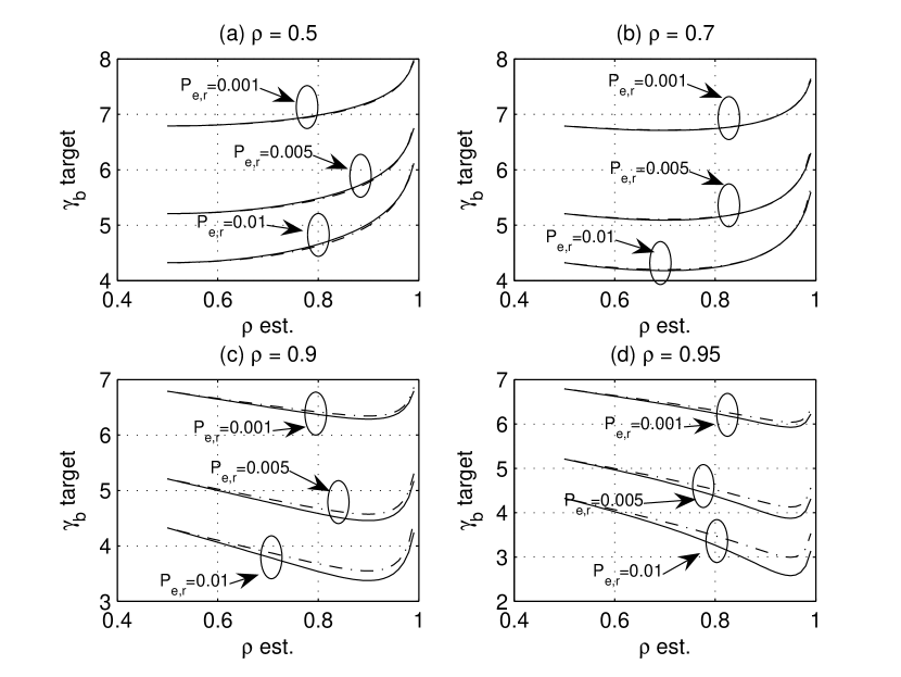
Figure 1: $\gamma_{b}$ required to achieve $P_{e,r}$ versus the estimated $\rho$ (i.e., ${\tilde{\rho}}$ is in the abscissa) in the uncoded case: comparisons between exact calculation (straight lines) and $P_{e,b}$ (dashed lines), for: (a) $\rho=0.5$, (b) $\rho=0.7$, (c) $\rho=0.9$, (a) $\rho=0.95$.

A comparison between the exact calculation in (23) and the approximation in (24) is given in Fig. 1. In the y-axis we report the $\gamma_{b}$ required to achieve a target bit error probability, say it $P_{e,r}$. In the x-axis we report $\tilde{\rho}$. Four different $\rho$ values have been considered, namely $\rho=0.5$ in Fig. 1 (a), $\rho=0.7$ in Fig. 1 (b), $\rho=0.9$ in Fig. 1 (c) and $\rho=0.95$ in Fig. 1 (d). We note that approximation (24) is almost exact for $\rho<0.7$. Moreover, it is a very close upper bound for $\rho>0.7$ and for $P_{e,r}=0.001$, i.e., for high signal to noise ratios. As expected, (24) gives a worse approximation for $\rho=0.9$, $\rho=0.95$ and for $\gamma_{b}<4$, where the bound (14) is less tight. However, also in these cases, (24) gives a quite close upper bound for the bit error probability evaluation. Hence, the proposed approximation allows to give a very good measure of the performance gain which can be obtained by exploiting API at the receiver, even in presence of imperfect estimation. Note that the system performance is quite robust to imperfect reliability estimation, at least for $\rho\leq 0.95$. As an example, for $\rho=0.9$ and $P_{e,r}=0.001$, an estimation of $\tilde{\rho}=0.8$ reduces the performance by only 0.1 dB with respect to perfect estimation ($\tilde{\rho}=0.9$), while an estimation of $\tilde{\rho}=0.95$ reduces the performance by less than 0.08 dB. To sum up, results in Fig. 1 show that API allows to achieve reasonable performance gains at low $\gamma_{b}$ with respect to the $\tilde{\rho}=0.5$ case. This is true even in presence of not very accurate estimation of the side information reliability $\rho$.

IV Coded Communication Schemes

IV-A Convolutional codes

Convolutional coding schemes [22], [23] allow an easy coding implementation with very low power and memory requirements and, hence, they seem to be particularly suitable for utilization in WSNs [24]. Moreover, as stated in the Introduction, correlation among sources may be directly converted to API at the receiver. Hence, optimum decoding schemes can be easily derived by including the a-priori probabilities in the branch metrics of the Viterbi algorithm according to equation (4).
As in traditional convolutional coding (i.e., without API), it is possible to derive an upper bound of the bit error probability as the weighted sum of the pairwise error probabilities relative to all paths which diverge from the zero state and marge again after a certain number of transitions [22]. This is possible because of the linearity of the code and because the pairwise error probability (13) depends only on the weights $d$ and $w$, and not on the actual transmitted sequence.
In particular, it is possible to evaluate the input-output transfer function $T(W,D)$ by means of the state transition relations over the modified state diagram [22]. The generic form of $T(W,D)$ is:

$$\begin{array}[]{cl}T(W,D)=\sum\limits_{w,d}\beta_{w,d}W^{w}D^{d}\end{array}$$ (25)

where $\beta_{w,d}$ denotes the number of paths that start from the zero state and reemerge with the zero state and that are associated with an input sequence of weight $w$, and an output sequence of weight $d$. Accordingly, we can get an upper bound of the bit error probability as:

$$\begin{array}[]{cl}{P}_{e,b}\leq\sum\limits_{w,d}\beta_{w,d}\times w\times{P}_{e}\left(d,w\right)\end{array}$$ (26)

where $P_{e}(d,w)$ is the pairwise error probability. Let now denote by $P_{e,e}$ the exact pairwise error probability derived in (13) and by $P_{e,a}$ the approximation (21). Accordingly, we get the following bound for the bit error probability:

$$\begin{array}[]{cl}{P}_{e,1}=\sum\limits_{w,d}\beta_{w,d}\times w\times{P}_{e,e}\left(d,w\right)\end{array}$$ (27)

A second bound can be obtained by considering the loose upper bound (20):

$$\begin{array}[]{cl}{P}_{e,2}=\sum\limits_{w,d}\beta_{w,d}\times w\times e^{-rd\gamma_{b}}A^{w}\end{array}$$ (28)

From (25) and (28) it is straightforward to obtain:

$$\begin{array}[]{cl}{P}_{e,2}=A\times\frac{\partial T(W,D)}{\partial W}|_{W=A,D=e^{-r\gamma_{b}}}\end{array}$$ (29)

Since ${P}_{e,2}$ is a monotone decreasing function of $\gamma_{b}$, it is straightforward to carry out numerical inversion of $(\ref{eq13AA25})$ with respect to $\gamma_{b}$. Such an inversion allows to get an estimation of the threshold signal-to-noise ratio $\gamma_{b}(P_{e,r},A)$ corresponding to a given ${P}_{e,2}=P_{e,r}$. Note that $\gamma_{b}(P_{e,r},1)$ corresponds to the threshold $\gamma_{b}$ when no API is present at the receiver. Accordingly, the signal-to-noise-ratio gain due to API can be derived as:

$$\begin{array}[]{cl}\Delta P=\frac{\gamma_{b}(P_{e,r},1)}{\gamma_{b}(P_{e,r},A)}\end{array}$$ (30)

In order to assess the validity of the previous analysis, we have carried out computer simulations for both recursive and non-recursive convolutional codes. In both cases, we have considered a rate $r=0.5$ and a constraint length $K=4$. Hence, the codes can be univocally characterized by the generator polynomials $G^{(1)}(D)=g^{(1)}_{3}D^{3}+g^{(1)}_{2}D^{2}+g^{(1)}_{1}D+g^{(1)}_{0}$, $G^{(2)}(D)=g^{(2)}_{3}\times D^{3}+g^{(2)}_{2}D^{2}+g^{(2)}_{1}D+g^{(2)}_{0}$ and by the feedback polynomial $H(D)=h_{3}\times D^{3}+h_{2}D^{2}+h_{1}D+h_{0}$. As for the non-recursive code we have considered the maximum $d_{free}$ code which is optimum in the uncorrelated scenario [23], i.e., $G^{(1)}(D)=D^{3}+D^{2}+1$, $G^{(2)}(D)=D^{3}+D^{2}+D+1$ and, of course, $H(D)=1$. Such a code is characterized by a transfer function:

$$\begin{array}[]{cl}T(D,W)=\frac{D^{6}W^{2}+D^{7}W-D^{8}W^{2}}{1-2DW-D^{3}W}=D^{6}W^{2}+D^{7}W+2D^{7}W^{3}+\ldots\end{array}$$ (31)

It is worth noting that the non-recursive code is characterized by a path with minimum distance $d_{free}=6$ and information weight $w=2$.
As for the recursive code, we consider the generator polynomials $G^{(1)}(D)=D^{3}+D+1$, $G^{(2)}(D)=D^{3}+D^{2}+D+1$ and $H(D)=D^{3}+D^{2}+1$. Such a code is characterized by a transfer function:

$$\begin{array}[]{cl}T(D,W)=\frac{D^{6}W^{2}(D^{6}W^{4}-2D^{6}W^{2}+D^{6}+D^{5}W-D^{5}W^{3}+2W^{4}D^{2}-2D^{2}W^{2}-D^{2}W^{6}+DW^{5}-2DW^{3}+2DW+W^{2})}{1-D^{8}W^{4}+2D^{8}W^{2}-D^{8}-D^{7}W+D^{7}W^{3}-D^{5}W+D^{5}W^{3}+D^{4}W^{2}-2D^{4}W^{4}+D^{4}W^{6}-D^{3}W^{5}+2W^{3}D^{3}-2D^{3}W-2DW}=\\ =D^{6}W^{4}+D^{7}W^{7}+2D^{7}W^{3}+\ldots\end{array}$$ (32)

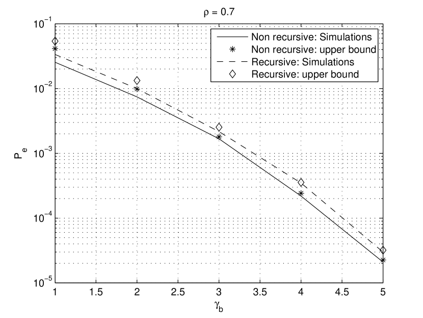
Figure 2: $P_{e}$ versus $\gamma_{b}$ comparisons between recursive and non recursive convolutional codes: simulation results are shown together with the ${P}_{e,1}$ upper bounds for $\rho=0.7$

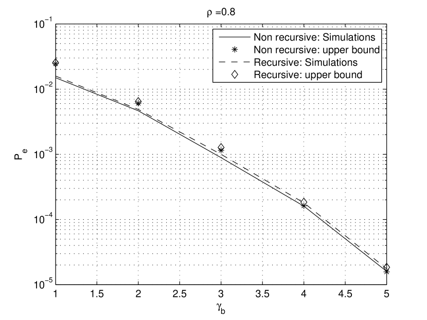
Figure 3: $P_{e}$ versus $\gamma_{b}$ comparisons between recursive and non recursive convolutional codes: simulation results are shown together with the ${P}_{e,1}$ upper bounds for $\rho=0.8$

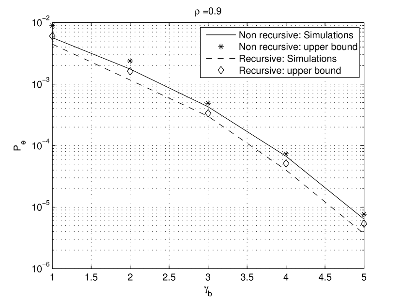
Figure 4: $P_{e}$ versus $\gamma_{b}$ comparisons between recursive and non recursive convolutional codes: simulation results are shown together with the ${P}_{e,1}$ upper bounds for $\rho=0.9$

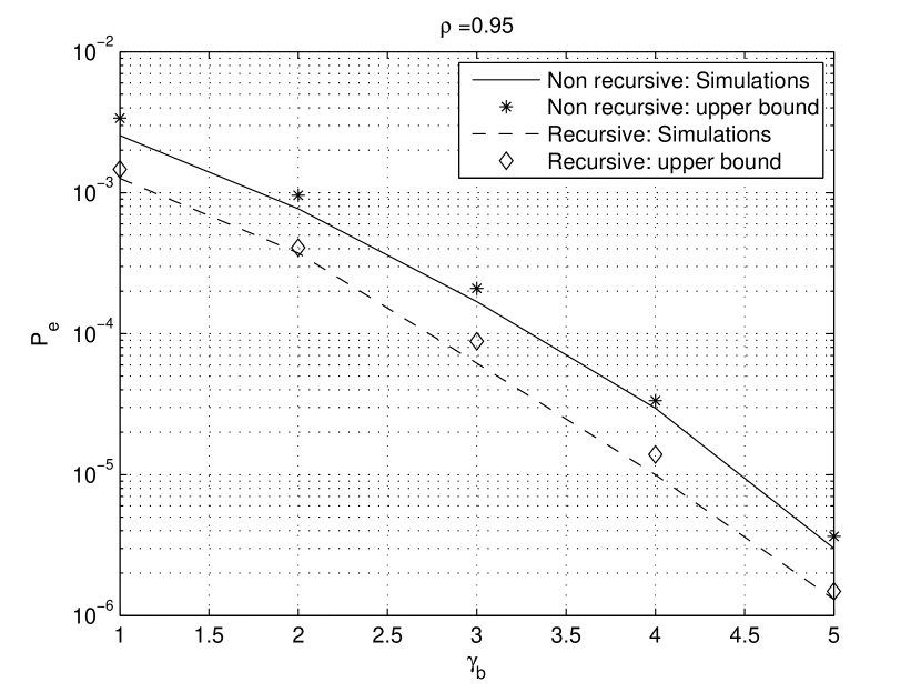
Figure 5: $P_{e}$ versus $\gamma_{b}$ comparisons between recursive and non recursive convolutional codes: simulation results are shown together with the ${P}_{e,1}$ upper bounds for $\rho=0.95$

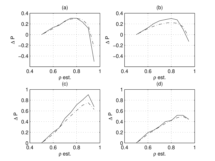
Figure 6: $\Delta P$ versus the estimated $\rho$ (i.e., ${\tilde{\rho}}$ is in the abscissa) for ${P}_{e,r}=0.0001$: comparisons between simulations (straight lines) and analysis in (30) (dashed lines), for: (a) $\rho=0.8$, recursive code (b) $\rho=0.8$, non recursive code (c) $\rho=0.9$, recursive code (d) $\rho=0.9$, non recursive code .

The recursive code is characterized by a path with minimum distance $d_{free}=6$ and information weight $w=4$.
Given the above, for high signal to noise ratios the bit error probability can be approximated as $P_{e}\cong A^{2}erfc\left(\sqrt{3\gamma_{b}}\right)$ for the non-recursive code and as $P_{e}\cong 2A^{4}erfc\left(\sqrt{3\gamma_{b}}\right)$ for the recursive code. Accordingly, we expect that the recursive code outperforms the non-recursive one for $A<\frac{1}{\sqrt{2}}$. Under the hypothesis of perfect reliability estimation, i.e., $\rho=\tilde{\rho}$, this means that the recursive code performs better for $\rho>0.85$.
Comparisons between the above codes are shown in Figs. 2-5 in the case of perfect reliability estimation and for different $\rho$ values, namely $\rho=0.7$ in Fig. 2, $\rho=0.8$ in Fig. 3, $\rho=0.9$ in Fig. 4 and $\rho=0.95$ in Fig. 5. In all figures simulation results are shown together with the ${P}_{e,1}$ upper bound derived in (27).
As one can observe, the analytical upper bound derived in ${P}_{e,1}$ is quite tight and, in particular, tends to perfectly match simulation results for high signal to noise ratios. Moreover, as expected, the recursive code clearly outperforms the non-recursive one for $\rho\geq 0.9$, while for $\rho<0.8$ the non recursive code performs better.
More extensive comparisons between simulations and theoretical analysis have been carried out to evaluate the signal to noise ratio gain $\Delta P$ which can be obtained by means of API at the receiver. Such results are shown in Fig. 6, where $\Delta P$ versus ${\tilde{\rho}}$ for ${P}_{e,r}=0.0001$ is shown. Simulation results are the straight lines while analytical results derived according to (30) are the dashed lines. Different $\rho$ values have been considered, namely $\rho=0.8$ in Figs. 6 (a) and 6 (b) and $\rho=0.9$ in Figs. 6 (c) and 6 (d). Eventually, results for the recursive code are shown in Figs. 6 (a) and 6 (c) and results for the non recursive code are shown in Figs. 6 (b) and 6 (d). We note that approximation (29) allows to predict quite well the beneficial effect of a priori information even in the case of non perfect $\rho$ estimation. It is worth noting that, as expected, recursive code takes grater advantage from exploiting a priori information than non recursive code. As an example, for $\rho=0.9$ the maximum performance gain (i.e., the performance gain which is obtained for $\rho={\tilde{\rho}}$) is 0.9 dB for the recursive code and 0.5 dB for the non recursive code. On the other hand, the recursive code is much more sensitive to estimation errors than the non recursive code (on account of the higher minimum $w$).

IV-B Random Selection Of Codes

In an attempt to derive a general framework for the evaluation of the impact of API in the performance of coded signals, we now consider random selection of codes and we evaluate a bound on the average bit error probability. In the proposed approach we extend the considerations made in [23], Section 7-2, to the case of a priori information at the receiver. In particular, denoting by $M=2^{k}$, we consider the ensemble of $(2^{n})^{M}$ distinct ways in which we can select $M$ binary codewords from the available $2^{n}$ words of length $n$. Each code selection leads to a different communication system which is characterized by its probability of error. As done in [23] we assume that the choice of $M$ codewords is based on random selection. In particular, in [23] it is derived an upper bound on the expected pairwise error probability for a given Hamming distance $d$ as:

$$\begin{array}[]{c}\overline{P_{e}}\leq\frac{1}{2^{n}}\sum\limits_{d=0}^{n}{n\choose d}e^{-rd\gamma_{b}}\\ \end{array}$$ (33)

where the average is evaluated over the ensemble of $(2^{n})^{M}$ codes. Let now consider the upper bound derived in (20) for the pairwise error probability in presence of API. It is worth noting that in this case the pairwise error probability depends on $d$ and $w$, whereas in absence of API it depends only on $d$. Moreover, since the code selection is random, $d$ and $w$ are binomial independent random discrete variables. Hence, averaging over the ensemble of $(2^{n})^{M}$ codes we get in this case:

$$\begin{array}[]{c}\overline{P_{e}}\leq\frac{1}{2^{n}}\frac{1}{2^{k}}\sum\limits_{d=0}^{n}\sum\limits_{w=0}^{k}{n\choose d}{k\choose w}\left(e^{-r\gamma_{b}}\right)^{d}A^{w}\end{array}$$ (34)

where $A$ is defined in (19). From the above, it is then straightforward to derive:

$$\begin{array}[]{c}\overline{P_{e}}\leq\left(\frac{1+e^{-r\gamma_{b}}}{2}\right)^{n}\times\left(\frac{1+A}{2}\right)^{k}\end{array}$$ (35)

Eventually, since the average pairwise error probability is independent of $d$ and $w$ we can easily obtain an union bound on the average bit error probability by considering the sum of all the $M-1$ possible error events, i.e.:

$$\begin{array}[]{c}\overline{P_{e,b}}\leq(M-1)\left(\frac{1+e^{-r\gamma_{b}}}{2}\right)^{n}\times\left(\frac{1+A}{2}\right)^{k}<M\left(\frac{1+e^{-r\gamma_{b}}}{2}\right)^{n}\times\left(\frac{1+A}{2}\right)^{k}\end{array}$$ (36)

This result can be expressed in a more convenient form by introducing the terms $R_{1}={log_{2}\left(\frac{2}{1+e^{-r\gamma_{b}}}\right)}$ and $\eta={log_{2}\left(\frac{2}{1+A}\right)}$. Accordingly, since $M=2^{k}$ and $r=k/n$, (36) becomes:

$$\begin{array}[]{c}\overline{P_{e,b}}<2^{nr-nR_{1}-nr\eta}=2^{-n\left[R_{1}-r(1-\eta)\right]}\end{array}$$ (37)

We have thus obtained a similar expression for the average bit error probability as that in [23], with the introduction of the term $\eta$ which takes into account the effect of API. Hence, introducing the cutoff rate $R_{0}=\frac{R_{1}}{1-\eta}$ we conclude that when $r<R_{0}$ the average bit error probability $\overline{P_{e,b}}\rightarrow 0$ as the code length $n\rightarrow\infty$, i.e., there exist ”good” codes that have a probability of error which goes to zero.
In order to derive a measure of the performance gain which can be obtained by API, we introduce the term $\gamma_{b,t}$ as the minimum $\gamma_{b}$ which ensures the presence of a good codes for a given transmission rate $r$. It is straightforward to derive from the above:

$$\begin{array}[]{c}\gamma_{b,t}(\eta)=\frac{1}{r}ln\left(\frac{1}{2^{1-r(1-\eta)}-1}\right)\end{array}$$ (38)

The signal-to-noise-ratio gain due to API for a given $r$ can be evaluated in this case as:

$$\begin{array}[]{cl}\Delta P=\frac{\gamma_{b,t}(0)}{\gamma_{b,t}(\eta)}=\frac{ln\left({2^{1-r}-1}\right)}{ln\left({2^{1-r(1-\eta)}-1}\right)}\end{array}$$ (39)

It is now possible to get an insight into the performance of $r=0.5$ convolutional codes presented in the previous Section where the $\Delta P$ gain has been evaluated for a target $P_{e,r}=0.0001$. In particular, considering the case $\rho=\tilde{\rho}=0.9$ (i.e., $\eta\cong 0.3219$) and setting $r=0.5$, we get from (39) $\Delta P\cong 2.1$ dB, whereas the recursive convolutional code proposed in the previous Section yields $\Delta P\cong 0.9$ dB and the non recursive convolutional codes yields $\Delta P\cong 0.5$ dB (see Fig. 6).

IV-C Turbo codes

In an attempt of reducing the gap between the theoretical $\Delta P$ derived in the previous Section and the actual $\Delta P$ which can be obtained by real codes, we analyze in this subsection the performance of parallel concatenated codes (turbo codes [25], [26]) in presence of API at the decoder. As it is well known, the trick in turbo coding is to ”statistically” break low weight codewords by means of random interleaving, so that the performance of the decoder in the region of not too much low BERs is mainly driven by high weights codewords (which occur with much higher probability than low weights codewords). On the other hand, since constituent codes are convolutional codes, high weights codewords are also characterized by high information weight (i.e., high $w$ values). Hence, in this BER region, we expect that turbo codes allow to take the best advantage of exploiting API at the receiver. On the contrary, for random interleaving, the performance of Turbo codes at very low BERs is mainly dominated by low distance codewords [27]. Such codewords are also characterized by small $w$ values and hence we expect that in the error floor region the gain which can be obtained by exploiting API is small, i.e., similar to the gain that can be obtained by convolutional codes.
To elaborate, let us consider a two-code turbo code with random interleaving and with identical constituent convolutional encoders. As it is discussed in [25], the weight 2 (i.e., $w=2$) input data sequences which correspond to low weight codewords are the sequences which dominate the performance at low BER values. Let us denote by $d_{2}$ the minimum codewords’ weight which correspond to single error events of weight $w=2$ in the trellis of the constituent codes. The minimum weight of the turbo code’s codewords which corresponds to such $w=2$ sequences is $d_{2,t}=2d_{2}-2$. This distance is obtained when the same error event is presented at the input of the two encoders (it is two times $d_{2}$ minus the information weight $w$, since the systematic bits are sent only once). The bit error probability of two-codes turbo codes in the error floor region, namely $P_{ef}^{(1)}$, can then be approximated as:

$$\begin{array}[]{cl}P_{ef}^{(1)}\cong 2K_{1}0.5erfc\left(\sqrt{r\gamma_{b}d_{2,t}}\right)=K_{1}erfc\left(\sqrt{r\gamma_{b}d_{2,t}}\right)\end{array}$$ (40)

where $K_{1}$ is the number of turbo coded sequences with information weight $w=2$ and codeword’s weight $d_{2,t}$. For random interleaving it can be easily shown that $K_{1}=2/k$ [25]. According to the analysis provided in the previous Sections, we then expect that the bit error probability in presence of API, namely $P_{ef}^{(2)}$, is $A^{2}$ smaller than $P_{ef}^{(1)}$, i.e.:

$$\begin{array}[]{cl}P_{ef}^{(2)}\cong\frac{2}{k}erfc\left(\sqrt{r\gamma_{b}d_{2,t}}\right)\times A^{2}\end{array}$$ (41)

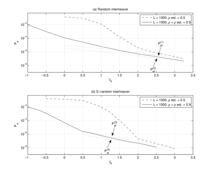
Figure 7: $P_{e}$ versus $\gamma_{b}$ for $TC$ with $L=1000$, random interleaving (a) and S-random interleaving (b): comparisons between no a-apriori ($\rho=0.5$) and a-priori with $\rho=\rho$ est. $=0.9$.

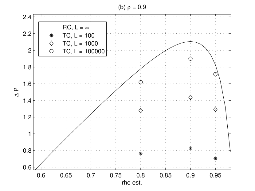
Figure 8: $\Delta P$ versus the estimated $\rho$ (i.e., ${\tilde{\rho}}$ is in the abscissa) for ${P}_{e,r}=0.00001$: comparisons between random codes (RC) analysis with $L=\infty$ (39) and turbo codes ($TC$) with different $L$, for: (a) $\rho=0.7$, (b) $\rho=0.9$

where $A$ is defined in (19).
As it is well known, performance of turbo codes can be improved by a more accurate design of the interleaver [27]. As an example, S-random interleavers [25] allow to avoid short cycle events, i.e., two bits which are close to each other both before and after interleaving. For comparison purposes, we then consider a specific interleaver derived by applying the S-random algorithm.
Computer simulations of a two-code turbo code system with both random and S-random interleavers have then been carried out. The constituent codes are $r=1/2$ recursive convolutional codes with constraint length $K=4$, $G^{(2)}(D)=D^{3}+D^{2}+1$, $H(D)=D^{3}+D+1$, and $G^{(1)}(D)=H(D)$, (systematic code). The overall rate of the turbo code is $r=1/3$ which is increased to $r=1/2$ via classical puncturing technique which enables to select the coded bits alternatively from the two encoders. The algorithm used by the two convolutional decoders at the receiver is based on the MAP BCJR scheme [28], which allows the inclusion of API in the form of LLRs of the input data.
Fig. 7 show the BER versus $\gamma_{b}$ for the turbo codes ($TC$) introduced above. The frame size $k$ of the information sequence (i.e., the interleaving size) is set to $k=1000$ bits and the maximum number of iterations of turbo decoding is set to 10. Performance of random (7 (a)), and S-random (7 (b)) interleavers are shown for the case of no API, i.e., $\rho=0.5$, and API with $\rho=0.9$ and perfect estimation, i.e., $\rho=\tilde{\rho}$. Theoretical curves for the random interleaving evaluated according to (40) and (41) are also shown. Note that for the considered code, $K_{1}=2/1000=0.002$. As far as $d_{2,t}$ is concerned, on account of puncturing we get $d_{2,t}=d_{2}$. The distance $d_{2}$ can be easily computed by means of the modified state diagram [22]. In particular, for the considered constituent codes we have $d_{2}=8$, which yields $d_{2,t}=8$. Eventually, we also show the theoretical curves for the S-random case. In this case a performance analysis in the error floor region can be provided by following the WSE method proposed in [29], where an union bound of the bit error probability is calculated as the partial sum of the dominant terms (corresponding to small code weights). Of course, we can also straightforwardly derive the bit error probability in presence of API by multiplying each term of the upper bound’s partial sum by $A^{w}$, $w$ being the information weight of this term. Theoretical curves for the S-random case are denoted in Fig. 7 by $P_{ef}^{(3)}$, for the $\tilde{\rho}=0.5$ case, and $P_{ef}^{(4)}$, for the $\tilde{\rho}=\rho=0.9$ case.
Several comments can be drawn by the curves shown in Fig. 7. First of all note that, as expected, S-random interleaver allows to achieve performance better than random interleaver. Moreover, for $BER\geq 10^{-5}$ the considered turbo codes allow to exploit API much better than convolutional codes considered in the previous Section. As an example, if we consider $P_{e,r}=10^{-4}$ we observe that the performance gain due to API is higher than $1.6$ dB for S-random interleaver and slightly lower than $1.5$ dB for random interleaver . Similar gains are still achieved for $P_{e,r}=10^{-5}$. This result is due to the fact that error events which mainly occur for such medium BER values are characterized by high $w$ values. Instead, as expected, in the error floor region the curves for $\rho=0.5$ and $\rho=\tilde{\rho}=0.9$ get closer since in this case the performance behavior is determined by low $w$ error events. It is also worth noting that the error floor fittings are very close to simulation results, thus confirming the validity of the proposed analysis.
Results in Fig. 7 suggest that an accurate design of the interleaver in turbo codes may help the decoder to exploit better the API (if there is any). In particular, since the constituent codes of turbo codes are convolutional codes, the possibility of avoiding small $w$ codewords is fully demanded to the possibility of the interleaver to break small weight input data sequences. Hence, even if the design of optimal interleavers in presence of API is out of the scope of this work, we can conclude that good interleaver for the classical case (no API) are good also for the case of API at the receiver.
A question which arises from previous comments is wether turbo codes allow to approach the performance gain $\Delta P$ which has been derived in the previous Section for infinite length random codes. Of course the performance gain depends in general on the target BER $P_{e,r}$ that can be accepted. If we consider $P_{e,r}=10^{-5}$ we see from Fig. 7 that such a BER is quite close to the error floor region. To increase the $\Delta P$ for such a BER is then necessary to lower the error floor region, i.e., to decrease the probability of the occurrence of low $w$ error events. As it is well known from the literature [26] this can be easily obtained by increasing the frame size $k$. Hence we have run computer simulations for different $k$ and for the S-random interleaver. Results are summarized in Fig. 8 where $\Delta P$ versus ${\tilde{\rho}}$ for ${P}_{e,r}=10^{-5}$ is shown for $\rho=0.7$ (Fig. 8 (a)), $\rho=0.9$ (Fig. 8 (b)) and for different $k$ values, namely $k=100$, $k=1000$, and $k=100000$. For comparison purposes, we also show $\Delta P$ of random codes ($RC$) with $k=\infty$ obtained through equation (39). Note that as $k$ increases up to $100000$, the performance gain due to API of $TC$s approach the theoretical gain of infinite length $RC$s. Of course this is true for ${P}_{e,r}=10^{-5}$ while, for the considerations drawn before, it could not be true anymore for a lower BER target. It is also worth noting that the theoretical analysis for $RC$s gives an accurate bound of the allowable gains that can be obtained by exploiting API at the receiver even in presence of estimation errors.

V Case study: transmission of correlated signals observed at different nodes

As discussed in the Introduction, the transmission of correlated signals observed at different nodes to one or more collectors has become a topical problem in the recent years, mainly because of the quick diffusion of Wireless Sensor Networks (WSNs). We consider in this Section a simple scenario where two independent nodes have to transmit correlated sensed data to a collector node. Such data, referred to as $x_{i}$ and $y_{i}$, are taken to be i.i.d. correlated binary randon variables with $P_{r}\left\{x_{i}=1/0\right\}=P_{r}\left\{y_{i}=1/0\right\}=0.5$ and correlation $\rho=P_{r}\left\{x_{i}=y_{i}\right\}>0.5$. We consider a very simple Joint Source Channel Decoding (JSCD) technique where no source encoding is performed (i.e., no compression) but the two transmitters send their data over independent AWGN channels using the $r=1/2$ punctured turbo code described in the previous Section. The independence of the noise terms in different links is due to the fact that the nodes are assumed to transmit over orthogonal multiple access channels (e.g., using frequency division multiple access). At the receiver two independent decoders performs an iterative decoding scheme where, at iteration $m$, the first decoder gives an estimation $x^{(m)}_{i}$ of $x_{i}$ and the second decoder gives an estimation $y^{(m)}_{i}$ of $y_{i}$. To achieve this goal, the first/second decoder observes the signal coming from the first/second channel and performs turbo decoding taking $y^{(m-1)}_{i}$/$x^{(m-1)}_{i}$ as API. The correlation estimation $\tilde{\rho}$ is evaluated at iteration $m$ as:

$$\begin{array}[]{cl}\tilde{\rho}^{(m)}=\frac{1-\sum\limits_{i=0}^{k-1}x^{(m-1)}_{i}\oplus y^{(m-1)}_{i}}{k}\end{array}$$ (42)

Note that at first iteration ($m=0$) neither the correlation nor the API are available at the two decoders and hence the first decoding step is performed by setting $\tilde{\rho}^{(0)}=0.5$. In this way the decoder does not need any knowledge about the correlation between the transmitter data. On the other hand, the theoretical analysis provided in the previous Sections show that the decoder performance is not very sensitive to estimation error (see Fig. 8). Hence, we expect that the decoder works well even in presence of imperfect correlation estimation and that it iteratively converges to achieve an almost perfect correlation estimation.
We compare the proposed JSCD technique with the ideal separation-based strategy where the to-be-transmitted data are firstly compressed at the minimum achievable compression rate and then transmitted into the channel by means of turbo channel coding. Note that in this case the two transmitters must implement distributed source coding (DSC), and thus they must have a perfect correlation estimation (supposedly, correlation is still estimated at the receiver and then it is sent to the transmitters by means of a feedback channel). On the other hand, even in presence of perfect correlation estimation, the problem of designing good practical source codes for correlated sources is still open. Hence, this second scheme can be considered as an ideal transmission scheme. In the DSC case, the two sources $x_{i}$ and $y_{i}$ are independent (on account of compression) and, hence, decoding is performed without any API. To provide a fair comparison with the proposed JSCD technique we assume that in the separation case the rate of the channel encoder is lower, so that the global transmission rates is the same for the two cases. To elaborate, let assume a correlation $\rho=0.939$ between the two sources. In this case the joint entropy of the two information signals is $H({\mathbf{x}},{\mathbf{y}})$ = $H({\mathbf{x}})$ + $H({\mathbf{x}}|{\mathbf{y}})$ = $1-\rho\times log_{2}(\rho)-(1-\rho)\times log_{2}(1-\rho)$ = $1.33$. This means that the two transmitters may achieve a compression rate of $r_{c}=1.33/2=2/3$ . Hence, in order to achieve the same rate $r=1/2$ as the JSCD case, in the separation case the channel coding rate may be set to $1/3$. This can be achieved by using the unpunctured version of the turbo code described in the previous Section. Moreover, we consider the same signal-to-noise ratio $SNR=2r\gamma_{b}$ for JSCD and DSC, so that the two schemes are compared for the same overall transmitted rate and the same same total transmitted energy. Note that, since the channel rate in the DSC case is 3/2 times lower than in the JSCD case, the $\gamma_{b}$ value is $3/2$ times higher (i.e, 1.76 dB higher). In other terms, we compare the rate $r=1/2$ JSCD scheme with a given $\gamma_{b}=\gamma$ dB with the rate $r=1/3$ DSC scheme with $\gamma_{b}=\gamma+1.76$ dB.
Fig. 9 show a BER comparisons between the JSCD and DSC scenarios described above. In particular, in Fig. 9 (a) we consider an AWGN channel model where the two channels are characterized by the same $SNR$. In Fig. 9 (b) we instead consider a block Rayleigh fading channel model where $SNR$ is exponentially distributed with the same average $E(SNR)$ in the two channels. As far as the turbo code is of concern, the frame size $k$ of the interleaver is set to $k=1000$ bits and the maximum number of iterations is set to 10.
Note that in the AWGN case, for a target $P_{e}=0.00001$, the performance of the proposed JSDC scheme is only 0.2 dB worse than the ideal DSC scheme. This assesses the validity of the proposed iterative JSCD scheme based on turbo coding. The most interesting and, dare we say, surprising results is derived in the Rayleigh case, where the JSDC decoding scheme clearly outperform DSC with a gain of more then 7 dB for $P_{e}=0.001$. The rationale for this result is that in presence of an unbalanced signal quality from the two transmitters (e.g., independent fading), leaving a correlation between the two information signals can be helpful since the better quality received signal can be used as side information for detecting the other signal. In other words, the proposed JSCD scheme allows to get a diversity gain $K$ which is not obtainable by the DSC scheme. The diversity gain can be measured as the gradient of the BER curve, which yields $K=1$ in the DSC case and $K\cong 1.32$ in the JSCD case. Such a diversity gain is due to the inherent correlation between information signals and, hence, can be exploited at the receiver without implementing any kind of cooperation between the transmitters.

VI Conclusions

We have derived a novel analysis for evaluating decoding performance in presence of a-priori information with imperfect correlation estimation. According to this analysis, it is shown that the performance depends not only on the codewords’ weight, as in traditional decoding, but also on the information data weight. We have then validated the proposed analysis in three different scenarios: convolutional codes, random codes and turbo codes. In particular, turbo codes have been shown to approach the performance of infinite length random codes. Moreover, we have proposed an effective joint source-channel decoding scheme in a wireless sensors network scenario where two nodes detect correlated sources and deliver them to a central collector. Experimental results show the the proposed scheme allows to approach the ideal Slepian-Wolf scheme in AWGN channel, and to clearly outperform it over fading channels on account of a diversity gain which can be achieved without implementing any kind of cooperation between the transmitters.

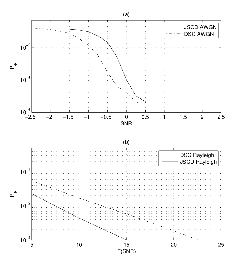
Figure 9: BER comparison between JSCD and DSC for : (a) AWGN (b) Rayleigh fading

References

- [1] J. Hagenauer, ”Source-Controlled Channel Decoding,” Communications, IEEE Transaction on, Vol.43, No. 9, Sep. 1995.
- [2] M. Park and D. J. Miller, ” Joint source-channel decoding for variable length encoded data by exact and approximate MAP sequence estimation,” Communications, IEEE Transaction on, Vol.48, No. 1, pp. 1-6, Jan. 2000.
- [3] C. Lamy and O. Pothier, ”Reduced complexity maximum a posteriori decoding of variable-length codes,” Proc. IEEE GLOBECOM, San Antonio, TX vol. 2, pp. 1410-1413, Nov. 2001.
- [4] M. Jeanne, J. C. Carlach, P. Siohan, ”Joint source-channel decoding of variable-length codes for convolutional codes and turbo codes,” Communications, IEEE Transaction on, Vol. 53, No. 1, Jan. 2005.
- [5] Xiaobei Liu, Soo Ngee Koh, and Tee Hiang Cheng, ”Improved Bit-Based Joint Source-Channel Decoding of Variable Length Codes,” IEEE Communications Letters, Vol. 11, No. 6, June 2007.
- [6] P. M. Crespo, E. Loyo, J. Del Ser and C. J. Mitchell, ”Source Controlled Modulation Scheme for Sources with Memory,” Proc. IEEE International Conference on Communication (ICC), Glasgow, Scotland, 24-28 June, 2007.
- [7] Guang-Chong Zhu, Fady Alajaji, ”Joint Source-Channel Turbo Coding for Binary Markov Sources,” IEEE TRANSACTIONS ON WIRELESS COMMUNICATIONS, Vol. 5, No. 5, May 2006.
- [8] Lingling Pu, Zhenyu Wu, Ali Bilgin, Michael W. Marcellin, Ali Bilgin, ”LDPC-Based Iterative Joint Source-Channel Decoding for JPEG2000,” IEEE TRANSACTIONS ON IMAGE PROCESSING, Vol. 16, No. 2, Feb. 2007.
- [9] I. F. Akyildiz, W. Su, Y. Sankasubramaniam, and E. Cayirci ”Wireless Sensor Networks: A Survey,” Computer Networks Vol. 38, pp. 393-422, 2002
- [10] J. Barros and S. Servetto ”On the capacity of the reachback channel in wireless sensor networks,” IEEE Workshop on Multimedia Signal Processing, pp. 408-411, 2002.
- [11] P. Gupta and P. Kumar ”The capacity of wireless networks,” IEEE Transactions on Information Theory 46, March 2000
- [12] H. E. Gamal ”On the scaling laws of dense wireless sensor networks,” IEEE Transactions on Information Theory April 2003
- [13] A. Aaron and B. Girod ”Compression with side information using turbo codes,” Proc. IEEE Data Compression Conference Snowbird, Utah, Apr. 2002
- [14] J. Bajcsy and P. Mitran ”Coding for the Slepian-Wolf problem with turbo codes,” Proc. IEEE Proc. Global Telecommu. Conf. Nov. 2001
- [15] I. Deslauriers and J. Bajcsy ”Serial Turbo Coding for Data Compression and the Slepian-Wolf Problem,” Proc. Information Theory Workshop Mar. 2003
- [16] Z. Xiong, A. D. Liveris, and S. Cheng ”Distributed source coding for sensor networks,” IEEE Signal Process. Mag., Sep. 2004
- [17] J. Garcia-Frias and Y. Zhao ”Compression of correlated binary sources using turbo codes,” IEEE. Communications Letters vol. 5, no. 10, pp. 417-419, October 2001
- [18] Y. Zhao and J. Garcia-Frias ”Joint Estimation and Compression of Correlated Nonbinary Sources Using Punctured Turbo Codes,” IEEE. Transactions on Communications vol. 53, no. 3, pp. 385-390, March 2005
- [19] J. Garcia-Frias, Y. Zhao and W. Zhong ”Turbo-like codes for Transmission of Correlated Sources over Noisy Channels,” IEEE. Signal Processing Magazine pp. 58-66, September 2007
- [20] F. Daneshgaran, M. Laddomada, M. Mondin, ”Iterative Joint Channel Decoding of Correlated Sources Employing Serially Concatenated Convolutional Codes,” Information Theory, IEEE Transaction on, Aug. 2005 Volume: 51, Issue: 7
- [21] J. Maramatsu, T. Uyematsu, T. Wadayama, ”Low-density Parity-Check Matrices for Coding of Correlated Sources,” Information Theory, IEEE Transaction on, October 2005 Volume: 51, Issue: 10
- [22] B Sklar, ”Digital Communications: Fundamentals and Applications,” New Jersey, Prentice Hall, 2001
- [23] John G. Proakis ”Digital Communications,” Singapore: Mc Graw-Hill, 1995.
- [24] Holger Karl, Andreas Willig ”Protocols and Architectures for Wireless Sensor Networks,” Chichester, England: John Wiley and Sons, 2006.
- [25] D. Divsalar, S. Dolinar, R. J. McEliece, and F. Pollara ”Performance Analysys of Turbo Codes,” IEEE MIlcom Vol. 1, pp. 91-96, Nov. 1995.
- [26] S. Benedetto and G. Montorsi ”Unveiling turbo codes: some results on parallel concatenated coding schemes,” IEEE. Transactions on Information Theory vol. 42, pp. 409-428, Mar. 1996.
- [27] H. R. Sadjadpour, N. J. A. Sloane, M. Salehi, and G. Nebe ”Interleaver Design for Turbo Codes,” IEEE JOURNAL ON SELECTED AREAS IN COMMUNICATIONS, Vol. 19, No. 5, May 2001.
- [28] L. Bahl, J. Cocke, F. Jelinek, and J. Raviv, ”Optimum decoding of linear codes for minimizing symbol error rate,” IEEE Trans. Inform. Theory, vol. IT-20, pp. 284 287, Mar. 1974.
- [29] P. C. Yeh, O. Yilmaz, W. Stark ”On the Error Floor Analysis of Turbo Code: Weight Spectrum Estimation (WSE) Scheme,” ISIT 2003, Yokohama, Japan, June 29 - July 4, 2003.