Pre-asymptotic corrections to fractional diffusion equations

Abstract

The motion of contaminant particles through complex environments such as fractured rocks or porous sediments is often characterized by anomalous diffusion: the spread of the transported quantity is found to grow sublinearly in time due to the presence of obstacles which hinder particle migration. The asymptotic behavior of these systems is usually well described by fractional diffusion, which provides an elegant and unified framework for modeling anomalous transport. We show that pre-asymptotic corrections to fractional diffusion might become relevant, depending on the microscopic dynamics of the particles. To incorporate these effects, we derive a modified transport equation and validate its effectiveness by a Monte Carlo simulation.

I Introduction

A diffusion process is called anomalous when the variance of the transported quantity, $\left\langle x^{2}(t)\right\rangle$, grows in time as $t^{\alpha}$, with $\alpha$ larger (superdiffusion) or smaller (subdiffusion) than one. A general approach to the analysis of stochastic transport is based on the continuous time random walk (CTRW), a probabilistic model where the motion of a walker in a medium is interpreted as a series of jumps of random lengths, separated by random waiting times beyondbm ; klafter1 ; klafter2 ; weiss . The theory of CTRW with power-law probability distribution functions (pdf’s) for the waiting times was first introduced in physics in the late 1960s to describe anomalous diffusion of charge carriers in amorphous semiconductors scher_lax1 ; scher_lax2 ; scher ; montroll . It was later applied with success to a broad spectrum of physical systems (see, for example, Refs. klafter1 and klafter2 for a review).

As a paradigmatic example of anomalous diffusion we consider here the case of contaminant transport through heterogeneous materials, such as porous sediments or fractured rocks. In this system the microscopic dynamics of each particle is assumed to be hindered by obstacles, dead ends, trapping events due to the interaction with the surrounding environment or abrupt changes in the flow field. The macroscopic effect is that the spread of the migrating particles plume grows sublinearly in time, thus resulting in subdiffusion cortis_gallo ; cortis_berkowitz ; berkowitz_klafter ; berkowitz_kosakowski ; berkowitz_scher ; berkowitz_scher2 ; dentz_cortis ; levy_berkowitz ; margolin . These assumptions are substantially corroborated by many experimental observations kimmich ; klemm1 ; berkowitz_klafter ; berkowitz_kosakowski ; cortis_berkowitz .

In general, the CTRW equations do not allow for closed-form analytical solutions. However, if suitable first-order approximations are introduced, a fractional diffusion equation can be formally derived from CTRW and analytical solutions can be obtained: in this respect, the fractional diffusion equation represents an asymptotic subset of CTRW beyondbm ; klafter1 ; klafter2 ; barkai ; schneider ; sokolov .

A complementary approach to the modeling of stochastic transport is provided by Monte Carlo simulation, a particle tracking method which allows the fate of each walker to be followed by sampling the jump lengths and the waiting times from a suitable distribution. Monte Carlo simulation has been widely adopted as a natural tool to obtain reliable and accurate estimates of the CTRW solutions dentz_cortis .

In this paper, we explore the range of validity of the asymptotic fractional diffusion equation. This topic has been previously examined e.g. in Refs. barkai1 and barkai2 . With the help of Monte Carlo simulations, building on the discussion in Refs. margolin and marseguerra_zoia1 , we show that pre-asymptotic corrections to the fractional diffusion equations play a significant role, depending on the microscopic dynamics of the particles . Neglect of these corrections would lead to gross errors in the estimation of model parameters from measured data. To overcome this problem, we derive a modified equation which incorporates these effects.

The paper is organized as follows. In Sec. II we review the CTRW model and the asymptotic fractional diffusion equation. In Sec. III we show that for a given range of a critical parameter the fractional diffusion equation might not properly characterize the actual spread of the transported quantity as derived from CTRW (through a Monte Carlo estimate). We discuss how to modify the fractional diffusion model so to include the contribution of pre-asymptotic corrections and validate the proposed results by comparing them to Monte Carlo simulations. Conclusions are discussed in Sec. IV.

II From CTRW to fractional diffusion

We briefly review here the main assumptions of the CTRW model. Consider a walker whose stochastic trajectory in a medium is modeled as a series of random jumps separated by random waiting times, during which the walker stays in the previously reached position. The associated pdf $P(x,t)$ represents the probability density of the walker being at $x$ at time $t$ and is usually called the propagator of the process. For contaminant transport, $P(x,t)$ represents the normalized particle concentration. The properties of the propagator depend on the jump lengths pdf $\lambda(x)$ and the waiting times pdf $w(t)$. Once these distributions are assigned, it is possible to derive a probability equation for $P(x,t)$, the master equation of the CTRW model klafter1 ; weiss ; scher ; montroll It can be shown klafter1 that the master equation in $\{x,t\}$ space can be recast into a simple algebraic relation for the Fourier and Laplace transformed propagator $P(k,u)={\cal L}\left\{{\cal F}\{P(x,t)\}\right\}$

$$P(k,u)=\frac{1-w(u)}{u}\frac{1}{1-\lambda(k)w(u)},$$ (1)

with the walkers starting at $x=0$ at time $t=0$.

Within the CTRW scheme the long waiting times which characterize the trajectory of a contaminant particle moving through heterogeneous materials are taken into account by assuming that $w(t)$ has a power-law tail $w(t)\sim t^{-1-\alpha}$, $\alpha<1$, when $t\rightarrow+\infty$. Therefore, $w(t)$ lacks a characteristic time scale (the average of the distribution is infinite) and anomalously long waiting times have a non-negligible probability of being sampled. In the following we will assume a Pareto pdf of the form

$$w(t)=\alpha\tau^{\alpha}t^{-1-\alpha},\qquad(t\geq\tau)$$ (2)

where $\tau$ is a time constant. This specific form for $w(t)$ has been chosen so that Monte Carlo sampling by inverse transform is straightforward: it can be shown that the short time behavior of the pdf is of minor importance and only the tail matters in determining the properties of $w(t)$ feller . The jump length pdf $\lambda(x)$ is usually assumed to be a Gaussian distribution, so that the jumps have a typical scale (say the standard deviation of the distribution) and extreme events, that is, jumps whose length are much larger than the standard deviation, are very improbable.

In general, no analytical solution is known for Eq. (1), because the required inverse transforms are usually not trivial. However, exact results can be obtained for $P(x,t)$ sufficiently far from the origin, in the diffusion limit $|x|\to+\infty,t\to+\infty$, that is, $k\to 0,u\to 0$ (see, for example, Ref. barkai for a detailed discussion).

If $w(u)={\cal L}\left\{w(t)\right\}$ is expanded in the long time limit $u\tau\ll 1$ and truncated to the first non-constant term in $u$, we find $w(u)\simeq 1-c_{\alpha}(u\tau)^{\alpha}$, where $c_{\alpha}=\Gamma(1-\alpha)$. More generally, it can be shown that any pdf of the kind $w(t)\sim t^{-1-\alpha}$ would lead to the same expansion $w(u)$ in the transformed space; the specific value of the constant $c_{\alpha}$ depends on the details of the function feller ; klafter1 . In contrast, if $\lambda(x)$ is a Gaussian with mean $\mu=0$ and variance $2\sigma^{2}$, then $\lambda(k)={\cal F}\left\{\lambda(x)\right\}$ becomes $\lambda(k)\simeq 1-k^{2}\sigma^{2}$ in the diffusion limit $k\sigma\ll 1$. Any jump pdf with finite variance would asymptotically lead to the same result klafter1 .

We now introduce the Riemann-Liouville fractional derivative operator podlubny ; miller_ross ; kilbas $\partial^{1-\alpha}_{0,t}$, which is defined by its action on a sufficiently well behaved function $f$:

$$\partial^{1-\alpha}_{0,t}f(t)=\frac{d}{dt}\partial^{-\alpha}_{0,t}=\frac{1}{\Gamma(\alpha)}\frac{d}{dt}\int_{0}^{t}\frac{f(t^{\prime})}{(t-t^{\prime})^{1-\alpha}}dt^{\prime}.$$ (3)

The Riemann-Liouville operator is an integro-differential operator involving a convolution integral with a power-law kernel. In particular, the operator $\partial^{-\alpha}_{0,t}$ may be thought as a generalization of the usual multiple integral of integer order. From its definition, $\partial^{-\alpha}_{0,t}$ has a very simple representation in $\cal L$-space: ${\cal L}\left\{\partial^{-\alpha}_{0,t}f(t)\right\}=u^{-\alpha}f(u)$, $\forall\alpha>0$ podlubny ; miller_ross ; kilbas .

If we substitute $w(u)$ and $\lambda(k)$ in Eq. (1) and make use of the definition (3), we can formally write the propagator (1) in the $\left\{x,t\right\}$ space:

$$\frac{\partial}{\partial t}P(x,t)=D_{\alpha}\partial^{1-\alpha}_{0,t}\frac{\partial^{2}}{\partial x^{2}}P(x,t),$$ (4)

where $D_{\alpha}=\sigma^{2}/c_{\alpha}\tau^{\alpha}$ may be thought as a generalized diffusion coefficient klafter1 . Equation (4), which is called the fractional diffusion equation due to its fractional derivative, is a generalization of the classical Fickian diffusion equation and describes the asymptotic behavior of a plume of subdiffusive particles in the absence of advection. A more general fractional differential equation was derived from CTRW in Refs. afanasiev and zavslasky_chaos . The power-law kernel in $\partial^{1-\alpha}_{0,t}$ decays slowly and macroscopically represents the long-range correlations induced by the obstacles that the particles encounter zavslasky_chaos ; mainardi . If $\alpha>1$, the correlations decay sufficiently quickly so that normal diffusion is recovered klafter1 .

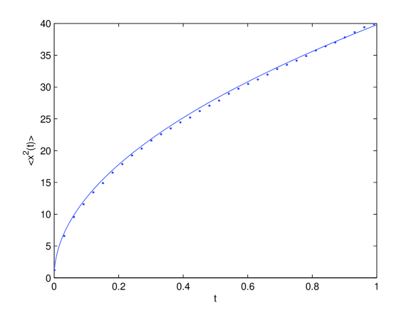
Figure 1: Comparison between the analytical result (Eq. (5), solid line) and the Monte Carlo variance (dots) as a function of time for $\alpha=0.5$. The agreement is remarkable.

In the context of contaminant transport it is of utmost importance to determine the evolution of the plume spread as a function of time. This physical quantity corresponds to the variance of the propagator. From the fractional diffusion equation it may be expressed in closed form as:

$$\left\langle x^{2}(t)\right\rangle\equiv-\lim_{k\rightarrow 0}\frac{\partial^{2}}{\partial k^{2}}{\cal L}^{-1}\left\{P(k,u)\right\}=\frac{2D_{\alpha}}{\Gamma(1+\alpha)}t^{\alpha}.$$ (5)

Because $\alpha<1$, the plume migration is subdiffusive, as expected.

III Higher-order corrections to fractional diffusion

In principle, Eq. (5) provides a reliable estimate of the actual contaminant spread when the diffusion limit is attained, that is, $k\sigma\ll 1$ and $u\tau\ll 1$, so that the fractional diffusion equation is a good asymptotic expansion of CTRW. To assess this statement, we compare the analytical variance (5) with Monte Carlo simulation results for two values of $\alpha$. Monte Carlo estimates, which are obtained by simulating the microscopic dynamics of the particles, will be assumed as a reference solution of CTRW. In the first example, $10^{5}$ particles were followed up to a time $t_{\max}=1$, with the simulation parameters $\alpha=0.5$, $\sigma=0.5$, and $\tau=10^{-4}$ (see Fig. 1). In this case the fractional diffusion prediction (5) agrees perfectly with the Monte Carlo simulation.

Next we let $\alpha=0.8$, with $\sigma=0.5$, $\tau=10^{-4}$, and $t_{\max}=1$ (see Fig. 2). In this case the fractional diffusion prediction (5) underestimates the actual Monte Carlo spread, so that fractional diffusion cannot be considered a good approximation of CTRW. The error introduced by the fractional diffusion prediction is far beyond the fluctuations due to the finite Monte Carlo statistics. We remark that in both cases the explored time scales are such that $\tau\ll t_{\max}$, thus ensuring that the diffusion limit has been attained.

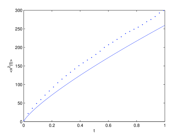
Figure 2: Comparison between the analytical (Eq. (5), solid line) and Monte Carlo results (dots) as a function of time for $\alpha=0.8$. There is a clear disagreement.

What is the origin of the discrepancies shown in Fig. 2? Straightforward but tedious calculations show that the expansion of $w(u)$ to second order in $u$ yields:

$$w(u)=1-c_{\alpha}(u\tau)^{\alpha}-c_{1}(u\tau)+o(u^{2}),$$ (6)

where $c_{1}=\alpha/(\alpha-1)$. Therefore, when the exponent $\alpha$ is small, the linear term in $u$ in Eq. (6) is expected to play no significant role in the limit $u\tau\ll 1$, thus justifying the accuracy of the fractional diffusion equation predictions. In contrast, if $\alpha\rightarrow 1$, the two terms in the expansion (6) become comparable and the effects of the linear contribution will no longer be negligible margolin ; marseguerra_zoia1 . More precisely, when $\alpha<1$ the contribution of $c_{1}(u\tau)$ will always be subdominant with respect to $c_{\alpha}(u\tau)^{\alpha}$ (for $u\to 0$), so that after a sufficiently long time ($t\gg\tau$) we always recover the fractional diffusion equation as the correct asymptotic limit of CTRW. In this respect the term $c_{1}(u\tau)$ introduces pre-asymptotic corrections to the behavior of the subdiffusive particles. However, the values of $\alpha$ and $\tau$ are usually imposed by experiment and inherently linked to the choice of $w(t)$, that is, to the microscopic dynamics of the particles. It is therefore interesting to systematically explore the behavior of the CTRW and fractional diffusion solutions for intermediate time scales where the diffusion limit $u\tau\ll 1$ holds but the truncation of (6) to the first non-constant term might not be appropriate, depending on the value of $\alpha$.

To quantitatively assess the relevance of the contribution $c_{1}(u\tau)$ in the expansion of $w(u)$, we substitute Eq. (6) into the propagator (1), to obtain:

$$uP(k,u)-1=-\frac{\sigma^{2}k^{2}}{c_{\alpha}\tau^{\alpha}u^{\alpha-1}+c_{1}\tau}P(k,u).$$ (7)

By making use of the formal properties of the Riemann-Liouville operators, Eq. (7) may be finally recast into a modified fractional derivative equation

$$\frac{\partial}{\partial t}P(x,t)=D_{\alpha}\partial^{1-\alpha}_{0,t}\frac{\partial^{2}}{\partial x^{2}}P(x,t)+q_{\alpha,1}\partial^{1-\alpha}_{0,t}\left\{\frac{\partial}{\partial t}P(x,t)\right\},$$ (8)

where $q_{\alpha,1}=c_{1}\tau/c_{\alpha}\tau^{\alpha}$ . If $\alpha$ is sufficiently small, we can expand

$$\frac{1}{c_{\alpha}\tau^{\alpha}u^{\alpha-1}+c_{1}\tau}=\frac{u^{1-\alpha}}{c_{\alpha}\tau^{\alpha}}\left(\frac{1}{1+q_{\alpha,1}u^{1-\alpha}}\right)\simeq\frac{u^{1-\alpha}}{c_{\alpha}\tau^{\alpha}}\left(1-q_{\alpha,1}u^{1-\alpha}\right)\simeq\frac{u^{1-\alpha}}{c_{\alpha}\tau^{\alpha}}+o(u^{2-2\alpha}),$$ (9)

so that we recover the standard fractional diffusion equation. If instead $\alpha$ is of the order of unity, the two terms $c_{\alpha}(u\tau)^{\alpha}$ and $c_{1}(u\tau)$ (which are mirrored in the $D_{\alpha}\partial^{1-\alpha}_{0,t}$ and $q_{\alpha,1}\partial^{1-\alpha}_{0,t}\frac{\partial}{\partial t}$ operators, respectively) are in competition, and their specific contributions to the overall functional form of the propagator $P(x,t)$ cannot be neglected. We argue that Eq. (8), which is the central result of our work, also provides a suitable description of the particle dynamics for pre-asymptotic time scales. To support this argument we compute the spread associated to Eq. (8). By definition,

$$\left\langle x^{2}(t)\right\rangle={\cal L}^{-1}\left\{\frac{2\sigma^{2}}{u^{2}}\frac{1}{c_{\alpha}\tau^{\alpha}u^{\alpha-1}+c_{1}\tau}\right\}.$$ (10)

The inverse $\cal L$ transform appearing in Eq. (10) can be computed numerically dehoog ; hollenbeck . The curves thus obtained are again compared with Monte Carlo simulation. Figure 3 clearly shows that the modified Eq. (8) provides a reliable estimate of the system evolution even at pre-asymptotic time scales.

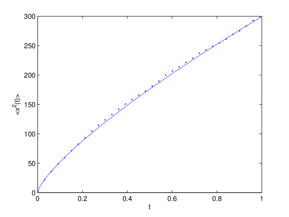
Figure 3: Comparison between the variance (10) as obtained by numerical inversion (solid line) and Monte Carlo simulations (dots) for $\alpha=0.8$. The two curves are in excellent agreement.

IV Conclusions

The fractional diffusion equation arises as an asymptotic approximation to an exact master equation and suffers from some limitations barkai . As an example, although anomalous diffusion is often experimentally found to be a transient phase, which after a suitable time scale generally relaxes to Fickian diffusion, the fractional diffusion equation cannot take into account for this transition because the anomalous behavior is assumed to hold even at infinite time cortis_gallo ; dentz_cortis ; klafter1 ; klafter2 ; schneider . Moreover, the CTRW formulation in terms of a generalized Fokker-Planck equation with a memory kernel recently proposed e.g. in cortis_gallo can take into account more general expressions for $w(u)$ (as compared to to those allowed by the fractional derivative approach), as well as boundary and initial conditions in multiple dimensions. In this respect, the CTRW formalism, thanks to its greater flexibility, can capture and quantify more general tranport instances, as shown e.g. in cortis_ex1 ; cortis_ex2 .

It must be also emphasized that not all anomalous diffusion phenomena can be represented in a fractional derivative formalism, since anomalous diffusion is usually context-dependent many specific realizations do not fall within this framework (even though enlarged so to include pre-asymptotic corrections). This is the case, for instance, of the diffusion problems studied by cortis_knudby , where slower than Fickian, but faster than algebraic decays are found, or by zoia_kardar , where anomalous transport in a fracture network gives rise to a scaling which is at variance with the power-law predicted by the fractional derivative framework.

Nonetheless, a relevant feature of the fractional diffusion equation (in spite of its limitations) is that the fractional derivative formulation may easily include external fields in a simple manner and is naturally suitable for solving boundary value problems metzler_klafter ; zoia . In this respect, the fractional diffusion equation has been recently shown to act as a unifying framework for the quantitative description of different physical phenomena where anomalous diffusion plays a significant role klafter1 ; klafter2 . Moreover, many standard mathematical techniques for solving partial differential equations are readily applicable to the fractional diffusion equation.

In the context of particle transport in heterogeneous materials the fractional diffusion formulation may be used to analyze the evolution of the contaminant plume spread in time. Comparing the model prediction with measured experimental data could then lead to an estimate of the exponent $\alpha$ characterizing the system. It is therefore important to quantify the limit of validity of the fractional diffusion asymptotic subset. In this paper we have shown that, if $\alpha\to 1$, the pre-asymptotic corrections to fractional diffusion might significantly affect the model predictions. Their neglect would induce gross errors in the model which would distort the estimate of $\alpha$. To overcome this problem, we have derived a modified transport equation involving fractional derivatives: we have shown that the particle spread predicted by this model is in excellent agreement with Monte Carlo simulation also at the pre-asymptotic time scales. This modified equation might be suitable to explore the subdiffusive dynamics of physical systems close to the limit $\alpha\to 1$.

Finally, we remark that analogous pre-asymptotic corrections would come into play also in the case of diffusive dynamics ($\alpha>1$), if we were to adopt a power-law decaying distribution for the waiting times. These corrections would have a significant role close to the limit $\alpha\to 1$ and their origin is in the nature of the functional form of $w(t)$. Only, the role of the two contributions would be the opposite with respect to the case examined in this work: the dominant contribution would come from the term in $u$, the term in $u^{\alpha}$ being subdominant for $u\to 0$, as expected. As a particular case, it is also possible to choose the (arbitrary) waiting time distribution so that the coefficient $c_{1}$ is identically zero: a widely adopted choice is assuming a Lévy stable law for $w(t)$, so that its Laplace transform expansion would not contain the term in $u$.

- (1) J. Klafter, M. F. Shlesinger, and G. Zumofen, “Beyond Brownian motion”, Phys. Today 49 (2), 33–39 (1996).
- (2) R. Metzler and J. Klafter, “The random walk’s guide to anomalous diffusion: A fractional dynamics approach”, Phys. Reports 339, 1–77 (2000).
- (3) R. Metzler and J. Klafter, “The restaurant at the end of the random walk: Recent developments in the description of anomalous transport by fractional dynamics”, J. Phys. A: Math. Gen. 37, R161–R208 (2004).
- (4) G. H. Weiss, Aspects and Applications of the Random Walk (North Holland, Amsterdam, 1994).
- (5) H. Scher and M. Lax, “Stochastic transport in a disordered solid. I. Theory”, Phys. Rev. B 7, 4491–4502 (1973).
- (6) H. Scher and M. Lax, “Stochastic transport in a disordered solid. II. Impurity conduction”, Phys. Rev. B 7, 4502–4519 (1973).
- (7) H. Scher and E. W. Montroll, “Anomalous transit-time dispersion in amorphous solids”, Phys. Rev. B 12, 2455–2477 (1975).
- (8) E. W. Montroll and G. H. Weiss, “Random walks on lattices. II”, J. Math. Phys. 6, 167–181 (1965).
- (9) A. Cortis, C. Gallo, H. Scher, and B. Berkowitz, “Numerical simulation of non-Fickian transport in geological formations with multiple-scale heterogeneities”, Water Resour. Res. 40, W04209-1–16 (2004).
- (10) A. Cortis, and B. Berkowitz, “Anomalous transport in ‘classical’ soil and sand columns”, Soil Sci. Soc. Am. J. 68, 1539–1548 (2004).
- (11) B. Berkowitz, J. Klafter, R. Metzler, and H. Scher, “Physical pictures of transport in heterogeneous media: Advection-dispersion, random-walk, and fractional derivative formulations”, Water Resour. Res. 38 (10), 1191–1203 (2002).
- (12) B. Berkowitz, G. Kosakowski, G. Margolin, and H. Scher, “Application of continuous time random walk theory to tracer test measurements in fractured and heterogeneous porous media”, Ground Water 39, 593–604 (2001).
- (13) B. Berkowitz and H. Scher, “The role of probabilistic approaches to transport theory in heterogeneous media”, Transp. Porous Media 42, 241–263 (2001).
- (14) B. Berkowitz and H. Scher, “Anomalous transport in random fracture networks”, Phys. Rev. Lett. 79, 4038–4041 (1997).
- (15) M. Levy and B. Berkowitz, “Measurement and analysis of non-Fickian dispersion in heterogeneous porous media”, J. Contam. Hydr. 64, 203–226 (2003).
- (16) M. Dentz, A. Cortis, H. Scher, and B. Berkowitz, “Behavior of solute transport in heterogeneous media: Transition from anomalous to normal transport”, Adv. Water Resour. 27 (2), 155–173 (2004).
- (17) G. Margolin and B. Berkowitz, “Continuous time random walks revisited: First passage time and spatial distributions”, Physica A 334 46–66 (2004)
- (18) R. Kimmich, “Strange kinetics, porous media, and NMR”, Chem. Phys. 284, 253–285 (2002).
- (19) A. Klemm, R. Kimmich, and M. Weber, “Flow through percolation clusters: NMR velocity mapping and numerical simulation study”, Phys. Rev. E 63, 041514-1-8 (2001).
- (20) E. Barkai, “Fractional Fokker-Planck equation, solution, and application”, Phys. Rev. E 63, 046118-1–17 (2001).
- (21) W. R. Schneider and W. Wyss, “Fractional diffusion and wave equations”, J. Math. Phys. 30, 134–144 (1989).
- (22) I. Sokolov, J. Klafter, and A. Blumen, “Fractional kinetics”, Phys. Today 55 (11), 48–54 (2002).
- (23) E. Barkai, “CTRW Pathways to the Fractional Diffusion Equation”, Chemical Physics 284, 13 (2002).
- (24) E. Barkai, R. Metzler, and J. Klafter, “From Continuous Time Random Walks to Fractional Fokker–Planck Equation”, Phys. Rev. E 61, 132 (2000).
- (25) M. Marseguerra and A. Zoia, “The Monte Carlo and fractional kinetics approaches to the underground anomalous subdiffusion of contaminants”, Ann. Nucl. En. 33, 223–235 (2006).
- (26) A. Zoia, A. Rosso, and M. Kardar, “Fractional Laplacian in Bounded Domains”, Phys. Rev. E 76 021116 (2007).
- (27) W. Feller, An Introduction to Probability Theory and its Applications (John Wiley & Sons, New York, 1971), Vol. I.
- (28) I. Podlubny, Fractional Differential Equations (Academic Press, London, 1999).
- (29) K. S. Miller and B. Ross, An Introduction to the Fractional Calculus and Fractional Differential Equations (John Wiley & Sons, New York, 1993).
- (30) A. A. Kilbas, H. M. Srivastava, and J. J. Trujillo, Theory and Applications of Fractional Differential Equations (Elsevier, Amsterdam, 2006).
- (31) V. V. Afanasiev, R. Z. Sagdeev, and G. M. Zaslavsky, “Chaotic jets with multifractal space-time random walk”, Chaos 1, 143–159 (1991).
- (32) G. M. Zaslavsky, “Chaos, fractional kinetics, and anomalous transport”, Phys. Reports 371, 461–580 (2002).
- (33) F. Mainardi, M. Raberto, R. Gorenflo, and E. Scalas, “Fractional calculus and continuous-time finance II: The waiting-time distribution”, Physica A 287, 468–481 (2000).
- (34) F. R. de Hoog, J. H. Knight, and A. N. Stokes, “An improved method for numerical inversion of Laplace transforms”, SIAM J. Sci. Stat. Comput. 3, 357–366 (1982).
- (35) K. J. Hollenbeck, INVLAP.M: A Matlab function for numerical inversion of Laplace transforms by the de Hoog algorithm, <www.isva.dtu.dk/staff/karl/invlap.htm>.
- (36) A. Cortis and T. A. Ghezzehei, “On the transport of emulsions in porous media”, J. Colloid and Interface Science 313 (1), 1–4 (2007).
- (37) A. Cortis, T. Harter, L. Hou, E. R. Atwill, A. Packman, and P. Green, “Long-time elution of Cryptosporidium Parvum Oocysts in porous media”, Water Resour. Res. 42 (12), W12S13 (2006).
- (38) A. Cortis and C. Knudby, “A CTRW approach to anomalous transient flow in heterogeneous porous media”, Water Resour. Res. 42 (10), W10201 (2006).
- (39) A. Zoia. Y. Kantor, and M. Kardar, “First-passage times and distances along critical curves”, Europhys. Lett. 80, 40006 (2007).
- (40) R. Metzler and J. Klafter, “Boundary value problems for fractional diffusion equations”, Physica A 278, 107–125 (2000).
- (41) M. Marseguerra and A. Zoia, “Normal and anomalous transport across an interface: Monte Carlo and analytical approach”, Ann. Nucl. Engin. 33, 1396–1407 (2006).