1 Introduction

The line-driven stellar winds of hot stars are subject to a strong line-deshadowing instability (e.g. Owocki & Rybicki [1984]), which causes the wind to become highly structured. This structure takes the form of strong shocks, strong density contrasts and regions of hot, but generally rarefied, gas.

The structure caused by the line-deshadowing instability is small-scale and stochastic in nature, as opposed to the large-scale, coherent structure associated with discrete absorption components and related features in ultraviolet spectral lines of hot stars (Prinja [1998]) We use the word clumping to refer to the small-scale density structure only, with the line-deshadowing instability as its most likely cause.

The degree of clumping at a certain distance $r$ from the star is most readily described by the clumping factor $f_{\rm cl}$, defined as

$$f_{\rm cl}(r)=\frac{<\rho^{2}>}{<\rho>^{2}},$$

where $<>$ denotes the time-averaging of the quantity between brackets. If all of the mass is concentrated in the dense clumps, then the clumping factor is the inverse of the volume filling factor, and is equal to the overdensity of the clumps with respect to the mean wind:

$$f_{\rm cl}=\frac{1}{f_{\rm volume}}=\frac{\rho_{\rm clump}}{<\rho>}.$$

The mass-loss rate derived from a density-squared dependent observational diagnostic is inversely proportional to the square root of the clumping factor.

Most theoretical studies of clumping are limited to the wind below 30 stellar radii ($R_{*}$). There is, however, ample reason to study clumping at much larger distances from the star. The radio continuum used to derive the mass-loss rates of hot stars is formed by free-free emission and hence is strongly sensitive to clumping. To know the true value of the mass-loss rate, we therefore need to know the degree of clumping. The same holds for other diagnostics of the mass-loss rate that are proportional to the density squared, such as $H\alpha$. As is shown throughout these proceedings, this is a surprisingly difficult thing to do. All mass-loss rate diagnostics are affected by uncertainties. One way to reduce such uncertainties, is to combine different observational mass-loss rate diagnostics, formed in different parts of the wind, to obtain the radial stratification of clumping. Such a study has been performed by Puls et al. ([2006]).

Even from such a study, it is impossible to derive absolute values of the clumping factor. If one derives a certain radial stratification of the clumping factor assuming the clumping vanishes in the radio formation region, then the observations can also be explained by this clumping factor multiplied by a constant factor, providing the mass-loss rate is lowered accordingly. The derived value of the clumping factor (and hence the value of the mass-loss rate) thus depends on the assumption one makes about the amount of clumping in the radio formation region. Therefore it is important to gain insight in how clumps evolve as they move out to large distances, and to investigate whether clumps can survive as far as the radio formation region.

2 Hydrodynamical models

2.1 Hydrodynamical models including the line-deshadowing instability

We solve the conservation equations of hydrodynamics, using the time-dependent hydrodynamics code VH-1, developed by J. M. Blondin, and modified by S. P. Owocki to include the acceleration due to line driving. Our models are one-dimensional. The radiative acceleration is included in the model using the smooth source function method (Owocki [1991]). The structure is self-excited, in the sense that there are no external perturbations at the base of the wind. The structure is seeded by internal base perturbations, that arise as radiation is scattered back to the base from the structured outer wind. (Initial structure arises as the wind solution adapts from the smooth initial condition). In the absence of detailed knowledge of the photospheric perturbations acting at the base of a real wind, self-excited structure can be seen as a conservative estimate of wind structure.

Radiative and adiabatic cooling are included in the energy equation. Photo-ionisation heating is mimicked by imposing a distance-dependent floor temperature, below which the temperature is not allowed to drop. Details are given in Runacres & Owocki ([2002]). From test calculations performed in that paper, we have learned that the amount of clumping depends on the value adopted for the floor temperature, as well as on the strength of the line-driving. Also, it is necessary to maintain a rather fine spacing of the radial mesh, in order to adequately resolve the structure. On the other hand, clumping does not depend on the radiative force beyond $30\leavevmode\nobreak\ R_{*}$. This reduces the outer-wind evolution to a pure gasdynamical problem, allowing us to construct vastly more economical models, which will be presented in the next section.

2.2 Moving-box models

For a star like $\zeta$ Pup, about half of the radio continuum is formed beyond $100\leavevmode\nobreak\ R_{*}$. So in order to make meaningful predictions about the effect of clumping on the radio mass loss rate, we need to model structure out to very large distances from the star. Even without the evaluation of the radiative force, evolving the entire stellar wind (between 1 and say $1000\leavevmode\nobreak\ R_{*}$) at the required high spatial resolution is still very expensive. A solution is suggested by realising that the structure generated by the instability, apart from being stochastic, is also quasi-regular in the sense that similar features are repeated over time. Therefore it is not necessary to keep track of the whole stellar wind during the duration of the simulation. It is enough to select a limited but representative portion of the structure, and follow this “box” as it moves out at the terminal speed. Following a portion of the wind entails transforming the conservation equations to a moving reference frame. This is not possible directly, as the spherical equations of hydrodynamics are not invariant under a Galilean transformation. This problem can be circumvented by rewriting the equations in a pseudo-planar form. In this form, the equations resemble the planar equations of hydrodynamics, while still describing a spherical geometry. We impose periodic boundary conditions on the box, i.e. structures that flow out of the box on one side, are made to enter it on the other side. Details can be found in Runacres & Owocki ([2005]).

In the following section, we use a periodic box model, starting from a hydrodynamical model including the line-deshadowing instability, to predict the radial stratification of wind clumping. The adopted model parameters are the same as in Runacres & Owocki ([2005]).

3 Results

Fig. 1 shows the density contrast (density divided by mean density) within the box as a function of radius and time, as the box moves out from $\sim 100$ to $\sim 1300\leavevmode\nobreak\ R_{*}$. The backward running streaks are shells that are somewhat slower than the terminal speed, the forward running streaks are faster than the terminal speed. The streaks broaden as they evolve, reflecting the fact that shells expand (at a few times the sound speed) as they move out. Within the assumptions of the model, the clumpiness is maintained by collisions between shells. As shells collide, they form denser shells, counteracting their pressure expansion.

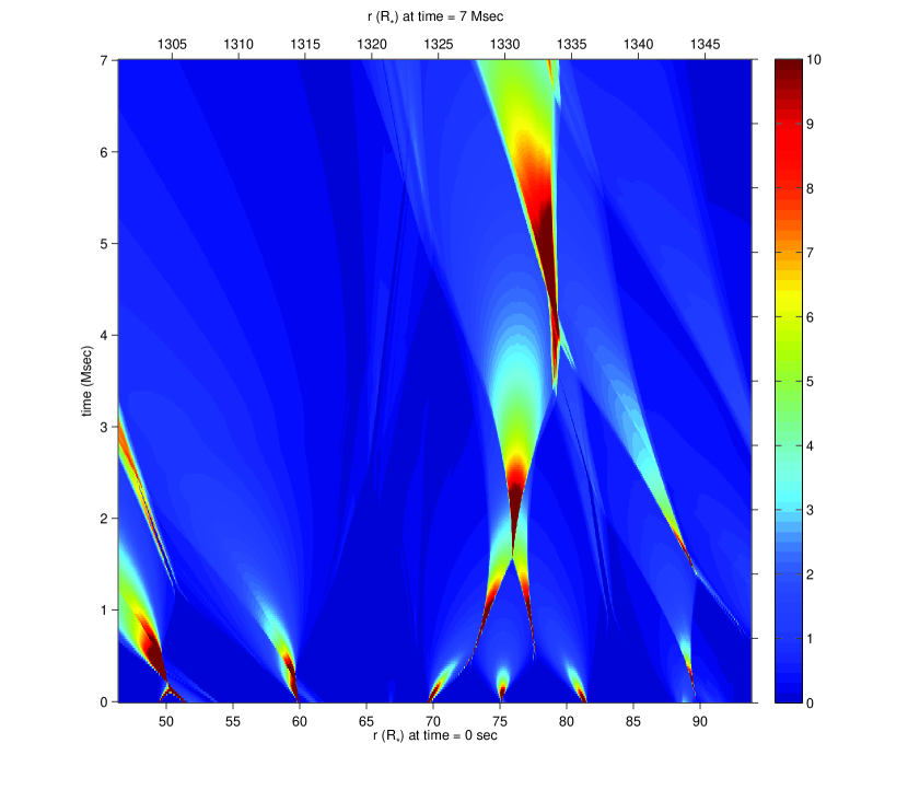
Figure 1: Image of the density contrast as a function of space and time. The intensity scale has been truncated to highlight the kinematics of the shells. The adopted model parameters are the same as in Runacres & Owocki ([2005]).

The clumping factor for a moving-box model extending out to $\sim 1300\leavevmode\nobreak\ R_{*}$ is shown in Fig. 2.

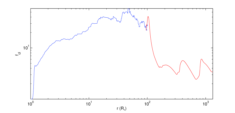
Figure 2: The clumping factor as a function of radius, predicted by our theoretical models. Below 100 $R_{*}$ the model is a line-driven instability model, above $100\leavevmode\nobreak\ R_{*}$ it is a moving-box model.

Below 100 $R_{*}$ the model is a line-driven instability model, above $100\leavevmode\nobreak\ R_{*}$ it is a moving-box model. It is clear that these models predict that the winds stays clumped well into the radio formation region, with clumping factors beyond $200\leavevmode\nobreak\ R_{*}$ ranging from 2.5 to 6. Inferred mass-loss rates would therefore be overestimated by a factor of two.

4 Discussion and conclusions

Our models predict an increase of the clumping factor from the base of the wind to $\sim 50\leavevmode\nobreak\ R_{*}$ (Fig. 2), after which the clumping factor decreases, maintaining a level of residual clumping beyond $200\leavevmode\nobreak\ R_{*}$. This does not quite match the clumping factors derived from observations by Puls et al. ([2006]), which start to tail off closer to the star ($\sim 10\leavevmode\nobreak\ R_{*}$). As has been mentioned before, the observations do not tell us whether or not there is residual clumping at very large distances from the star.

There are of course a number of limitations to our model. As has been mentioned above, we have used self-excited structure without external perturbations. Also, we have not attempted to model different spectral types. In particular, the important difference between dense and less dense winds found by Puls et al. ([2006]) has not been investigated at all in our models.

A key limitation of the present model is of course its restriction to just one dimension. The focus here is entirely on the extensive radial structure, and the instabilities that are likely to break up the azimuthal coherence of the structure are not accounted for. It remains to be seen to what extent this changes the global evolution of instability-generated wind structure. We plan to extend the present models to 2-D in the near future.

References

- 1991 Owocki, S. P. 1991, in Stellar Atmospheres : Beyond Classical Models, ed. L. Crivellari, I. Hubeny & D. G. Hummer (Dordrecht : Kluwer), 235
- 1984 Owocki, S. P., & Rybicki, G. B. 1984, ApJ, 284, 337
- 1998 Prinja, R.K.. 1998, in Cyclical Variability in Stellar Winds, ed. L. Kaper & A. W. Fullerton (Garching: ESO)
- 2006 Puls, J., Markova, N., Scuderi, S., Stanghellini, C., Taranova, O. G., Burnley, A. W., & Howarth, I. D. 2006, A&A, 454, 625
- 2002 Runacres, M. C., & Owocki, S. P. 2002, ApJ, 381, 1015
- 2005 Runacres, M. C., & Owocki, S. P. 2005, ApJ, 429, 323