Dynamical Barrier for the Formation of Solitary Waves in Discrete Lattices

Abstract

We consider the problem of the existence of a dynamical barrier of “mass” that needs to be excited on a lattice site to lead to the formation and subsequent persistence of localized modes for a nonlinear Schrödinger lattice. We contrast the existence of a dynamical barrier with its absence in the static theory of localized modes in one spatial dimension. We suggest an energetic criterion that provides a sufficient, but not necessary, condition on the amplitude of a single-site initial condition required to form a solitary wave. We show that this effect is not one-dimensional by considering its two-dimensional analog. The existence of a sufficient condition for the excitation of localized modes in the non-integrable, discrete, nonlinear Schrödinger equation is compared to the dynamics of excitations in the integrable, both discrete and continuum, version of the nonlinear Schrödinger equation.

I Introduction

In the past few years, there has been an explosion of interest in discrete models that has been summarized in numerous recent reviews reviews . This growth has been spurted by numerous applications of dynamical lattice nonlinear models in areas as diverse as the nonlinear optics of waveguide arrays optics , the dynamics of Bose-Einstein condensates in periodic potentials bec_reviews , micro-mechanical models of cantilever arrays sievers , or even simple models of the complex dynamics of the DNA double strand peyrard . Perhaps the most prototypical model among those that emerge in these settings is the, so-called, discrete nonlinear Schrödinger equation (DNLS) dnls . DNLS may arise as a direct model, as a tight binding approximation, or even as an envelope wave expansion: it is, arguably, one of the most ubiquitous models in the nonlinear physics of dispersive, discrete systems.

In at least one of these settings (namely, in the nonlinear optics of waveguide arrays with the focusing nonlinearity), the feature that will be of interest to the present work has been observed experimentally. In particular, it has been noted, to the best of our knowledge firstly in Ref. mora , that when an injected beam of light into one waveguide had low intensity, then the beam dispersed through quasi-linear propagation. On the other hand, in the same work, experiments with high intensity of the input beam led to the first example of formation of discrete solitary waves in waveguide arrays. A very similar “crossover” from linear to nonlinear behavior was also observed very recently in arrays of waveguides with the defocusing nonlinearity rosberg . The common feature of both works is that they used the DNLS equation as the supporting model to illustrate this behavior at a theoretical/numerical level. However, this crossover phenomenon is certainly not purely discrete in nature. Perhaps the most famous example of a nonlinear wave equation that possesses such a threshold is the integrable continuum nonlinear Schrödinger equation sulem . Specifically, it is well-known that, e.g., in the case of a square barrier of initial conditions of amplitude $V_{0}$ and width $L$, the product $V_{0}L$ determines the nature of the resulting soliton, and if it is sufficiently small the initial condition disperses without the formation of a solitonic structure ZS . On the other hand, the existence of the threshold is not a purely one-dimensional feature either. For instance, experiments on the formation of solitary waves in two-dimensional photorefractive crystals show that low intensities lead to diffraction, whereas higher intensities induce localization neshev ; fleischer . Moreover, similar phenomena were observed even in the formation of higher-order excited structures such as vortices (as can be inferred by carefully inspecting the results of Refs. neshev2 ; fleischer2 ). It should be mentioned that the latter field of light propagation in photorefractive crystals is another major direction of current research in nonlinear optics; see, e.g., Ref. moti for a recent review.

This crossover behavior between linear and nonlinear dynamics may be understood qualitatively rather simply. In the case of power law nonlinearities of order $p$, which are relevant in these settings, a small intensity O$(\epsilon)$, where $\epsilon\ll 1$, yields a nonlinear contribution O$(\epsilon^{p})$ that is negligible with respect to the linear terms of the equation. On the other hand, if $\epsilon\gg 1$, the opposite will be true and the nonlinear terms will dominate the linear ones, yielding essentially nonlinear behavior. A key question regards the details of this crossover and what determines its more precise location for an appropriately parametrized initial condition. This is the question we address herein. We argue that the problem related to the experiments described above reduces, at the mathematical level, to a DNLS equation with a Kronecker-$\delta$ initial condition parametrized by its amplitude. Then, a well defined value of the initial-state amplitude exists such that initial states with higher amplitude always give rise to localized modes. The condition may be determined by comparing the energy of the initial state with the energy of the localized excitations that the model supports. This sufficient, but not necessary, condition for the formation of localized solitary waves provides an intuitively and physically appealing interpretation of the dynamics that is in very good agreement with our numerical observations. We also consider variants of this process in different settings: for reasons of completeness, we present it also in the continuum NLS equation, noting the significant differences that the latter case has from the present one. As yet another example of very different (from both its non-integrable sibling and its continuum limit) dynamical behavior, we also present the case of the integrable discrete NLS (so-called Ablowitz-Ladik al1 ; al2 ; trub ) model. In addition to the one-dimensional DNLS lattice, we also consider the two-dimensional case where the role of both energy and beam power (mathematically the squared $l^{2}$-norm) become apparent. We should note here that our tool of choice for visualizing the “relaxational process” (albeit in a Hamiltonian system) of the initial condition will be energy-power diagrams. Such diagrams have proven very helpful in visualizing the dynamics of initial conditions in a diverse host of nonlinear wave equations. In particular, they have been used in the nonlinear homogeneous systems such as birefringent media and nonlinear couplers as is discussed in Chapters 7 and 8 of Ref. akm1 . They have also been used in a form closely related to the present work (but in the continuum case; see also the discussion below) for general nonlinearities in dispersive wave equations in akm2 , while they have been used to examine the migration of localized excitations in DNLS equations in rumpf .

Our presentation is structured as follows. In section II, we present the analytically tractable theory of the integrable “relatives” of the present model: we review the known theory for the NLS model and develop its analog for the integrable discrete NLS case. Then, in section III, we present our analytical and numerical results in the one- and two-dimensional DNLS equation. In the last section, we summarize our findings and present our conclusions, as well as highlight some important questions for future studies.

II Threshold Conditions for the Integrable NLS Models

II.1 The Continuum NLS Model

For reasons of completeness of the presentation and to compare and contrast the results of the non-integrable case that is at the focus of the present work, we start by summarizing the threshold conditions for the continuum NLS model ZS . For the focusing NLS equation

$$iu_{t}=-\frac{1}{2}u_{xx}-|u|^{2}u,$$ (1)

with squared barrier initial data

$$u(x,0)=\left\{\!\begin{array}[]{cc}V_{0},&-L\leq x\leq L\\ 0,&\mbox{otherwise}\end{array}\!\right.,$$ (2)

(the inverse of) the transmission coefficient, $S_{11}(E)$, which is the first entry of the scattering matrix, is given by

$$S_{11}(E)=\nu(E)\cos(2\nu(E)L)-iE\sin(2\nu(E)L),$$ (3)

with $\nu(E)=\sqrt{E^{2}+V_{0}^{2}}$ where $E$ is the spectral parameter and $V_{0}$ the amplitude of the barrier. It is well-known that the number of zeros of this coefficient represents the number of solitons produced by the square barrier initial condition ZS .

It can be proved that the roots of this equation are purely imaginary. (This initial condition satisfies the single-lobe conditions of Klaus-Shaw potentials, from which it follows that the eigenvalues are purely imaginary klaus2 ). Let us define $\eta\geq 0$ and use $E=i\eta.$ Then, Eq. (3) becomes

$$\sqrt{1-\eta^{2}}\cos\Big{(}2V_{0}\sqrt{1-\eta^{2}}L\Big{)}+\eta\sin\Big{(}2V_{0}\sqrt{1-\eta^{2}}L\Big{)}=0.$$ (4)

We can verify that Eq. (4) does not have any roots (i.e., leads to no solitons in Eq. (1)) if

$$V_{0}<\frac{\pi}{2}.$$ (5)

Furthermore, the condition to generate $n$ solitons, i.e., so that Eq. (4) has $n$ roots is

$$(2n-1)\frac{\pi}{2}<2V_{0}L<(2n+1)\frac{\pi}{2},$$ (6)

or, equivalently, the count of eigenvalues is given by

$$\frac{2}{\pi}V_{0}L-\frac{1}{2}<n<\frac{2}{\pi}V_{0}L+\frac{1}{2}.$$ (7)

The limit $V_{0}\rightarrow\infty$ together with $L\rightarrow 0$ can be reached if we impose $2V_{0}L={\rm const}.$ In this instance, the number of eigenvalues stays the same.

II.2 The Ablowitz-Ladik Model

We now turn to the integrable discretization of Eq. (1) and examine its dynamics. The one-dimensional integrable, discrete nonlinear Schrödinger model (so-called Ablowitz-Ladik (AL) model al1 ; al2 ; trub ) reads:

$$i\dot{u}_{n}=-\frac{1}{2}(u_{n+1}+u_{n-1}-2u_{n})-\frac{1}{2}|u_{n}|^{2}\left(u_{n+1}+u_{n-1}\right).$$ (8)

In this case, there exists a Lax pair of linear operators al1 ; al2 ; trub

$${\mathcal{L}}_{n} = Z+M_{n},$$ (9)

$${\mathcal{B}}_{n} = \left(\frac{z-z^{-1}}{2}\right)^{2}D+\frac{1}{2}\left({ZM_{n}-Z^{-1}M_{n-1}}\right)-\frac{1}{2}DM_{n}M_{n-1},$$ (10)

with the definitions for the matrices

$$Z=\left(\!\begin{array}[]{cc}z&0\\ 0&z^{-1}\end{array}\!\right),\hskip 14.22636ptD=\left(\!\begin{array}[]{cc}-1&0\\ 0&1\end{array}\!\right),\hskip 14.22636pt\mbox{and}\hskip 14.22636ptM_{n}=\left(\!\begin{array}[]{ccc}0&U_{n}\\ -U_{n}^{\star}&0\end{array}\!\right),$$ (11)

where $z$ is the spectral parameter, and $U_{n}=U_{n}(t)$ is a solution of the equation. These two operators (9) and (10) define the system of differential-difference equations

$$\Psi_{n+1} = {\mathcal{L}}_{n}\Psi_{n},$$ (12)

$$i\frac{d}{d\tau}\Psi_{n} = {\mathcal{B}}_{n}\Psi_{n},$$ (13)

for a complex matrix function $\Psi_{n}$. Then, the compatibility condition of Eqs. (12) and (13)

$$i\frac{d}{d\tau}\Psi_{n+1}=i\left.\left(\frac{d}{d\tau}\Psi_{m}\right)\right|_{m=n+1}$$

(i.e., the Lax equation) becomes the AL model. $U_{n}=U_{n}(t)$ is referred to as the potential of the AL eigenvalue problem.

For $U_{n}$ decaying rapidly at $\pm\infty$, and for $n\rightarrow\pm\infty$, from Eq. (12) we have:

$$\Psi_{n+1}\sim Z\Psi_{n}.$$

We normalize this type of solutions as follows: let $\Psi_{n}$ denote the solution of Eq. (12) such that

$$\Psi_{n}\sim Z^{n}\hskip 28.45274pt\mbox{as}\hskip 28.45274ptn\rightarrow+\infty,$$

and let $\Phi_{n}$ be the solution of Eq. (12) such that

$$\Phi_{n}\sim Z^{n}\hskip 28.45274pt\mbox{as}\hskip 28.45274ptn\rightarrow-\infty.$$

$\Psi_{n}$ and $\Phi_{n}$ are known as the Jost functions. Each of these forms a system of linearly independent solutions of the AL eigenvalue problem (12). These sets of solutions are inter-related by the scattering matrix $S(z)$,

$$\Phi_{n}=\Psi_{n}S(z).$$ (14)

The first column of this equation is given by

$$(\Phi_{1})_{n}=S_{11}(z)(\Psi_{1})_{n}+S_{21}(z)(\Psi_{2})_{n},$$ (15)

where $(\Phi_{1})_{n}$ denotes the first column of $\Phi_{n}$. Similar definitions apply to $(\Psi_{1})_{n}$ and $(\Psi_{2})_{n}$. Since $\Phi_{n}\sim Z^{n}$ as $n\rightarrow-\infty$, then

$$(\Phi_{1})_{n}\sim z^{n}\left(\!\begin{array}[]{c}1\\ 0\end{array}\!\right).$$

To obtain decay, $(\Phi_{1})_{n}\rightarrow 0$ when $n\rightarrow-\infty$, we demand

$$|z|>1.$$ (16)

On the other hand,

$$\Psi_{n}=((\Psi_{1})_{n},(\Psi_{2})_{n})\sim\left(\!\begin{array}[]{cc}z^{n}&0\\ 0&z^{-n}\end{array}\!\right)\hskip 28.45274pt\mbox{as}\hskip 28.45274ptn\rightarrow\infty.$$

Therefore, if $|z|>1$ then $(\Psi_{1})_{n}\rightarrow\infty$ and $(\Psi_{2})_{n}\rightarrow 0$, as $n\rightarrow\infty$. Now, from Eq. (15) it follows that $(\Phi_{1})_{n}\rightarrow\infty$ as $n\rightarrow\infty,$ unless $S_{11}(z)=0.$

We therefore seek solutions $z_{1},z_{2},\ldots,z_{N}$ of the equation

$$S_{11}(z_{k})=0,\hskip 28.45274ptk=1,2,\ldots,N,$$ (17)

such that $|z_{k}|>1$. Then,

$$(\Phi_{1})_{n}(z_{k})=S_{21}(z_{k})(\Psi_{2})_{n}(z_{k}),\hskip 28.45274ptk=1,2,\ldots,N.$$

From this, it follows that $(\Phi_{1})_{n}(z_{k})$ decays at $\pm\infty$:

$$(\Phi_{1})_{n}(z_{k})\rightarrow 0\hskip 28.45274pt\mbox{as}\hskip 28.45274ptn\rightarrow\pm\infty.$$

It is then said that $(\Phi_{1})_{n}(z_{k})$ is an eigenfunction ($k=1,2,\ldots,N$), with corresponding eigenvalue $z_{k}$.

In the case of $U_{n}(t=0)=U_{0}\delta_{n,n_{0}}$, the Jost function is

$$\Phi_{n}=Z^{n-1}(Z+M_{0})\Phi_{0},\hskip 14.22636pt\mbox{for}\hskip 14.22636ptn\geq 1,$$ (18)

with $M_{0}$

$$M_{0}=\left(\!\begin{array}[]{ccc}0&U_{0}\\ -U_{0}&0\end{array}\!\right).$$ (19)

Furthermore, $\Psi_{n}=Z^{n}$ for $n\geq 1$ and $\Phi_{0}$ is the identity matrix: $\Phi_{0}=I$. Hence, Eq. (18) reads:

$$\Phi_{n}=\Psi_{n}Z^{-1}(Z+M_{0}),\hskip 14.22636pt\mbox{for}\hskip 14.22636ptn\geq 1.$$

Its comparison with Eq. (14) leads to a scattering matrix

$$S(z)=Z^{-1}(Z+M_{0}).$$

We thus obtain that the transmission coefficient

$$S_{11}(z)=1,$$

which never vanishes. This means that the one-site potential (i.e., a single-site initial condition) does not admit solitonic solutions, independently of the amplitude $U_{0}$ of initial excitation. This theoretical result has also been confirmed by numerical simulations for different values of $U_{0}$, always leading to dispersion of the solution (not shown here).

III Threshold Conditions for the Non-Integrable DNLS Model

We now turn to the non-integrable DNLS lattice that has the general form:

$$i\dot{u}_{n}=-\epsilon\Delta_{2}u_{n}-|u_{n}|^{2\sigma}u_{n},$$ (20)

where $u_{n}$ is a complex field (corresponding to the envelope of the electric field in optics, or the mean field wavefunction in optical lattice wells in the BECs), $\Delta_{2}u_{n}=(u_{n+1}+u_{n-1}-2u_{n})$ is the discrete Laplacian, and $\epsilon$ is the ratio of the tunneling strength to the nonlinearity strength. Using a scaling invariance of the equation, we can scale $\epsilon=1$, through rescaling $t\rightarrow\epsilon t$ and $u_{n}\rightarrow u_{n}/\sqrt{\epsilon}$. Importantly for our considerations, this model has an underlying Hamiltonian (which is also a conserved quantity in the dynamics) of the form:

$$H=\sum_{n}|u_{n+1}-u_{n}|^{2}-\frac{1}{\sigma+1}|u_{n}|^{2\sigma+2}.$$ (21)

The only other known conserved quantity in the dynamics of Eq. (20) is the beam power (in Bose-Einstein condensates, the normalized number of atoms) $P=\sum_{n}|u_{n}|^{2}$.

The specific problem that we examine here addresses the following question. Consider a “compactum” of mass $u_{n}=A\delta_{n,0}$; what is the critical value of $A$ that is necessary for this single-site initial condition to excite a localized mode? That such a threshold definitely exists is illustrated in Fig. 1. The case of the leftmost panel is subcritical, leading to the discrete dispersion of the initial datum. This follows the well-known $t^{-1/2}$ amplitude decay which is implied by the solution of the problem in the absence of the nonlinearity:

$$u_{n}(t)=Ai^{n}J_{n}(2t),$$ (22)

where $J_{n}$ is a Bessel function of order $n$. Notice that this can also be shown to be consistent with the findings of ournon . On the other hand, the rightmost panel shows a nonlinearity-dominated regime with the rapid formation of a solitary wave strongly localized around $n=0$. In the intermediate case of the middle panel, the system exhibits a long oscillatory behavior reminiscent of a separatrix between the basins of attraction of the two different regimes.

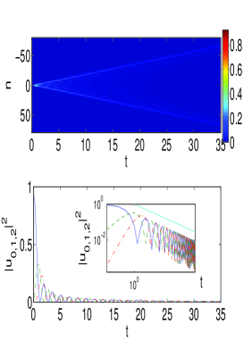
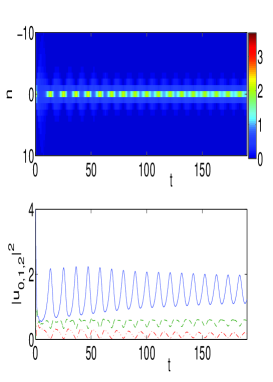
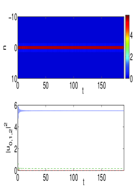
Figure 1: Subcritical case (left), critical (middle), and supercritical (right) initial single-site excitations on the lattice. In all cases, the initial condition is $u_{n}=A\delta_{n,0}$, with $A=1$ in the left, $2$ in the middle, and $2.5$ in the right panels. In each case the top panel shows the space-time contour plot of the evolution. The bottom panel shows the dynamical evolution of $|u_{n}|^{2}$ for sites $n=0,1,2$ (solid, dashed and dash-dotted lines, respectively). For the leftmost case the inset shows the same evolution in a log-log plot and a $t^{-1}$ decay for comparison. Clearly, the damped oscillation of the field modulus has an envelope of $t^{-1/2}$.

We argue herein that the essence of this separatrix lies in the examination of the stationary (localized) states of the model. Such standing wave solutions of the form $u_{n}=\exp(i\Lambda t)v_{n}$, which are exponentially decaying for $v_{n}$ as a function of $n$, can be found for arbitrary frequency $\Lambda$ (and arbitrary power $P$ in one spatial dimension). This is a well-known result in one dimension; see e.g., Ref. johanson . On the other hand, the single-site initial condition discussed above has an energy of:

$$H_{ss}=2A^{2}-\frac{1}{\sigma+1}A^{2\sigma+2},$$ (23)

where the subscript denotes single site. Figure 2 summarizes succinctly the power dependence of the energy for these two cases for $\sigma=1$. Both the energy of the stationary solutions as a function of their power and the single-site energy as a function of single-site power ($P_{ss}=A^{2}$), are shown. Note that the two curves $H_{ss}(P_{ss})$ and $H(P)$ do not intersect (except at the trivial point $H=P=0$) since for $\epsilon\neq 0$ single-site states are not stationary ones.

The examination of Fig. 2 provides information on the existence of a sufficient condition for the formation of a localized mode and on the dynamics of the single-site initial condition. Figure 2 shows that localized solutions exist for arbitrarily small values of the input power $P$, and that the energy of the localized states is negative. This implies that the crucial quantity to determine the fate of the process is the energy $H$ and not the power $P$. The role of the power will become more evident in the two-dimensional setting mentioned below. Moreover, if the system starts at a given point on the curve defined by $H_{ss}=2P_{ss}-P_{ss}^{\sigma+1}/(\sigma+1)$, due to conservation of total $H$ and total $P$, it can only end up in a stationary state in the quadrant $H<H_{ss}$ and $P<P_{ss}$. That is to say, some of the initial energy and power are typically “shed off” in the form of radiation (i.e., converted to other degrees of freedom which is the only way that “effective dissipation” can arise in a purely Hamiltonian system), so that the initial condition can “relax” to the pertinent final configuration. As mentioned above, a localized solution with the same power as that of the initial condition exists for arbitrary $A$. However, emergence of a localized mode occurs only for those initial conditions whose core energy (i.e., the energy of a region around the initially excited state) is negative, after the profile is “reshaped” by radiating away both energy and power.

Therefore, if $H_{ss}<0$, then the compactum of initial data will always yield a localized excitation: this inequality provides the sufficient condition for the excitation of solitary waves. The condition on the energy, in turn, provides a condition on the single-site amplitude that leads to the formation of solitary waves, namely, solitary waves always form if $A>A^{\ast}$ with

$$A^{\ast}=\left[2\left(\sigma+1\right)\right]^{\frac{1}{2\sigma}}.$$ (24)

For the case of $\sigma=1$ considered in Figs. 1 and 2, this amplitude value is $A^{\ast}=2$ in agreement with our numerical observations of Fig. 1. Whether an initial state with $H_{ss}>0$ yields a localized state depends on the explicit system dynamics, corroborating the observation that the previous energetic condition is a sufficient, but not necessary, condition.

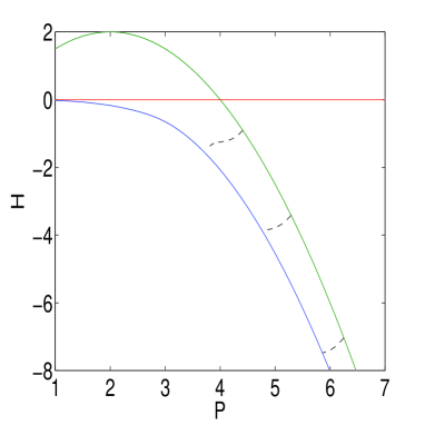
Figure 2: The blue solid line shows the energy $H$ versus the power $P$ of the discrete solitary wave solutions. Above it, the green solid line shows the energy versus power of the initial condition, obtained from Eq. (23) and $P_{ss}=A^{2}$. The horizontal line denotes $H=0$ and its intersection with the initial condition curve defines the single-site, initial amplitude $A^{\ast}$. The dynamical evolution of three different supercritical initial states with $A=2.1$, $A=2.3$, and $A=2.5$ is shown by dashed (black) lines; see also discussion in the text.

One should make a few important observations here. Firstly, we note the stark contrast of the non-integrable discrete model and both of its integrable (continuum and discrete) counterparts. In the (singular) continuum limit, it is possible to excite a single soliton or a multi-soliton depending on the barrier height and width. On the other hand, in the integrable discretization one-site excitation never leads to solitary wave formation, contrary to what is the case here where either none or one solitary wave may arise, depending on the amplitude of the initial one-site excitation.

Restricting our consideration to the non-integrable model, we observe that even though a localized solution with the same power as that of the initial condition exists for arbitrary $A$, formation of a localized mode will always occur only for $A>A^{\ast}$, as determined by the previous energetic criterion. Secondly, the answer that the formation always occurs for $A>A^{\ast}$ generates two interconnected questions: what is the threshold for the formation of the localized mode, and given an initial $A>A^{\ast}$, which one among the mono-parametric family of solutions will the dynamics of the model select as the end state of the system ? [It should be noted in connection to the latter question that single-site initial conditions have always been found in our numerical simulations to give rise to at most a single-site-centered solution i.e., multipulses cannot be produced by this process.] Some examples of this dynamical process are illustrated in Fig. 2, where the energy and power of a few sites (typically 20-40) around the originally excited one are measured as a function of time and are parametrically plotted in the $H-P$ plane. As it should, the relevant curve starts from the $H_{ss}-P_{ss}$ curve, and asymptotically approaches, as a result of the dynamical evolution, the $H-P$ curve of the stationary states of the system. However, the relaxation process happens neither at fixed energy, nor at fixed power. Instead, it proceeds through a more complex, dynamically selected pathway of loss of both $H$ and $P$ to relax eventually to one of the relevant stationary states. This is shown for three different values of super-critical amplitude in Fig. 2 ($A=2.1$, $2.3$ and $2.5$). We have noticed (numerically) that the loss of energy and power, at least in the initial stages of the evolution happens at roughly the same rate, resulting in $dH/dP\approx{\rm const}$. However, the later stages of relaxation no longer preserve this constant slope. It is worthwhile to highlight here that the fact that the process of formation of a localized mode is neither equienergetic, nor does it occur at fixed power is something that has been previously observed in the continuum version of the system in akm2 (cf. with the discussion in p. 6095 therein).

The dynamics of the system in the $H-P$ space can be qualitatively understood by considering the frequencies $\Lambda$ associated with the instantaneous $H$, $P$ values along the system trajectories. At each instantaneous energy $H$ a frequency $\Lambda_{H}$ may be defined as the frequency of a single-site breather stationary state with energy $H$. Such a frequency is unique as the stationary-state energy is a monotonically decreasing function of the frequency johanson . Similarly, a frequency $\Lambda_{P}$ may be uniquely associated with the instantaneous power $P$, i.e., $\Lambda_{P}$ is the frequency of a stationary state with power $P$. Note, however, that the stationary-state power is a monotonically increasing function of $\Lambda$. At the final stationary state where the system relaxes $\Lambda_{H}=\Lambda_{P}=-dH/dP$. Hence, the system trajectories are such that $\Lambda_{H}$ increases (consequently the energy decreases) and $\Lambda_{P}$ decreases (the power decreases). The final stationary state is reached when the two frequencies become equal, the point where they meet depending on their rate of change along the trajectory, i.e., on their corresponding “speeds” along the trajectory. Nevertheless, the precise mechanism of selection of the particular end state (i.e., of the particular “equilibrium $\Lambda$”) that a given initial state will result in remains a formidable outstanding question that would be especially interesting to address in the future.

We now turn to the two-dimensional variant of the above one-dimensional non-integrable lattice. Equation (20) remains the same, but for the two-dimensional field $u_{n,m}$, and the discrete Laplacian becomes the five-point stencil $\Delta_{2}u_{n,m}=(u_{n+1,m}+u_{n-1,m}+u_{n,m+1}+u_{n,m-1}-4u_{n,m})$. For the initial condition $u_{n,m}=A\delta_{n,0}\delta_{m,0}$, the $H_{ss}-P_{ss}$ curve is given by:

$$H_{ss}=4P_{ss}-P_{ss}^{\sigma+1}/(\sigma+1).$$ (25)

In $d$-dimensions the first term would be $2dP_{ss}$. We once again find the branch of standing waves of the equation. While this branch of solutions is also well-known kevrek , there are some important differences with the one-dimensional case. Firstly, a stable and an unstable branch of solutions exists (per the well-known Vakhitov-Kolokolov criterion); in the wedge-like curve indicating the standing waves only the lower energy branch is stable. Furthermore, the maximal energy of the solutions is no longer $H=0$, but finite and positive (in fact, for $\sigma=1$, it is $H_{0}\approx 1.85$). Finally, solutions no longer exist for arbitrarily low powers, but they may only exist above a certain power (often referred to as the excitation threshold excit1 ; excit2 ; excit3 ). We can now appreciate the impact of these additional features in the right panel of Fig. 3. Comparing $H_{ss}$ with $H_{0}$ we find two solutions: one with $A\approx 0.7$ and one with $A\approx 2.73$. However, for the lower one there are no standing wave excitations with the corresponding power (this reveals the role of the power in the higher dimensional problem). Hence, the relevant amplitude that determines the sufficient condition in the two-dimensional case is the latter. Indeed, the case with $A=2.65$ shown in the left panel of Fig. 3 shows spatio-temporal diffraction, while that of $A=2.75$ in the middle panel illustrates robust localization, indicating the super-critical nature of the latter case. Notice that the pathway of the dynamics is presented in the right panel for three super-critical values of $A=2.75$, $A=2.9$ and $A=3.1$. Once again, the dynamics commences on the $H_{ss}-P_{ss}$ curve, as it should, eventually relaxing on the stable standing wave curve. As before, the initial dynamics follows a roughly constant $dH/dP$, but the relaxation becomes more complex at later phases of the evolution.

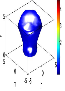
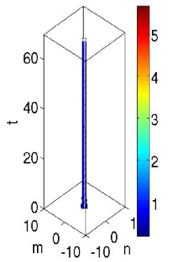
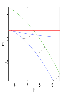
Figure 3: The left panel shows the spatio-temporal evolution of $|u_{n,m}(t)|^{2}$ for the sub-critical case with amplitude $A=2.65$. The middle panel shows the weakly super-critical case of $A=2.75$. Finally the right panel is analogous to Fig. 2, showing the $H-P$ diagram for the solution branch (wedge-like blue solid line), the $H_{ss}-P_{ss}$ graph of the initial conditions (green solid line) and the trajectories of three super-critical cases in $H-P$ space for $A=2.75$, $2.9$ and $3.1$ (dashed black lines). The red horizontal line represents the maximal energy for which solutions are found to exist, namely $H_{0}\approx 1.85$.

IV Conclusions and Future Challenges

The above study has examined the presence of a sharp crossover between the linear and nonlinear dynamics of a prototypical dynamical lattice model such as the discrete nonlinear Schrödinger equation. This crossover has already been observed in media with the focusing nonlinearity mora (as considered here). It has also been observed very recently in media with the defocusing nonlinearity rosberg . The latter can be transformed into the former under the so-called staggering transformation $u_{n}=(-1)^{n}w_{n}$, where $w_{n}$ is the field in the defocusing case. As a result, the solitary waves of the defocusing problem discussed in rosberg will be “staggered” (i.e., of alternating phase between neighboring sites), yet the phenomenology discussed above will persist. The crossover was quantified on the basis of an energetic comparison of the initial-state energy with the branch of corresponding stable localized solutions “available” in the model. A sufficient, but not necessary, condition for the excitation of a localized mode based on the initial-state, single-site amplitude was discussed, and it was successfully tested in numerical simulations. Similar findings were obtained in the two-dimensional analog of the problem: a crossover behaviour dictated by the energy was found, but the crossover was also affected by the power and its excitation thresholds. Furthermore, these results were contrasted with the case of the continuum version of the model, where depending on the strength of the excitation, also multi-solitons can be obtained and with the integrable discrete Ablowitz-Ladik model where no single-site excitation can produce a solitary wave, independently of the excitation amplitude.

However, a number of interesting questions emerge from these findings that are pertinent to future studies. Perhaps the foremost among them concerns how the dynamics “selects” among the available steady-state excitations with energy and power below that of the initial condition the one to which the dynamical evolution leads. According to our results, this evolution is neither equienergetic, nor power-preserving (see also akm2 ), hence it would be extremely interesting to identify the leading physical principle which dictates it. Another question generalizing the more principal one asked herein concerns the excitation of multiple sites (possibly at the same amplitude), starting with two, and inquiring the nature of the resulting state of the system. On a related note, perhaps this last question is most suitable to be addressed first in the context of the integrable model where the formulation presented herein can be generalized and yield definitive answers for the potential excitation of solitons. Studies along these directions are currently in progress and will be reported in future publications.

V Acknowledgements

YD gratefully acknowledges discussions with L. Isella. PGK gratefully acknowledges support from grants NSF-DMS-0505663, NSF-DMS-0619492 and NSF-CAREER.

References

- (1) S. Aubry, Physica D 103, 201, (1997); S. Flach and C.R. Willis, Phys. Rep. 295, 181 (1998); D. Hennig and G. Tsironis, Phys. Rep. 307, 333 (1999);
- (2) D. N. Christodoulides, F. Lederer and Y. Silberberg, Nature 424, 817 (2003); Yu. S. Kivshar and G. P. Agrawal, Optical Solitons: From Fibers to Photonic Crystals, Academic Press (San Diego, 2003).
- (3) V.V. Konotop and V.A. Brazhnyi, Mod. Phys. Lett. B 18, 627 (2004); O. Morsch and M. Oberthaler, Rev. Mod. Phys. 78, 179 (2006); P.G. Kevrekidis and D.J. Frantzeskakis, Mod. Phys. Lett. B 18, 173 (2004).
- (4) M. Sato, B. E. Hubbard, and A. J. Sievers, Rev. Mod. Phys. 78, 137 (2006).
- (5) M. Peyrard, Nonlinearity 17, R1 (2004).
- (6) P.G. Kevrekidis, K.O. Rasmussen, and A.R. Bishop, Int. J. Mod. Phys. B 15, 2833 (2001).
- (7) H.S. Eisenberg, Y. Silberberg, R. Morandotti, A.R. Boyd and J.S. Aitchison, Phys. Rev. Lett. 81, 3383 (1998).
- (8) M. Matuszewski, C.R. Rosberg, D.N. Neshev, A.A. Sukhorukov, A. Mitchell, M. Trippenbach, M.W. Austin, W. Krolikowski and Yu.S. Kivshar, Opt. Express 14, 254 (2006).
- (9) C. Sulem and P.L. Sulem, The Nonlinear Schrödinger Equation, Springer-Verlag (New York, 1999).
- (10) V.E. Zakharov and A.B. Shabat, Soviet Physics-JETP 34, 62 (1972).
- (11) J.W. Fleischer, T. Carmon, M. Segev, N.K. Efremidis and D.N. Christodoulides, Phys. Rev. Lett. 90, 023902 (2003); J.W. Fleischer, M. Segev, N.K. Efremidis and D.N. Christodoulides, Nature 422, 147 (2003).
- (12) H. Martin, E.D. Eugenieva, Z. Chen and D.N. Christodoulides, Phys. Rev. Lett. 92, 123902 (2004).
- (13) D.N. Neshev, T.J. Alexander, E.A. Ostrovskaya, Yu.S. Kivshar, H. Martin, I. Makasyuk and Z. Chen, Phys. Rev. Lett. 92, 123903 (2004).
- (14) J.W. Fleischer, G. Bartal, O. Cohen, O. Manela, M. Segev, J. Hudock and D.N. Christodoulides, Phys. Rev. Lett. 92, 123904 (2004).
- (15) J.W. Fleischer, G. Bartal, O. Cohen, T. Schwartz, O. Manela, B. Freeman, M. Segev, H. Buljan, and N.K. Efremidis, Optics Express 13, 1780 (2005).
- (16) M.J. Ablowitz and J.F. Ladik, J. Math. Phys. 16, 598 (1975).
- (17) M.J. Ablowitz and J.F. Ladik, J. Math. Phys. 17, 1011 (1976).
- (18) M.J. Ablowitz, B. Prinari and A.D. Trubatch, Discrete and Continuous Nonlinear Schrödinger Systems, Cambridge University Press (Cambridge, 2004).
- (19) N.N. Akhmediev and A. Ankiewicz, Solitons: Nonlinear pulses and beams, Chapman & Hall (London 1997).
- (20) N.N. Akhmediev, A. Ankiewicz, and R. Grimshaw, Phys. Rev. E 59, 6088 (1999).
- (21) B. Rumpf, Phys. Rev. E 70, 016609 (2004).
- (22) M. Klaus and J. K. Shaw, Phys. Rev. E 65, 036607 (2002).
- (23) A. Stefanov and P.G. Kevrekidis, Nonlinearity 18, 1841 (2005).
- (24) M. Johansson and S. Aubry, Phys. Rev. E 61, 5864 (2000).
- (25) P. G. Kevrekidis, K. Ø. Rasmussen, and A. R. Bishop, Phys. Rev. E 61, 2006-2009 (2000).
- (26) S. Flach, K. Kladko and R.S. MacKay, Phys. Rev. Lett. 78, 1207 (1997).
- (27) M.I. Weinstein, Nonlinearity 12, 673 (1999).
- (28) P.G. Kevrekidis, K.Ø. Rasmussen and A.R. Bishop, Phys. Rev. E 61, 4652 (2000).