Optimizing the discrete time quantum walk using a $SU(2)$ coin

Abstract

We present a generalized version of the discrete time quantum walk, using the $SU(2)$ operation as the quantum coin. By varying the coin parameters, the quantum walk can be optimized for maximum variance subject to the functional form $\sigma^{2}\approx N^{2}$ and the probability distribution in the position space can be biased. We also discuss the variation in measurement entropy with the variation of the parameters in the $SU(2)$ coin. Exploiting this we show how quantum walk can be optimized for improving mixing time in an $n$-cycle and for quantum walk search.

I Introduction

The discrete time quantum walk has a very similar structure to that of the classical random walk - a coin flip and a subsequent shift - but the behaviour is strikingly different because of quantum interference. The variance $\sigma^{2}$ of the quantum walk is known to grow quadratically with the number of steps $N$, $\sigma^{2}\propto N^{2}$, compared to the linear growth, $\sigma^{2}\propto N$, for the classical random walk aharonov ; kemp ; ashwin ; andris . This has motivated the exploration for a new and improved quantum search algorithms, which under certain conditions are exponentially fast compared to the classical analog childs . Environmental effects on the quantum walk chandra07 and the role of the quantum walk to speed up the physical process, such as the quantum phase transition have been explored chandra07a . Experimental implementation of the quantum walk has been reported ryan and various other schemes for a physical realization have been proposed travaglione .

The quantum walk of a particle initially in a symmetric superposition state $|\Psi_{in}\rangle$ using a single-variable parameter $\theta$ in the unitary operator, $U_{\theta}\equiv\left(\begin{array}[]{clcr}\cos(\theta)&&\sin(\theta)\\ \sin(\theta)&&-\cos(\theta)\end{array}\right)$, as quantum coin returns the symmetric probability distribution in the position space. The change in the parameter $\theta$ is known to affect the variation in the variance, $\sigma^{2}$ ashwin . It has been reported that obtaining a symmetric distribution depends largely on the initial state of the particle ashwin ; andris ; tregenna .

In this paper, the discrete time quantum walk has been generalized using the $SU(2)$ operator with three Caley-Klein parameters $\xi$, $\theta$ and $\zeta$ as the quantum coin. We show that the variance can be varied by changing the parameter $\theta$, $\sigma^{2}\approx(1-\sin(\theta))N^{2}$ and the parameters $\xi$ and $\zeta$ introduce asymmetry in the position-space probability distribution even if the initial state of the particle is in symmetric superposition. This asymmetry in the probability distribution is similar to the distribution obtained for a walk on a particle initially in a non-symmetric superposition state. We discuss the variation of measurement entropy in position space with the three parameters. Thus, we also show that the quantum walk can be optimized for the maximum variance, for applications in search algorithm, improving mixing time in an $n$-cycle or general graph and other processes using a generalized $SU(2)$ quantum coin. The combination of the measurement entropy and three parameters in the $SU(2)$ coin can be optimized to fit the physical system and for the relevant applications of the quantum walk on general graphs. This paper discuss the effect of $SU(2)$ coin on quantum walk with particle initially in symmetric superposition state. The $SU(2)$ coin will have a similar influence on a particle starting with other initial states but with an additional decrease in the variance by a small amount.

The paper is organized as follows. Section II introduces to the discrete time quantum (Hadamard) walk. Section III discusses the generalized version of the quantum walk using the arbitrary three-parameter $SU(2)$ quantum coin. The effect of three parameters on the variance of the quantum walker is discussed, and the functional dependence of the variance due to parameter $\theta$ is shown. The variation of the entropy of the measurement in position space after implementing the quantum walk using different values of $\theta$ is discussed in Sec. IV. Section V and VI discuss optimization of the mixing time of the quantum walker on the $n-$cycle and the search using a quantum walk. Section VII concludes with a summary.

II Hadamard walk

To define the one-dimensional discrete time quantum (Hadamard) walk we require the coin Hilbert space $\mathcal{H}_{c}$ and the position Hilbert space $\mathcal{H}_{p}$. The $\mathcal{H}_{c}$ is spanned by the internal (basis) state of the particle, $|0\rangle$ and $|1\rangle$, and the $\mathcal{H}_{p}$ is spanned by the basis state $|\psi_{i}\rangle$, $i\in\mathbb{Z}$. The total system is then in the space $\mathcal{H}=\mathcal{H}_{c}\otimes\mathcal{H}_{p}$. To implement the simplest version of the quantum walk, known as the Hadamard walk, the particle at origin in one of the basis state is evolved into the superposition of the $\mathcal{H}_{c}$ with equal probability, by applying the Hadamard operation, $H=\frac{1}{\sqrt{2}}\left(\begin{array}[]{clcr}1&&1\\ 1&&-1\end{array}\right)$, such that,

$$(H\otimes\mathbbm{1})(|0\rangle\otimes|\psi_{0}\rangle)=\frac{1}{\sqrt{2}}[|0\rangle+|1\rangle]\otimes|\psi_{0}\rangle$$

$$(H\otimes\mathbbm{1})(|1\rangle\otimes|\psi_{0}\rangle)=\frac{1}{\sqrt{2}}[|0\rangle-|1\rangle]\otimes|\psi_{0}\rangle.$$ (1)

The $H$ is then followed by the conditional shift operation $S$: conditioned on the internal state being $|0\rangle$ ($|1\rangle$) the particle moves to the left (right),

$$S=|0\rangle\langle 0|\otimes\sum_{i\in\mathbb{Z}}|\psi_{i-1}\rangle\langle\psi_{i}|+|1\rangle\langle 1|\otimes\sum_{i\in\mathbb{Z}}|\psi_{i+1}\rangle\langle\psi_{i}|$$ (2)

The operation $S$ evolves the particle into the superposition in position space. Therefore, each step of quantum (Hadamard) walk is composed of an application of $H$ and a subsequent $S$ operator to spatially entangle $\mathcal{H}_{c}$ and $\mathcal{H}_{p}$. The process of $W=S(H\otimes\mathbbm{1})$ is iterated without resorting to the intermediate measurements to realize a large number of steps of the quantum walk. After the first two steps of implementation of $W$, the probability distribution starts to differ from the classical distribution. The probability amplitude distribution arising from the iterated application of $W$ is significantly different from the distribution of the classical walk. The particle with initial coin state $|0\rangle$ ($|1\rangle$) drifts to the right (left). This asymmetry arises from the fact that the Hadamard operation treats the two states $|0\rangle$ and $|1\rangle$ differently, multiplies the phase by $-1$ only in case of state $|0\rangle$. To obtain left-right symmetry in the probability distribution, (b) in Fig. (1 b), one needs to start the walk with the partilce in the symmetric superposition state of the coin, $|\Psi_{in}\rangle\equiv\frac{1}{\sqrt{2}}[|0\rangle+i|1\rangle]\otimes|\psi_{0}\rangle$.

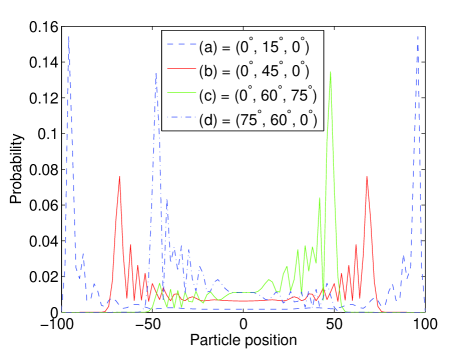
Figure 1: The spread of probability distribution for different value of $\theta$ using operator $U_{0,\theta,0}$, is wider for (a) = $(0,\frac{\pi}{12},0)$ than compared to (b) = $(0,\frac{\pi}{4},0)$. Biasing the walk using $\zeta$ shifts the distribution to right, (c) = $(0,\frac{\pi}{3},\frac{5\pi}{12})$ and $\xi$ shifts to the left, (d) = $(\frac{5\pi}{12},\frac{\pi}{3},0)$. The distribution is for 100 steps.

III Generalized discrete time quantum walk

The coin toss operation in general can be written as an arbitrary three parameter $SU(2)$ operator of the form,

$$U_{\xi,\theta,\zeta}\equiv\left(\begin{array}[]{clcr}e^{i\xi}\cos(\theta)&&e^{i\zeta}\sin(\theta)\\ e^{-i\zeta}\sin(\theta)&&-e^{-i\xi}\cos(\theta)\end{array}\right),$$ (3)

the Hadamard operator, $H=U_{0,\frac{\pi}{4},0}$. By replacing the Hadamard coin with an operator $U_{\xi,\theta,\zeta}$, we obtain the generalized quantum walk. For the analysis of the generalized quantum walk we consider the symmetric superposition state of the particle at the origin. By varying the parameter $\xi$ and $\zeta$ the results obtained for walker starting with one of the basis (or other nonsymmetric superposition) state can be reproduced. A particle at origin in a symmetric superposition state $|\Psi_{in}\rangle$, when subjected to a subsequent iteration of $W_{\xi,\theta,\zeta}=S(U_{\xi,\theta,\zeta}\otimes{\mathbbm{1}})$ implements a generalized discrete time quantum walk on a line. Consider an implementation of $W_{\xi,\theta,\zeta}$, which evolves the walker to,

$$W_{\xi,\theta,\zeta}|\Psi_{in}\rangle=\frac{1}{\sqrt{2}}[\left(e^{i\xi}\cos(\theta)+ie^{i\zeta}\sin(\theta)\right)|0\rangle|\psi_{-1}\rangle$$

$$+\left(e^{-i\zeta}\sin(\theta)-ie^{-i\xi}\cos(\theta)\right)|1\rangle|\psi_{+1}\rangle].$$ (4)

If $\xi=\zeta$, Eq. (III) has left-right symmetry in the position probability distribution, but not otherwise. We thus find that the generalized $SU(2)$ operator as a quantum coin can bias a quantum walker in spite of the symmetry of initial state of the particle. We return to this point below.

It is instructive to consider the extreme values of the parameters in the $U_{\xi,\theta,\zeta}$. If $\xi=\theta=\zeta=0$, $U_{0,0,0}=Z$, the Pauli $Z$ operation, then $W_{\xi,\theta,\zeta}\equiv S$ and the two superposition states, $|0\rangle$ and $|1\rangle$, move away from each other without any diffusion and interference having high $\sigma^{2}=N^{2}$ . On the other hand, if $\theta=\frac{\pi}{2}$, then $U_{0,\frac{\pi}{2},0}=X$, the Pauli $X$ operation, then the two states cross each other going back and forth, thereby remaining close to position $i=0$ and hence giving very low $\sigma^{2}\approx 0$. These two extreme case are not of much importance, but they define the limits of the behavior. Intermediate values of the $\theta$ between these extremes show intermediate drifts and quantum interference.

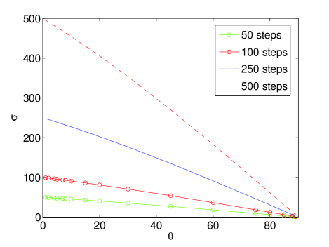
Figure 2: A comparison of variation of $\sigma$ with $\theta$ for different number of steps of walk using operator $U_{0,\theta,0}$ using numerical integration.

In Fig. (1) we show the symmetric distribution of quantum walk at different values of $\theta$ by numerically evolving the density matrix. Fig. (2) shows the variation of $\sigma$ with increase in $\theta$ for quantum walk of different number steps with the operator, $U_{0,\theta,0}$. The change in the variance for different value of the $\theta$ is attributed to the change in the value of $C_{\theta}$, a constant for a given $\theta$, $\sigma^{2}=C_{\theta}N^{2}$, Fig. (4). Therefore, starting from the Hadamard walk ($\theta=\frac{\pi}{4};\xi=\zeta=0$), the variance can be increased ($\theta<\frac{\pi}{4}$) or decreased ($\theta>\frac{\pi}{4}$) respectively.

In the analysis of Hadamard walk on the line in andris , it is shown that after $N$ steps, the probability distributed is spread over the interval $[\frac{-N}{\sqrt{2}},\frac{N}{\sqrt{2}}]$ and shrink quickly outside this region. The moments have been calculated for asymptotically large number of steps $N$ and the variance is shown to vary as $\sigma^{2}(N)=\left(1-\frac{1}{\sqrt{2}}\right)N^{2}$ andris .

The expression for the variance of the quantum walk using $U_{0,\theta,0}$ as a quantum coin can be derived by using the approximate analytical function for the probability distribution $P(i)$ that fit the envelop of the quantum walk distribution obtained from the numerical integration technique for different values of $\theta$. For a quantum walk using $U_{0,\theta,0}$ as quantum coin, after $N$ steps the probability distribution is spread over the interval $(-N\cos(\theta),N\cos(\theta))$ ashwin . This is also verified by the analyzing the distribution obtained using the numerical integration technique. By assuming the value of the probability to be $0$ beyond $|N\cos(\theta)|$, the function that fits the probability distribution envelop is,

$$\int P(i)di\approx$$

$$\int_{-N\cos(\theta)}^{N\cos(\theta)}\frac{[1+\cos^{2}(2\theta)]e^{K(\theta)\left(\frac{i^{2}}{N^{2}\cos^{2}(\theta)}-1\right)}}{\sqrt{N}}di\approx 1,$$ (5)

where, $K(\theta)=\frac{\sqrt{N}}{2}\cos(\theta)[1+\cos^{2}(2\theta)][1+\sin(\theta)]$ notes . Fig. (3) shows the probability distribution obtained by using the Eq. (5).

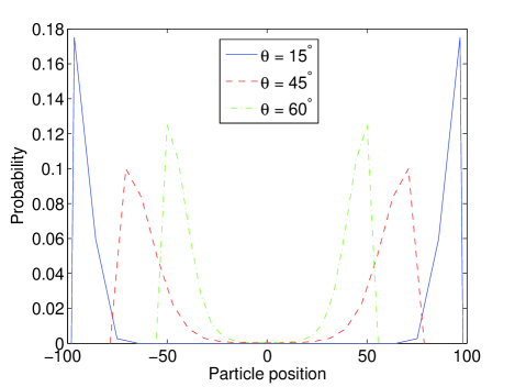
Figure 3: The probability distribution obtained using using Eq. (5) for different value of $\theta$. The distribution is for 100 steps.

The interval $(-N\cos(\theta),N\cos(\theta))$ can be parametrised as a function of $\phi$, $i=f(\phi)=N\cos(\theta)\sin(\phi)$ where $\phi$ range from $-\frac{\pi}{2}$ to $\frac{\pi}{2}$. For a walk with coin $U_{0,\theta,0}$, the mean of the distribution is zero and hence the variance can be analytically obtained by evaluating,

$$\sigma^{2}\approx\int_{-N\cos(\theta)}^{N\cos(\theta)}P(i)i^{2}di=\int_{-\frac{\pi}{2}}^{\frac{\pi}{2}}P(f(\phi))(f(\phi))^{2}f^{\prime}(\phi)d\phi.$$ (6)

$$\sigma^{2}\approx\int_{-\frac{\pi}{2}}^{\frac{\pi}{2}}\frac{(1+\cos^{2}(2\theta))}{\sqrt{N}}{e^{K(\theta)\left(\sin^{2}(\phi)-1\right)}}\left(N\cos(\theta)\sin(\phi)\right)^{2}$$

$$\times\left(N\cos(\theta)\cos(\phi)\right)d\phi=N^{2}(1-\sin(\theta)).$$ (7)

$$\sigma^{2}=C_{\theta}N^{2}\approx(1-\sin(\theta))N^{2}.$$ (8)

We also verify from the results obtained through numerical integration that $C_{\theta}=(1-\sin(\theta))$, Fig. (4).

Figure 4: Variation of $C_{\theta}$ when $\eta=\lvert\xi-\zeta\rvert=0^{\circ}$ from numerical integration to the function $(1-\sin(\theta))$ to which it fits. The effect of maximum biasing, $\eta=90^{\circ}$ on $C_{\theta}$ is also shown and its effect is very small.

Setting $\xi\neq\zeta$ in $U_{\xi,\theta,\zeta}$ introduces asymmetry, biasing the walker. Positive $\zeta$ contributes for constructive interference towards right and destructive interference to the left, whereas vice versa for $\xi$. The inverse effect can be noticed when the $\xi$ and $\zeta$ are negative. As noted above, for $\xi=\zeta$, the evolution will again lead to the symmetric probability distribution. Apart from a global phase, one can show that the coin operator

$$U_{\xi,\theta,\zeta}\equiv U_{\xi-\zeta,\theta,0}\equiv U_{0,\theta,\zeta-\xi}.$$ (9)

In Fig. (1) we show the biasing effect for $(\xi,\theta,\zeta)=(0^{\circ},60^{\circ},75^{\circ})$ and for $(75^{\circ},60^{\circ},0^{\circ})$. The biasing does not alter the width of the distribution in the position space but probability goes down as a function of $\cos(\eta)$ on one side and up as a function of $\sin(\eta)$ on the other side. Where $\eta=\lvert\xi-\zeta\rvert$ . The mean value $\bar{i}$ of the distribution, which is zero for $U_{0,\theta,0}$, attains some finite value with non-vanishing $\eta$, this contributes for an additional term in Eq. (6),

$$\sigma^{2}\approx\int_{-N\cos(\theta)}^{N\cos(\theta)}P(i)(i-\bar{i})^{2}di.$$ (10)

this contributes to a small decrease in the variance of the biased quantum walker, Fig. (4).

It is understood that, obtaining symmetric distribution depends largely on the initial state of the particle and this has also been discussed in ashwin ; andris ; tregenna ; konno . But using $U_{\xi,\theta,\zeta}$ as coin operator, and examining the walk evolution shows how non-vanishing $\xi$ and $\zeta$ introduce bias. For example, the position probability distribution in Eq. (III) corresponding to the left and right positions are $\frac{1}{2}[1\pm\sin(2\theta)\sin(\xi-\zeta)]$, which would be equal, and lead to a symmetric distribution, if and only if $\xi=\zeta$. The evolution of the state after $n$ steps, $[W_{\xi,\theta,\zeta}]^{n}|\Psi_{in}\rangle$ is

$$|\Psi(n)\rangle=\sum_{m=-n}^{n}(A_{m,n}|0\rangle|\psi_{m}\rangle+B_{m,n}|1\rangle|\psi_{m}\rangle)$$ (11)

and proceeds according to the iterative relations,

$$A_{m,n}=e^{i\xi}\cos\theta A_{m-1,n-1}+e^{i\zeta}\sin\theta B_{m-1,n-1}$$ (12a)

$$B_{m,n}=e^{-i\zeta}\cos\theta A_{m-1,n-1}-e^{-i\xi}\sin\theta B_{m-1,n-1}.$$ (12b)

A little algebra reveals that the solutions $A_{m,n}$ and $B_{m,n}$ to Eqs. (12) can be decoupled (after the initial step) and shown to satisfy

$$A_{m,n+1}-A_{m,n-1}=\cos\theta(e^{i\zeta}A_{m-1,n}-e^{i\xi}A_{m+1,n})$$ (13a)

$$B_{m,n+1}-B_{m,n-1}=\cos\theta(e^{i\xi}B_{m-1,n}-e^{i\zeta}B_{m+1,n}).$$ (13b)

For spatial symmetry from an initially symmetric superposition, the walk should be invariant under an exchange of labels $0\leftrightarrow 1$, and hence should evolve $A_{m,n}$ and $B_{m,n}$ alike (as in the Hadamard walk kni03 ). From Eq. (13), we see that this happens if and only if $\xi=\zeta$.

IV Entropy of measurement

As an alternative measure of position fluctuation to variance, we consider the Shannon entropy of the walker position probability distribution $p_{i}$ obtained by tracing over the coin basis:

$$H(i)=-\sum_{i}p_{i}\log p_{i}.$$ (14)

Figure 5: Variation of entropy of measurement $H(i)$ with $\theta$ for different number of steps. The decrease in $H(i)$ is not drastic till $\theta$ is close to $0$ or $\frac{\pi}{2}$.

The quantum walk with a Hadamard coin toss, $U_{0,\frac{\pi}{4},0}$, has the maximum uncertainty associated with the probability distribution and hence the measurement entropy is maximum. For $\xi=\zeta=0$ and low $\theta$, operator $U_{0,\theta,0}$ is almost a Pauli $Z$ operation, leading to localization of walker at $\pm N$. At $\theta$ close to $\frac{\pi}{2}$, with $\xi=\zeta=0$, $U$ approaches Pauli $X$ operation, leading to localization close to the origin, and again, low entropy. However, as $\theta$ approaches $\frac{\pi}{4}$, the splitting of amplitude in position space increases towards the maximum. The resulting enhanced diffusion is reflected in the relatively large entropy at $\frac{\pi}{4}$, as seen in Fig. (5). Fig. (5) is the measurement entropy with variation of $\theta$ in the coin $U_{0,\theta,0}$ for different number of steps of quantum walk. The decrease in entropy from the maximum by changing $\theta$ on either side of $\frac{\pi}{4}$ is not drastic untill the $\theta$ is close to $0$ or $\frac{\pi}{2}$. Therefore for many practical purposes, the small entropy can be compensated for by the relatively large $C_{\theta}$, and hence $\sigma^{2}$. For many other purposes, such as mixing of quantum walk on an $n$-cycle Cayley graph, it is ideal to adopt a lower value of $\theta$. The effect of $\xi$ and $\zeta$ on the measurement entropy is of very small magnitude. These parameters do not affect the spread of the distribution and the variation in the height reduces the entropy by a very small fraction.

V Quantum walk on the $n$-cycle and mixing time

The $n$-cycle is the simplest finite Cayley graph with $n$ vertices. This example has most of the features of the walks on the general graphs.

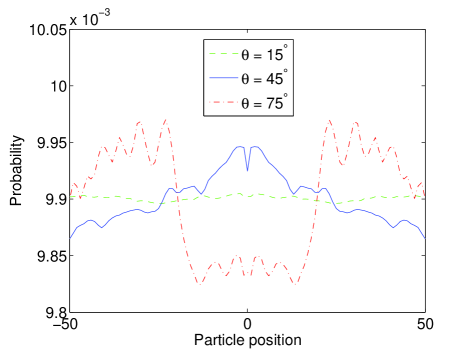
Figure 6: A comparison of mixing time $M$ of the probability distribution of a quantum walker on a $n$-cycle for different value of $\theta$ using coin operation $U_{0,\theta,0}$, where $n$, the number of position, is $101$. Mixing is faster for lower value of $\theta$. The distribution is for 200 cycles.

The classical random walk approaches a stationary distribution independent of its initial state on a finite graph. Unitary (i.e., non-noisy) quantum walk, does not converge to any stationary distribution. But by defining a time-averaged distribution,

$$\overline{P(i,T)}=\frac{1}{T}\sum_{t=0}^{T-1}P(i,t),$$ (15)

obtained by uniformly picking a random time $t$ between $0$ and $(T-1)$, and evolving for $t$ time steps and measuring to see which vertex it is at, a convergence in the probability distribution can be seen even in quantum case. It has been shown that the quantum walk on an $n$-cycle mixes in time $M={\it O}(n\log n)$, quadratically faster than the classical case which is ${\it O}(n)$ dorit . From Eq. (6) we know that the quantum walk can be optimized for maximum variance and wide spread in position space, between $(-N\cos(\theta),N\cos(\theta))$ after $N$ steps. For a walk on an $n$-cycle, choosing $\theta$ slightly above $0$ would give the maximum spread in the cycle during each cycle. Maximum spread during each cycle distributes the probability over the cycle faster and this would optimize the mixing time. Thus optimizing mixing time with lower value of $\theta$ can in general be applied to most of the finite graphs. For optimal mixing time, it turns out to be ideal to fix $\xi=\zeta$ in $U_{\xi,\theta,\zeta}$, since biasing impairs a proper mixing. Fig. (6) is the time averaged probability distribution of a quantum walk on an $n$-cycle graph after $n\log n$ time where $n$ is $101$. It can be seen that the variation of the probability distribution over the position space is least for $\theta=15^{\circ}$ compared to $\theta=45^{\circ}$ and $\theta=75^{\circ}$.

VI Quantum walk search

A fast and wide spread defines the effect of the search algorithm. For the basic algorithm using discrete time quantum walk, two quantum coins are defined, one for a marked vertex and the other for an unmarked vertex. The three parameter of the $SU(2)$ quantum coin can be exploited for an optimal search.

VII Conclusion

In this paper we have generalized the Hadamard walk to a general discrete time quantum walk with a $SU(2)$ coin. We conclude that the variance of quantum walk can be optimized by choosing low $\theta$ without loosing much on measurement entropy. The parameters $\xi$ and $\zeta$ introduce asymmetry in the position space probability distribution starting even from an initial symmetric superposition state. This asymmetry in the probability distribution is similar to the distribution obtained for a walk on a particle initially in a non-symmetric superposition state. Optimization of quantum search and mixing time on an $n$-cycle using low $\theta$ is possible. The combination of the parameters of the $SU(2)$ coin and the measurement entropy can be optimized to fit the physical system and for the relevant applications of the quantum walk on a general graph.

Acknowledgement

CMC would like to thank the Mike and Ophelia Lazaridis fellowship for support. CMC and RL also acknowledge the support from CIFAR, NSERC, ARO/LPS grant W911NF-05-1-0469, and ARO/MITACS grant W911NF-05-1-0298.

References

- (1) Y. Aharonov, L. Davidovich and N. Zagury, Phys. Rev. A 48, 1687, (1993).
- (2) J. Kempe, Contemp. Phys. 44, 307 (2003).
- (3) Ashwin Nayak and Ashvin Vishwanath, Technical Report quant-ph/0010117, Oct. 2000.
- (4) Andris Ambainis et al., Proc. 33rd STOC, pages 60-69, New York, NY, 2001. ACM.
- (5) A. M. Childs et al., in Proceedings of the 35th ACM Symposium on Theory of Computing (ACM Press, New York, 2003), p.59; N. Shenvi et al., Phys. Rev. A 67, 052307, (2003); A. M. Childs et al., Phys. Rev. A 70, 022314, (2004); A. Ambainis et al., e-print: quant-ph/0402107.
- (6) C.M. Chandrashekar, R. Srikanth, and S. Banerjee, Phys. Rev. A 76, 022316 (2007).
- (7) C. M. Chandrashekar and Raymond Laflamme e-print : arXiv:0709.1986.
- (8) C. A. Ryan et al., Phys. Rev. A 72, 062317, (2005); J. Du et al., et al., Phys. Rev. A 67, 042316, (2003); Hagai B. Perets et al., e-print : arXiv:0707.0741.
- (9) B. C. Travaglione and G. J. Milburn, Phys. Rev. A 65, 032310, (2002); W. Dur et al., Phys. Rev. A 66, 052319, (2002); K. Eckert et al., Phys. Rev. A 72, 012327, (2005); Z.-Y. Ma et al., Phys. Rev. A 73, 013401, (2006); C. M. Chandrashekar, Phys. Rev. A 74, 032307 (2006).
- (10) Tregenna et al. New J. Phys. 5, 83 (2003).
- (11) N. Konno et al., Interdisciplinary Info. Sci. 10 (1), 11-22, (2004).
- (12) C. M. Chandrashekar (unpublished) Other probability distribution which roughly fit the envelop of the distribution obtained by numerical integration technique can be approximated without altering the final result presented.
- (13) D. Aharonov, A. Ambainis, J. Kempe, and U. Vazirani, Proceeding of the thirty-third ACM Symposium on theory of Computing, 2001.
- (14) P. L. Knight, E. Roldan and J. E. Sipe, Phys. Rev A 68 020301(R) (2003).