Dated ancestral trees from binary trait data and its application to the diversification of languages

Abstract

Binary trait data record the presence or absence of distinguishing traits in individuals. We treat the problem of estimating ancestral trees with time depth from binary trait data. Simple analysis of such data is problematic. Each homology class of traits has a unique birth event on the tree, and the birth event of a trait visible at the leaves is biased towards the leaves. We propose a model-based analysis of such data, and present an MCMC algorithm that can sample from the resulting posterior distribution. Our model is based on using a birth-death process for the evolution of the elements of sets of traits. Our analysis correctly accounts for the removal of singleton traits, which are commonly discarded in real data sets. We illustrate Bayesian inference for two binary-trait data sets which arise in historical linguistics. The Bayesian approach allows for the incorporation of information from ancestral languages. The marginal prior distribution of the root time is uniform. We present a thorough analysis of the robustness of our results to model mispecification, through analysis of predictive distributions for external data, and fitting data simulated under alternative observation models. The reconstructed ages of tree nodes are relatively robust, whilst posterior probabilities for topology are not reliable.

GK Nicholls, Department of Statistics, 1 South Parks Road, Oxford OX1 3TG, UK

1 Introduction

A great deal of progress has been made on the statistical analysis of DNA sequence data, and in particular for model-based estimation of genealogy. No equivalent statistical framework exists for trait-based cladistics. However, qualitative and quantitative trait data may be used to recover dated tree-like histories in situations where we have no genetic sequence data. Progress is possible when the traits are similar in type, so that some unifying assumption about their evolution is justified.

We give statistical methodology for tree-estimation from binary trait data. These data are made up of binary sequences, each sequence recording for one taxon the presence or absence of a list of traits. Pigeon wings and sparrow wings are instances of the trait “bird wings” displayed at the taxa “Pigeon” and “Sparrow”. In our model, two instances of a trait are necessarily homologous, that is, they descend from a common ancestor. Trait observation models have many missing data. Birth times of observed traits are unknown, and traits displayed at less than two taxa may be discarded. We model these missing data, integrate them out of the analysis analytically, and measure the random error using sample based Bayesian inference.

The outline of this paper is as follows. In the first half (Sections 2 to 6) we set up Bayesian inference for a class of trait models. We give observation models, likelihood evaluation, prior, posterior and a MCMC scheme. In the second half of the paper (Sections 7 to 9) we apply the inference scheme to two closely related data sets. We review previous studies of these data and describe the particular models we fit, then present results and model mispecification analysis. Readers interested in the application only should read the first paragraph of 2, and all of Section 4, before jumping to the data analysis in Sections 7 and 8. Graphics illustrating this application make up the bulk of the supplement Nicholls and Gray (2007), see http://www.stats.ox.ac.uk/~nicholls/linkfiles/papers/NichollsGray06-SUPP.pdf. Supplement section labels correspond to the section labels in this paper.

We begin in Section 2 with the observation process. In Section 3 we give an efficient scheme for evaluating the corresponding likelihood. The model, described in Huson and Steel (2004) and Atkinson et al. (2005), is the natural stochastic process representing Dollo’s parsimony criterion, since each instance of a given trait descends from a single innovation. In Huson and Steel (2004) the traits are distinct genes which are present or absent in an individual, and trees are built using a maximum-likelihood pairwise-distance, and the neighbor-joining methods of Saitou and Nei (1987). Our own work has been motivated by a pair of data-sets, Dyen et al. (1997) and Ringe et al. (2002), recording trait presence and absence for Indo-European languages. Here traits are cognate classes (also called lexical traits), that is, homology classes of words of closely similar meaning. Thus English, Flemish and Danish share the trait “all/alle/al” whilst Spanish, Catalan and Italian lack that trait, but share “todo/tot/tutto”.

In Section 4 we write down two prior probability distributions for trees. The first imposes an exponential penalty on branch length. The second is designed to be non-informative with respect to the height of the root node, and otherwise uniform on the space of trees. This distribution is a new class of tree priors and is likely to be useful in a broader phylogenetic setting. General calibration constraints are introduced in Section 4 with specific examples in Section 7.2. These constraints, derived from historical records, bound some tree node ages above and below and are used to fix trait birth and death rates. They determine the parameter space of trees. In Section 5 we gather together the results of Section 3 and Section 4 and write down the full posterior density for the model parameters. We give closed form results for the two leaf case, and verify that we reproduce the distance measure of Huson and Steel (2004). We give a brief description of our MCMC algorithm for sampling the posterior density in Section 6.

In Section 7 we introduce the cognate data and the associated calibration constraint data and summarize previous work. Section 8 has two parts. Section 8.1 gives further details of the model we fit and Section 8.2 summarizes results and conclusions.

Statistical contributions to the dating of language branching events have been rejected by linguists. Dating efforts are criticized for their assumption of a constant rate of language change at all times and in all places, the so called “glottal clock”. Bergsland and Vogt (1962) found examples of extreme rates, but employed counter-examples biased by data-selection. Blust (2000) links rate heterogeneity to long-branch attraction. However, neither criticsm considers even the random component of the error. In this respect we are repeating the comments of Sankoff (1973). In Section 9 we investigate model errors. Although we find evidence for model mispecification we nevertheless reproduce, to within random error, age estimates in analyses across near-independent data, and in reconstructions from synthetic data simulated under likely model-violation scenarios.

2 A model of binary trait evolution

In this section we specify an observation model for traits evolving on a fixed tree. We preface this section with a qualitative description of the model. An individual is represented by a set of traits which are distinguishable and non-interacting. As calendar time passes, new traits are born into the set at a constant rate. Each such birth generates a new homology class of trait instances. At a tree node, two identical copies of the set entering the node leave that node. Two instances of each trait entering a node leave the node, one instance in each set. Each instance of each trait in each set dies independently at a constant rate. A graphical illustration of the process and notation is given in the supplement, Nicholls and Gray (2007). Models of the tree itself are given in Section 4.

We begin our formal description with notation for the tree. Let $g=(E,V,t)$ be a rooted binary tree with $L$ leaves plus one extra node (label $R^{*}$) ancestral to the root itself. The set of all nodes is then $V=\{1,2,\ldots,2L\}$, with leaf nodes $V_{L}$, ancestral nodes $V_{A}$ and edges $\langle\,i,j\,\rangle\in E$ where $i,j\in V$ and $i<j$. Node ages $t=(t_{1},t_{2},\ldots,t_{2L})$ are ordered $t_{i}\leq t_{i+1}$ and increase from the leaves to the root. The root node label is $R=2L-1$ and there is an additional node $R^{*}=2L$ with age $t_{R^{*}}=\infty$ which is connected to the root via an edge $\langle\,R,R^{*}\,\rangle\in E$. Our convention is $R^{*}\not\in V_{A}$, so $V=\{R^{*}\}\cup V_{A}\cup V_{L}$. Leaves may be staggered in time.

Next we describe the evolution of traits. Sets of trait instances are sets of trait labels which evolve along the branches of $g$ from the root towards the leaves, in the direction of decreasing age. Identify edge $\langle\,i,j\,\rangle$ by the node $i$ at the base of that edge (edges are directed for increasing age, from leaf to root, in the opposite direction to the calendar evolution of traits, from root to leaf). For $\langle\,i,j\,\rangle\in E$ and $\tau\in[t_{i},t_{j})$ denote by $(\tau,i)$ a time point on a branch of $g$ and by

$$[g]=\bigcup_{\langle\,i,j\,\rangle\in E}\bigcup_{\tau\in[t_{i},t_{j})}\{(\tau,i)\},$$

the set of all such points, including points on the edge $\langle\,R,R^{*}\,\rangle$ of infinite length. For each branch $\langle\,i,j\,\rangle\in E$ define a set-valued process $H(\tau,i)=\{h_{1},h_{2},\ldots,h_{N(\tau,i)}\}$ of trait labels $h_{a}\in\mathbb{Z},\ a=1,2,\ldots,N(\tau,i)$. The elements of $H(\tau,i)$ are realized by a simple reversible birth-death process which acts along each edge of the tree. Set elements are born at constant rate $\lambda$. The label for each new born trait is unique to that trait, but otherwise arbitrary. Set elements die at constant per capita rate $\mu$. At a branching event $(t_{i},i)\in[g]$, set $H(t_{i},i)$ is copied onto the top of the two branches $\langle\,j,i\,\rangle$ and $\langle\,k,i\,\rangle$ emerging from $i$, so that the evolution of $H(\tau,j)$ and $H(\tau,k)$ is conditional on $H(t_{i},j)=H(t_{i},k)=H(t_{i},i)$.

The number of elements $N(t_{R},R)$ in the root set is the number of traits born in $[t_{R},\infty)$ which survive to time $t_{R}$. These surviving traits are generated at rate $\lambda(\tau,R)=\lambda\exp(-\mu(\tau-t_{R}))$, so their number is Poisson, mean $\lambda/\mu$. The process may therefore be initialized by simulating $N(t_{R},R)\sim\Pi(\lambda/\mu)$, and assigning $N(t_{R},R)$ arbitrary trait labels $H(t_{R},R)=\{1,2,\ldots,N(t_{R},R)\}$ to the root set.

The data $D^{(L)}=(H_{i},i\in V_{L})$, where

$$H_{i}=H(t_{i},i),\quad i\in V_{L}$$ (1)

are an ordered list of the sets of trait labels observed at the tree leaves. Suppose that in all there are $N$ distinct trait labels $C=(c_{1},c_{2},\ldots,c_{N})$ (so, $C=\left(\cup_{i\in V_{L}}H_{i}\right)$) displayed at the leaves. We can represent the data as $N$ sets of taxa labels also, with set $M_{a}$ giving the leaves at which trait $c_{a}$ appears. This representation is $D^{(N)}=(M_{1},M_{2},\ldots,M_{N})$, with $M_{a}=\{i:c_{a}\in H_{i},\ i\in V_{L}\}$ for $a=1,\ldots,N$.

Traits displayed at just one taxon are often dropped from the data. It is argued that these singleton traits do not inform tree topology. This is not the case in the model we have described, since singleton traits are informative of time depth. Referring to the data analyzed in Section 7, Gray and Atkinson (2003) drop singleton traits in their binary registration of the Dyen et al. (1997) data-set but retain them in their registration of the Ringe et al. (2002) data. Let $\mathbb{I}_{c\in H(t_{j},j)}=1$ if $c\in H(t_{j},j)$ and zero otherwise. The thinned data is $D^{(L)}=(H_{i},i\in V_{L})$, with

$$H_{i}=\left\{c\in H(t_{i},i):\sum_{j\in V_{L}}\mathbb{I}_{c\in H(t_{j},j)}>1\right\},\quad i\in V_{L}.$$ (2)

We call this observation model, which drops singleton traits, NOUNIQUE, in contrast to the model NOABSENT defined by Equation (1). We write $D$ for generic NOABSENT or NOUNIQUE data.

Felsenstein (1992) gives the likelihood for a Poisson process acting on a finite state space, along the branches of a tree, conditioned to show states other than the zero state at the leaves. Lewis (2001) proposes applying certain trait models of this kind (so-called Jukes-Cantor models) to morphological character data, in a maximum likelihood analysis. Lewis (2001) mentions the problem of thinning traits displayed at a single taxon, and treats it by ensuring the data are not so thinned. Nylander et al. (2004) fit models from the same family, allowing for the thinning of all parsimony uninformative characters (traits displayed at $0$, $1$, $L-1$ or $L$ leaves). These models do not constrain a trait to be generated at a single birth event. The authors model a fixed number of traits which move back and forward between different categorical values indefinitely. The number of distinct traits is fixed for all time. We impose a single birth event for a trait and an evolution which proceeds from absence to presence to absence only. The number of distinct traits generated by our process is random, so that the total number is informative of the relative rates of birth and death. The model we have described resembles the Watterson (1975) infinite sites model, but here trait-death is in effect back-mutation. Our model is similar to the infinite alleles model of Kimura and Crow (1964), though the number of alleles is not random, whilst the number of traits is random.

3 Likelihood calculations

The likelihood for $g,\mu$ and $\lambda$ is given in terms of the distribution of the point process of birth points for those traits displayed in the data. Let $X=\{X_{1},X_{2},\ldots,X_{N}\}$ be a random set of trait birth-points in $[g]$. The Poisson process generating $X$ is obtained by thinning realizations of a constant rate process. Suppose a trait with label $c$ is born at $z\in[g]$; let $O(z)=\sum_{i\in V_{L}}\mathbb{I}_{c\in H_{i}}$ give the number of taxa displaying trait $c$ (after any thinning). If $\Pr\{O(z)>d|z,g,\mu\}$ is the probability for a trait, born at $z\in[g]$ to appear in the data at $d+1$ or more leaves, then the trait birth-rate at $z$ in process $X$ is $\lambda(z)=\lambda\Pr\{O(z)>d|z,g,\mu\}$, where $d=0$ under the NOABSENT observation model and $d=1$ under NOUNIQUE.

The distribution of $X$ is defined on the space $\mathcal{X}$ of all finite subsets $x\subset[g]$. For $f:[g]\rightarrow\Re$, define the integral $\int_{[g]}f(z)dz$ along tree branches by

$$\int_{[g]}f(z)dz=\sum_{\langle\,i,j\,\rangle\in E}\int_{t_{i}}^{t_{j}}f\left((\tau,i)\right)\,d\tau.$$

Now, suppose $X=x$ with $x=\{x_{1},x_{2},\ldots,x_{N}\}$ and $x_{a}=(\tau_{a},i_{a})$ for $a=1,\ldots,N$, so that $x_{a}\in[g]$ identifies the point on the tree where trait $c_{a}$ was born. Let $dx_{a}=dz$ at $x_{a}=z$. The density of the random set $X=x$, with respect to $dx=dx_{1}dx_{2}\ldots dx_{N}$ on $\mathcal{X}$, is

$$f_{X}(x|g,\mu,\lambda)=\exp\left(-\int_{[g]}\lambda(z)dz\right)\prod_{a=1}^{N}\lambda(x_{a}).$$

The total number of distinct traits in the data $N\sim\Pi\left(\int_{[g]}\lambda(z)dz\right)$ has a Poisson distribution.

Trait birth points are nuisance parameters, which we integrate out of the likelihood under the density $f_{X}$. Denote by $\Pr\{M_{a}=m_{a}|x_{a},g,\mu,O(x_{a})>d\}$ the probability for a trait, born at $x_{a}$, to be displayed at the leaves listed in set $m_{a}$ and no others, conditional on being displayed in at least $d$ leaves. The likelihood, $P(D|g,\mu,\lambda)$, is

$$P(D|g,\mu,\lambda) = \int_{\mathcal{X}}P(D|x,g,\mu)f_{X}(x|g,\mu,\lambda)dx$$

$$= \frac{e^{-\int_{[g]}\lambda(z)dz}}{N!}\prod_{a=1}^{N}\lambda\int_{[g]}\Pr\{M_{a}=m_{a}|x_{a},g,\mu,O(x_{a})>d\}\Pr\{O(x_{a})>d|x_{a},g,\mu\}dx_{a}.$$

The outcome $\{M_{a}=m_{a},O(x_{a})>d\}$ is identical to the outcome $\{M_{a}=m_{a}\}$ for traits in the data, since those traits already satisfy the thinning condition ${\rm card\,}m_{a}>d$ for each $a=1,2,\ldots,N$. It follows that events in the data satisfy

$$\Pr\{M_{a}=m_{a}|x_{a},g,\mu,O(x_{a})>d\}=\frac{\Pr\{M_{a}=m_{a}|x_{a},g,\mu\}}{\Pr\{O(x_{a})>d|x_{a},g,\mu\}},$$

and consequently the likelihood is

$$P(D|g,\mu,\lambda)=\frac{1}{N!}\exp\left(-\int_{[g]}\lambda(z)dz\right)\prod_{a=1}^{N}\lambda\int_{[g]}\Pr\{M_{a}=m_{a}|x_{a},g,\mu\}dx_{a}.$$ (3)

We compute $\lambda\int_{[g]}\Pr\{O(z)>d|z,g,\mu\}dz$ and the factors $\lambda\int_{[g]}\Pr\{M_{a}=m_{a}|x_{a},g,\mu\}dx_{a}$ using recursions related to the pruning recursion of Felsenstein (1981). We begin with $\lambda\int_{[g]}\Pr\{O(z)>d|z,g,\mu\}dz$. A birth at a generic point $(\tau,i)$ can be shifted to the child node, $(t_{i},i)$,

$$\Pr\{O(\tau,i)>d|(\tau,i),g,\mu\}=\Pr\{O(t_{i},i)>d|(t_{i},i),g,\mu\}\exp(-\mu(\tau-t_{i})),$$

and the integral over $[g]$ reduced to a sum over contributions from edges:

$$\lambda\int_{[g]}\Pr\{O(z)>d|z,g,\mu\}dz=\frac{\lambda}{\mu}\sum_{\langle\,i,j\,\rangle\in E}\Pr\{O(t_{i},i)>d|(t_{i},i),g,\mu\}(1-e^{-\mu(t_{j}-t_{i})}).$$ (4)

We are interested in the cases $d=0$ and $d=1$. Let $u^{(d)}_{i}\equiv\Pr\{O(t_{i},i)=d|(t_{i},i),g,\mu\}$ so

$$\Pr\{O(t_{i},i)>d|(t_{i},i),g,\mu\}=\left\{\begin{array}[]{ll}1-u^{(0)}_{i}&d=0,\\ 1-u^{(0)}_{i}-u^{(1)}_{i}&d=1.\end{array}\right.$$

We give recursions for the $u^{(d)}_{i}$. Consider a pair of edges $\langle\,j,i\,\rangle,\langle\,k,i\,\rangle$ in $E$. Let $\delta_{i,j}=e^{-\mu(t_{i}-t_{j})}$. The recursions

$$\begin{array}[]{rcl}u^{(0)}_{i}&=&\left((1-\delta_{i,j})+\delta_{i,j}u^{(0)}_{j}\right)\left((1-\delta_{i,k})+\delta_{i,k}u^{(0)}_{k}\right)\\ u^{(1)}_{i}&=&\delta_{i,j}(1-\delta_{i,k})u^{(1)}_{j}+\delta_{i,k}(1-\delta_{i,j})u^{(1)}_{k}+\delta_{i,j}\delta_{i,k}(u^{(1)}_{j}u^{(0)}_{k}+u^{(0)}_{j}u^{(1)}_{k})\end{array}$$ (5)

are evaluated from $u^{(0)}_{i}=0$ and $u^{(1)}_{i}=1$ at leaves $i\in V_{L}$.

We need to compute $\lambda\int_{[g]}\Pr\{M_{a}=m_{a}|x_{a},g,\mu\}dx_{a}$ for generic trait patterns. Trait $c_{a}$ is born into an edge ancestral to all the leaf nodes which display it, so the edges of $g$ which contribute to the integral $dx_{a}$ are those edges, $E_{a}$ say, on the path to node $R^{*}$ from the most recent common ancestor of the leaf nodes in $m_{a}$. Also, $m_{a}$ is non-empty, so $\Pr\{M_{a}=m_{a}|(\tau,i),g,\mu\}=\Pr\{M_{a}=m_{a}|(t_{i},i),g,\mu\}\exp(-\mu(\tau-t_{i}))$. We write the integral over $[g]$ in terms of a sum over contributions from edges:

$$\lambda\int_{[g]}\Pr\{M_{a}=m_{a}|x_{a},g,\mu\}dx_{a}=\frac{\lambda}{\mu}\sum_{\langle\,i,j\,\rangle\in E_{a}}\Pr\{M_{a}=m_{a}|(t_{i},i),g,\mu\}(1-e^{-\mu(t_{j}-t_{i})}).$$ (6)

Let $V_{L}^{(i)}$ be the set of leaf nodes in $V$ descended from node $i$, including $i$ if node $i$ is a leaf. For leaf sets $m_{a}$ let $m_{a}^{(i)}=V_{L}^{(i)}\cap m_{a}$. Consider two edges $\langle\,j,i\,\rangle,\langle\,k,i\,\rangle$ in $E$. Events are independent down the two branches,

$$\Pr\{M^{(i)}_{a}=m^{(i)}_{a}|(t_{i},i),g,\mu\}=\Pr\{M^{(j)}_{a}=m_{a}^{(j)}|(t_{i},j),g,\mu\}\Pr\{M^{(k)}_{a}=m_{a}^{(k)}|(t_{i},k),g,\mu\},$$

and moving from the top $(t_{i},j)$ to the bottom $(t_{j},j)$ of branch $\langle\,j,i\,\rangle$,

$$\Pr\{M^{(j)}_{a}=m_{a}^{(j)}|(t_{i},j),g,\mu\}=\left\{\begin{array}[]{ll}\delta_{i,j}\times\Pr\{M^{(j)}_{a}=m_{a}^{(j)}|(t_{j},j),g,\mu\}&\mbox{if $m_{a}^{(j)}\neq\emptyset$,}\\ (1-\delta_{i,j})+\delta_{i,j}u^{(0)}_{j}&\mbox{if $m_{a}^{(j)}=\emptyset$.}\end{array}\right.$$ (7)

The recursion is evaluated from the leaves,

$$\Pr\{M^{(j)}_{a}=m_{a}^{(j)}|(t_{j},j),g,\mu\}=\left\{\begin{array}[]{ll}1&\mbox{if $j$ is a leaf and $m^{(j)}_{a}=\{j\}$,}\\ 0&\mbox{if $j$ is a leaf and $m^{(j)}_{a}=\emptyset$.}\end{array}\right.$$

The recursion need not reach the leaves. It can be evaluated from nodes $j$ satisfying $m^{(j)}_{a}=\emptyset$, using Equation (7) since $u^{(0)}_{j}$ is computed for the $\int_{[g]}\lambda(z)dz$ evaluation.

4 Prior models on trees

In this section we specify two families of probability distributions over trees, which we use to represent prior information concerning the phylogeny.

One tree prior we use is a branching process $G_{L}$ with rate $\theta$ stopped at the instant of the $L$th branching event (counting the branching at the root). Denote by $\Gamma$ the space of $G_{L}$-realizable trees and by $dg$ the measure $\prod_{i\in V_{A}}dt_{i}$, with counting measure on topologies. The process $G_{L}$ determines a density

$$f_{G}(g|\theta)\propto\theta^{L-1}\exp(-\theta|g|)$$

with respect to $dg$, where $|g|$ is the sum of all branch lengths, excluding the branch $\langle\,R,R^{*}\,\rangle$. The same functional form of the density is used when tree leaves are offset in time.

In Section 7, a hypothesis of the form “$t_{R}\in[t_{\rm min},t_{\rm max}]$” is central. This motivates a prior which is non-informative with respect to such hypotheses. One prior which is strongly informative for $t_{R}$ is the prior density $f(g|T)\propto\mathbb{I}_{t_{R}\leq T}$, the uniform distribution over all trees in $\Gamma$ with root age smaller than $T$, a fixed upper limit. We find that, for trees with isochronous leaves at $t_{1}=t_{2}=\ldots=t_{L}=0$, the marginal distribution of $t_{R}$ is $t_{R}^{L-2}$ (for each $g\in\Gamma$ the topology-constrained volume integral $\int dt_{L+1}\ldots dt_{2L-2}\propto{t_{R}}^{L-2}$). This prior represents a state of belief in which $\Pr\{t_{R}\in[T/2,T]\}$ is about $2^{L-1}$ times greater than $\Pr\{t_{R}\in[0,T/2]\}$. The marginal density of $t_{R}$ in the prior

$$f_{R}(g|T)\propto t_{R}^{2-L}\mathbb{I}_{t_{R}\leq T}$$

is uniform in $[0,T]$.

In Section 7.2, certain groups of taxa, called clades, are known to group together on the tree. Upper and lower bounds on the age of their common ancestor are used to calibrate rate parameters. Admissible trees $g\in\Gamma^{\prime}$, $\Gamma^{\prime}\subseteq\Gamma$, satisfy these prior calibration constraints. Where calibration constraints are imposed, the prior $f_{R}$ must be modified, in order to maintain a uniform prior distribution for the root age. Nodes in clades with clade root times bounded above by calibration constraints do not contribute a factor $t_{R}$ to the tree-topology constrained volume integral $\int\prod_{i\in V_{A}\setminus\{R\}}dt_{i}$. The density $f_{R}$ must be further modified to take into account non-isochronous leaf dates. The exact result is beyond us. However, if $S$ is a list of free nodes, $ie$ nodes $i\in V_{A}\setminus\{R\}$ outside or above root-bounded clades, and for node $i\in S$ in tree $g\in\Gamma^{\prime}$, $s_{i}$ is the minimum time-value node $i$ can achieve in any admissible tree, then

$$f_{R}(g|T)\propto\mathbb{I}_{t_{R}<T}\prod_{i\in S}(t_{R}-s_{i})^{-1}$$

gives a reasonably flat marginal distribution for $t_{R}$ large compared to the calibration dates. Refer to the supplement for the results of prior simulation. In the examples following Section 7, we summarize posterior distributions computed under tree prior $f=f_{R}$, with clade calibration constraints. Results for the prior $f_{G}$ are similar, and are displayed in the supplementary material.

We encounter data in which leaf node times are themselves subject to uncertainty. Calibration data on leaf node times allow leaf times to vary in a range, so that for each $i\in V_{L}$, $t_{i}\in[t^{-}_{i},t^{+}_{i}]$. The leaf times $t_{i},i\in V_{L}$ become missing data. In Section 7, the allowed range for leaf times is small compared to the time over which traits evolve. We take a prior uniform in $[t^{-}_{i},t^{+}_{i}]$ for $t_{i},i\in V_{L}$.

5 Posterior distributions

Our final expression for the likelihood is obtained by substituting Equation (4) and Equation (6) into Equation (3), and evaluating these terms using Equation (5) and Equation (7) respectively. Multiplying that likelihood by the tree-prior $f_{G}$ given in Section 4 and a prior density $p(\mu,\lambda,\theta)$ for our rate parameters, we obtain the posterior distribution

$$p(g,\mu,\lambda,\theta|D)d\theta d\lambda d\mu dg \propto \exp\left(-\frac{\lambda}{\mu}\sum_{\langle\,i,j\,\rangle\in E}\Pr\{O(t_{i},i)>d|(t_{i},i),g,\mu\}(1-e^{-\mu(t_{j}-t_{i})})\right)$$ (8)

$$\times\quad\prod_{a=1}^{N}\sum_{\langle\,i,j\,\rangle\in E_{a}}\Pr\{M_{a}=m_{a}|(t_{i},i),g,\mu\}(1-e^{-\mu(t_{j}-t_{i})})$$

$$\times\quad\left(\frac{\lambda}{\mu}\right)^{N}\theta^{L-1}e^{-\theta|g|}p(\mu,\lambda,\theta)d\theta d\lambda d\mu\prod_{i\in V_{A}}dt_{i}.$$

Equation (8) holds for tree prior $f_{G}$. Under tree prior $f_{R}(g|T)$ we drop parameter $\theta$ from the posterior and replace $f_{G}\propto\theta^{L-1}e^{-\theta|g|}$ with $f_{R}\propto t_{R}^{2-L}\mathbb{I}_{t_{R}<T}$.

Time scale is undetermined under scale invariant priors $p(\mu,\lambda,\theta)=(\mu\lambda\theta)^{-1}$. For $\rho>0$, the transformation $(t_{1},\ldots,t_{R},\mu,\lambda,\theta)\rightarrow(t_{1}/\rho,\ldots,t_{R}/\rho,\mu\rho,\lambda\rho,\theta\rho)$ leaves $p(g,\mu,\lambda,\theta|D)dgd\lambda d\mu d\theta$ invariant, so it cannot be a proper distribution. The problem remains (for $\rho>t_{R}/T$) under tree prior $f_{R}$. Date calibration data described in Section 4 and Section 7.2 restricts the space of tree states from $\Gamma$ to $\Gamma^{\prime}$, and thereby breaks the time-rescaling invariance. The posterior becomes proper.

The special case of two taxa (so, $0=t_{1}\leq t_{2}\leq t_{3}$ with $t_{R}=t_{3}$ the tree height) is of interest for checking and debugging. The data, $D^{(L)}=(H_{1},H_{2})$, are two lists of trait instances, including traits present at just one leaf. Huson and Steel (2004) compute the MLE, $|g|^{*}$, for the total tree length $|g|=2t_{R}-t_{2}-t_{1}$ in a two leaf tree directly, using the reversibility of the birth-death process of traits between the two leaves, and conditioned on $\lambda/\mu$ known. In this way they motivate a new measure of the distance between two binary sequences as the pairwise maximum likelihood distance between the two sequences. Let $n_{1}={\rm card\,}H_{1}\setminus H_{2}$, $n_{2}={\rm card\,}H_{2}\setminus H_{1}$ and $n_{12}={\rm card\,}(H_{1}\cap H_{2})$, so that $N=n_{12}+n_{1}+n_{2}$. The data $D$ amounts to $n_{1},n_{2},n_{12}$ in the two leaf case. The likelihood for the two leaf case, computed from Equation (3), using Equation (4) and Equation (6), is

$$P(n_{1},n_{2},n_{12}||g|,\lambda,\mu)\propto\left(\frac{\lambda}{\mu}\right)^{N}\exp\left(-\frac{\lambda}{\mu}\left[2-e^{-\mu|g|}\right]\right)\left(1-e^{-\mu|g|}\right)^{n_{1}+n_{2}}e^{-\mu|g|n_{12}}.$$

Maximizing this expression over $|g|$ given $\lambda/\mu$ we recover the branch length calculated in Huson and Steel (2004). If instead we maximize $P(n_{1},n_{2},n_{12}||g|,\lambda,\mu)$ over $\lambda$ and $|g|\geq t_{2}-t_{1}$ we get an estimate $|g|^{*}$ for the time separation of two taxa,

$$|g|^{*}=\frac{1}{\mu}\log\left(1+\frac{n_{1}+n_{2}}{2n_{12}}\right).$$ (9)

Swadesh (1952) fits a relation of this kind to lexical trait data.

The posterior distribution for $|g|$ given $\mu$, which is available in closed form for the two leaf tree, is useful for debugging MCMC code. Taking priors $p(\lambda,\theta)=(\lambda\theta)^{-1}$ in Equation (8) and integrating out $\lambda$ and $\theta$, we obtain,

$$p(|g||\mu,n_{1},n_{2},n_{12})\propto\frac{1}{\mu|g|}\left[\frac{e^{-\mu|g|}}{2-e^{-\mu|g|}}\right]^{n_{12}}\left[\frac{1-e^{-\mu|g|}}{2-e^{-\mu|g|}}\right]^{n_{1}+n_{2}}.$$ (10)

Here $\mu$ and $|g|$ appear in the combination $\mu|g|$. When we consider large trees, and estimate $\mu$, calibration constraints fixing the age of clades in $g$ separate this pair of variables.

6 Markov chain Monte Carlo

We work exclusively with the marginal posterior density $p(g,\mu|D)$. When the prior for $\lambda$ is $\lambda^{-1}$, this variable is Gamma distributed in the posterior, and may be integrated. The same observation applies to $\theta$, when we use the $f_{G}$ prior. Sampling the posterior distribution $p(g,\mu|D)$ $via$ Metropolis-Hastings Markov chain Monte Carlo is fairly straightforward, once efficient schemes for evaluating and updating the recursions, Equations (5) and (7) have been implemented.

We use the tree operations described in Drummond et al. (2002). These include updates which alter the tree topology, updates which vary node times, updates which vary parameters such as $\mu$, and updates which make some combination of these changes. In a specimen update we generate candidates for Metropolis-Hastings updates by simulating $\rho\sim U(1/2,2)$ and setting $t^{\prime}=\rho t$ and $\mu^{\prime}=\mu/\rho$, since this is expected to be a ridge direction of the loglikelihood. In the acceptance probability for this update, the probability density to generate the reverse update, with $\rho^{\prime}=1/\rho$, is equal to the probability density to generate the forward update, and a Jacobian term $|\partial(g^{\prime},\mu^{\prime},\rho^{\prime})/\partial(g,\mu,\rho)|=\rho^{L-2}$ appears in the Hastings ratio. The calibration constraints fix certain taxa groupings as clades, and bound the age of the most recent common ancestor of certain clades of taxa. These constraints are implemented by rejecting proposed states that violate the constraints.

Our MCMC convergence analysis, based on monitoring the asymptotic behavior of the autocorrelation for $\mu$, $t_{R}$, and the log-prior and log-likelihood, follows Geyer (1992). We made a number of checks on our implementation. We check that the computer function for the likelihood Equation (3) sums to one over data. We check that the marginal prior distribution of $t_{R}$ under $f_{R}$ with isochronous leaves is uniform. We recover the posterior distribution in Equation (10) in the two leaf case. We fix a data set and vary the proportions in which update types are used. We check that statistics computed under the posterior do not vary, to within estimated errors. We recover the parameters of synthetic data, and the posterior distribution concentrates on the correct parameter values as the number, $N$, of traits displayed in the data increases.

7 Data

7.1 Word lists

In the Dyen et al. (1997) and Ringe et al. (2002) data, a trait is a homology class of words. The setup is illustrated in Table 1.

Table 1: A miniature lexical “data set” with $L=3$ languages, $K=3$ meanings and $N=6$ distinct traits, $C=\{1,2,\ldots,6\}$, from Dyen et al. (1997).

	“to give”	“big”	“we”
Flemish	geven	groot	wy
Danish	give	stor	vi
Kashmiri	dyunu	bodu	asi

$\Longrightarrow$   $\mathstrut k=1$ $k=2$ $k=3$ $\mathstrut i=1$ $c=1$ $c=3$ $c=6$ $i=2$ $c=1$ $c=4$ $c=6$ $i=3$ $c=2$ $c=5$ $c=6$

A set of $K$ meaning categories are chosen and, for each of the $L$ languages in the study, words in the $K$ meaning categories are gathered. The Dyen et al. (1997) data uses the Swadesh (1952) “word list” (in fact a list of meanings). In this list, $K=200$ core meaning categories (“All”, “And”, “Animal”,…) are given. Words in the Swadesh meaning categories are relatively resistant to lateral trait transfer, referred to here as borrowing. Embleton (1986) observes that words borrowed from French and Latin make up about 60% of the English lexicon, but less than 6% of the Swadesh 200-word list. The Ringe et al. (2002) data we have uses a list of $K=328$ meanings, (plus morphological traits, which we do not treat). There is a Swadesh list of $K=100$ meaning categories thought to be particularly resistant to borrowing. The word lists are nested, so both data sets include the 200-word and 100-word lists.

In the following, trait data collected by Gray and Atkinson (2003) for Hittite, Tocharian A and Tocharian B are analysed with 84 languages (displayed in Fig. 3) from the Dyen et al. (1997) data. These merged data are referred to hereafter as the Dyen et al. (1997) data. Of the $L=24$ languages in the Ringe et al. (2002) data (displayed in Fig. 4), $20$ are ancient. In contrast, of the $L=87$ languages in the Dyen et al. (1997) data, just the three added by Gray and Atkinson (2003) are ancient. The two data sets are substantially independent. Both data sets are available in electronic format.

The linguist identifies homology classes among the words in a given meaning category. In order to avoid false identification of homology, where there is merely a chance likeness of sound, linguists require close correspondence of meaning. Where words are judged to be descended from a common ancestor they are assigned the same trait label. This operation, which requires expert knowledge, is equivalent to replacing words with trait labels, $c\in C$, and thereby generating for each language $i=1,2,\ldots,L$ and each meaning category $k=1,2,\ldots,K$ a trait set $H^{(k)}_{i}$. In the context of this application, homology classes of traits are called cognate classes. Both data sets mark some cognate classes as equivocal, and offer “splitting” and “lumping” versions of the data. We present results for the “splitting” data which assigns separate labels to cognate classes which may in fact display a single homologous trait. Results for the lumping data are very similar. We comment on this systematic error in Section 9.6. Gray and Atkinson (2003) register the “splitting” Dyen et al. (1997) and Ringe et al. (2002) cognate data respectively as $87\times 2665$ and $24\times 3174$ binary matrices.

In the example in Table 1, the data is coded $H^{1}_{1}=\{1\}$, $H^{1}_{2}=\{1\}$, $H^{1}_{3}=\{2\}$,…,$H^{3}_{3}=\{6\}$. Looking at Section 2, we have an extra superscript $(k)$ on trait-sets $H_{i}$ marking the meaning class. In Section 8 we start with one independent copy of the trait birth-death process $H(\tau,i)$ for each meaning category.

The vocabularies of some ancient languages are only partially reconstructed, creating gaps in the binary sequence data. The Ringe et al. (2002) data marks these gaps. We are unable to treat missing data at this stage. We are obliged to drop from the analysis of the Ringe et al. (2002) data the languages Gothic, Lycian, Luvian, Oscan, Umbrian, Old Prussian, Old Persian, Avestan and Tocharian A, leaving the languages in Fig. 4. We retain some languages with small numbers of gaps, simply marking the gap as trait-absence. We discuss the associated model mis-specification bias in Section 9.7. The number of gaps in our registration of the Dyen et al. (1997) data is negligible.

7.2 Calibration data

Historical sources provide rate calibration data for these Indo-European data sets. Atkinson et al. (2005) compile calibration points. For example, the Brythonic languages Welsh_N, Welsh_C, Breton_List, Breton_SE and Breton_ST form a clade in the Dyen et al. (1997) data, with a common ancestor between 1450 and 1600 years before the present (BP, where the present is the year 2000 - only roughly the time the data was gathered, because the dating accuracy is in any case low). In our analysis of the two data sets we imposed 16 groups of taxa as clades: Brythonic, Celtic, Italic, Iberian-French, Germanic, West Germanic, North Germanic, Balto-Slav, Slav, Indic, Indo-Iranian, Iranian, Albanian, Greek, Armenian and Tocharic.

The calibration points marked by horizontal bars in the sample tree states below give both lower and upper bounds on clade root times. Each such calibration point gives an independent estimate for $\lambda$, $\mu$ and $\theta$. Prior knowledge providing only a lower bound on language branching (“languages A and B were distinct by year C”) is more common, but less valuable, as it does not break the scale invariance discussed in Section 5. Yang and Rannala (2006) observe that, in a phylogenetic setting, there is often good evidence for the lower bound, but little confidence in the upper bound. The same applies here, since the upper bound for a split is supported by the absence of historical evidence for separate vocabularies. However, uncertainties in the positions of the upper bounds are of the order of hundreds of years, whilst the evolution rates we are calibrating give half lives of thousands of years, so we have not pursued this source of uncertainty. We do see one result which suggests that a soft upper limit would have improved the analysis. The one incorrect clade age estimate (Balto-Slav) we see in the cross-validation study (Supplement, Section 9.4) fell above the upper limit of the calibration interval. That upper limit is different from the others, since it is not based upon historical texts, but is instead derived from consideration of excavated cultural remains. The link between language and excavated culture is obviously weaker than language and literature.

7.3 Previous studies

The survey given in Sankoff (1973) summarizes models of cognate trait data. Sankoff (1973) presents relatively realistic models which are complex and parameter-rich. Sankoff (1973) discusses inference based on pairwise distances between the binary-trait data-vectors of two languages. This mode of inference has been the norm for lexical cognate class data. Thus Dyen et al. (1992) use classical hierarchical clustering of data-vectors based on pairwise distances between languages to establish a tree of languages. In contrast, Gray and Atkinson (2003) use Ronquist and Huelsenbeck (2003) MrBayes software and the Bayesian phylogenetic methods of Yang and Rannala (1997), to fit the finite-sites DNA sequence model of Felsenstein (1981). The MrBayes software allowed them to account for the thinning of traits surviving into zero taxa. Pagel and Meade (2006) describe and fit a related, more realistic, model of cognate replacement within meaning category. These models allow traits identified in the data as homologous to arise by independent innovation. Warnow et al. (2006) propose a model in which each homology class has a unique birth event. However, there is to date no statistical inference for the model. Ringe et al. (2002), Erdem et al. (2006) and Nakhleh et al. (2005) reject dating, and avoid explicit modelling. They make a parsimony analysis without explicit measures of uncertainty. They allow some lateral transfer of traits, and thereby generalize to graphs which are not trees. They employ expert linguistic intervention in the inference, which becomes a well informed search through phylogenies. In light of the random and systematic error we measure below, we do not expect estimators of tree topology related to the mode ($ie$ parsimony) to be adequate. However Ringe et al. (2002) add morphological traits. These may be more reliable data than cognate traits. Such traits can be analysed in the framework we set out. Garrett (2006) shows that the breakup of dialect continua into languages is not tree-like. The local borrowing model we give in Section 9.1 generates similar model violations.

8 Inference

8.1 Fitted Models

When we fit the model of Section 2 to the Dyen et al. (1997) and Ringe et al. (2002) data, we identify a model mis-specification problem. For meaning classes $k=1,2,\ldots,K$ denote by $H^{(k)}(\tau,i)$ a trait birth-death process modelling the evolution of words in meaning category $k$, so that for $i=1,2,\ldots,L$, $H^{(k)}_{i}=H^{(k)}(t_{i},i)$ is the data at the leaves under NOABSENT. Let $\lambda^{(k)}$ and $\mu^{(k)}$ be the birth and death rates for traits in meaning class $k$. It is reasonable to expect any real language to have at least one word in each of the semantic fields in the Swadesh 200-word list at all times. It follows that the birth-death process must satisfy a no-empty-field condition, $H^{(k)}(\tau,i)\neq\emptyset$ or $N(\tau,i)>0$, for each $(\tau,i)\in[g]$.

We ignore this no-empty-field condition in our analysis. We lump together the $K$ copies of the birth-death process of traits corresponding to the different meaning classes. Under the empty-field approximation, and assuming the death rates $\mu=\mu^{(k)},\ k=1,2,\ldots,K$ are all equal (see Section 9.3), the superposition

$$H(\tau,i)=\bigcup_{k=1}^{K}H^{(k)}(\tau,i)$$ (11)

of birth-death processes generates another instance of the same process, with birth rate $\lambda=\sum_{k}\lambda^{(k)}$ and death rate $\mu$. If the mean number of words per meaning category is large, then the process does not visit the constraint, so the approximation holds. As we show in Section 9.5, this condition is not satisfied. However, when we study synthetic data simulated under the empty-empty-field condition, the calibration constraint forces the fitting procedure to adapt the approximating model to data by distorting estimates of $\mu$, and thereby reproduce the uncalibrated clade root ages very well.

We carry out MCMC from posterior distributions $p(g,\mu|D)$ determined by Equation (8) and the Dyen et al. (1997) and Ringe et al. (2002) data, under the NOUNIQUE observation model. We repeated the analysis with NOABSENT for the Ringe et al. (2002) data, obtaining similar results. We apply the branching process prior $f_{G}$ with prior $1/\theta$, and the uniform root prior $f_{R}$ with $T=16000$ (an uncontroversial upper limit on $t_{R}$). The data overwhelm these two priors, differences between posterior estimates obtained under the two priors are slight, and we therefore discuss results for the prior $f_{R}$ in this paper and very briefly report $f_{G}$-results in the supplement. Results are completely insensitive to the choice of $T$, for all $T$ sufficiently large.

In our search for conflicting signals in the data, we analyzed (in addition) subsets of the data. As discussed in Section 9.1, analyses of subsets of languages may be less exposed to error due to certain forms of borrowing. On the other hand we may uncover rate heterogeneity between word lists or between groups of languages. We reduce the Dyen et al. (1997) data to the Swadesh 100-word list, and the Ringe et al. (2002) data to the Swadesh 200- and 100-word lists. We thin the Dyen et al. (1997) data from $L=87$ languages down to two sets containing $L=31$ languages, and $L=30$ languages (the two subsets are displayed in the supplementary material), chosen in such a way that the pivotal calibrating dates remain applicable. These two data subsets overlap at 8 languages, but just one of the five calibration points has any common data (Tocharian, where there is no choice). We label analyses “$\mbox{\rm Data-1st-author}/{\rm Word\ List}/{\rm Number\ of\ Leaves}$”.

8.2 Results

Figures 1 and 2 give a compact quantitative summary of the ${\rm Dyen}/200/87$, ${\rm Dyen}/100/87$, ${\rm Dyen}/200/31$, ${\rm Dyen}/100/31$, ${\rm Dyen}/200/30$, ${\rm Dyen}/100/30$ ${\rm Ringe}/328/15$, ${\rm Ringe}/200/15$ and ${\rm Ringe}/100/17$ posterior distributions. The posterior probabilities for a selection of clades are displayed in Fig. 1, and clade labels BGCI, GCI, CI, CG, GI, GrA, $\sf notHT$ and $\sf notH$ defined. The posterior mean age for the common ancestor of the languages defining each corresponding clade is displayed in Fig. 2. This format is useful for identifying conflict between data subsets, once clades of interest have been identified.

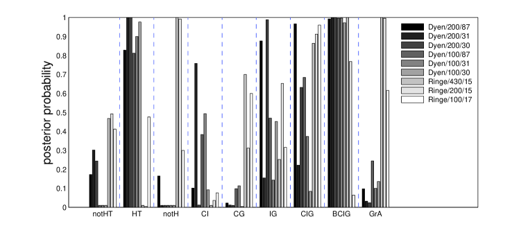
Figure 1: Posterior probabilites for selected clades, across data sets. $x$-axis labels: BGCI, Balto-Slav-Germanic-Celtic-Italic; GCI, Germanic-Celtic-Italic; CI, Celtic-Italic; CG, Celtic-Germanic; GI, Germanic-Italic; GrA, Greek-Armenian; $\sf notHT$, complement of Hittite-Tocharian; $\sf notH$, complement of Hittite.

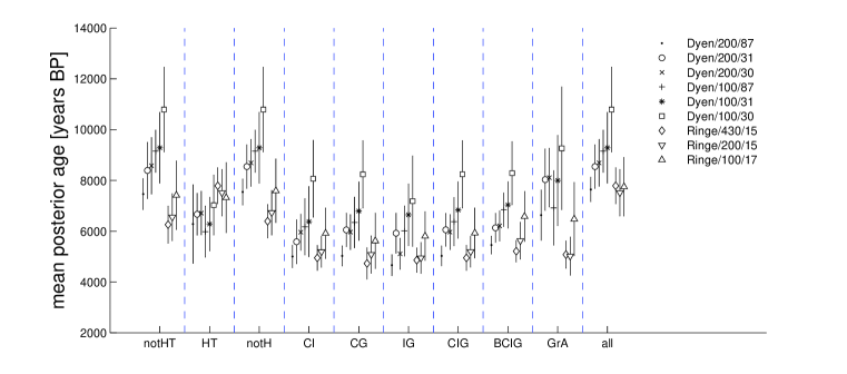
Figure 2: The mean posterior ages, in years BP, for the most recent common ancestor (MRCA, super-clade root) of languages in selected combinations of clades ($ie$ super-clades). $x$-axis labels as for Fig. 1.

In the supplement, Nicholls and Gray (2007), we define and display consensus trees, a central point estimate for topology and branch length. The consensus tree is not a state in the sample space of trees. Prior constraints and leaf ages are represented on sampled states so we give, in Figures 3 and 4, samples drawn from the ${\rm Dyen}/100/87$ and ${\rm Ringe}/100/17$ posterior distributions.

Referring to Fig. 1, there is some conflict in the support for clades across analyses. The BCIG group is strongly supported in all analyses (except ${\rm Ringe}/100/17$, which does at least allow it). The CIG group is supported in all analyses (except ${\rm Dyen}/100/30$, which allows it). However all the sub-clades CI, CG and IG are at odds with at least one data set. Age estimates for the common ancestor of the languages in the CIG clade are, in all analyses, close to the age estimates for the common ancestors of the subclades, suggesting the breakup occurred in a relatively small interval of time, so the split structure is poorly resolved.

Referring again to the clade probabilities, Fig. 1, and the consensus trees in the supplement, Hittite and Tocharian form an outgroup in the three ${\rm Dyen}/200/Y$ analyses, are grouped with Greek and Armenian in the ${\rm Dyen}/100/Y$ analyses, and are split in the three ${\rm Ringe}/X/Y$ analyses. There are many model mispecification issues for Hittite and Tocharian. Comparing notH and all in Fig. 2, Hittite adds 1000 years to the posterior mean root age in the ${\rm Ringe}/328/15$ analysis. The contrast between the Dyen et al. (1997) and Ringe et al. (2002) analyses is most clearly visible in the notH and notHT columns of Figures 1 and 2.

In contrast, conflicts between analyses of the Swadesh 100-word list (${\rm Dyen}/100/87$, ${\rm Dyen}/100/31$, ${\rm Dyen}/100/30$ and ${\rm Ringe}/100/17$, symbols $+*\Box\triangle$) are almost absent. Both CI and IG (see Fig. 1) are allowed by these analyses. ${\rm Ringe}/100/17$ allows the clade HT and does not impose HT as an outgroup (which would be a conflict, as notHT is not a clade of ${\rm Dyen}/100/Y$). In other areas of conflict, the ${\rm Dyen}/100/Y$ analyses allow a GrA clade. This lack of conflict comes at the price of greater random error (compared to analyses on longer word-lists). One striking conflict remains: the position of Indo-Iranian relative to the root is quite different in the ${\rm Ringe}/100/17$, and ${\rm Dyen}/100/Y$ analyses.

The posterior mean ages for the notH, notHT, all and GrA, which show particular conflict in Fig. 2, are in fair agreement for analyses based on the Swadesh 100-word list. Comparing the ${\rm Dyen}/100/30$ and ${\rm Ringe}/100/17$ analyses, and looking at Fig. 2 and Supplement-Fig. 7, the clade root ages for notHT do not agree in either simulation. Otherwise there is agreement between the four analyses, on the ten measured ages, under one or both prior weightings. This reduced ($K=100$) set of traits is chosen to be resistent to borrowing. Posterior predictive replicates computed in Section 9.3 show little evidence of rate heterogeneity within this class of traits. The corresponding words are relatively well attested in otherwise incompletely reconstructed ancient languages, so there is little missing data. In Section 9.2 we compute posterior predictive distributions for singleton traits in the ${\rm Ringe}/100/17$ analysis; these agree well with external data.

In summary, the systematic errors displayed in our four age estimates from the Swadesh 100-word list are representative. On the other hand, most features of tree topology which were in doubt, remain in doubt.

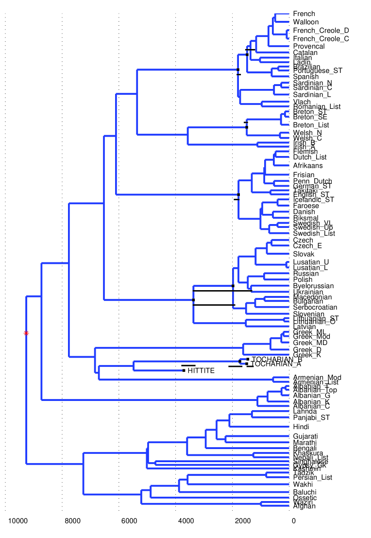
Figure 3: Tree sampled from the ${\rm Dyen}/100/87$ posterior distribution. $x$-axis gives age in years. Prior constraints on eight clade root and three leaf ages are indicated by horizontal bars. In order to reduce clutter, a single bar shows the two Tocharian A and B constraints, which are near equal.

Figure 4: A sampled state illustrating the ${\rm Ringe}/100/17$ posterior distribution. Prior constraints on topology impose 7 clades. Prior uncertainties in clade root and leaf ages are indicated by horizontal bars.

9 Model mis-specification

We head this section with a summary of its results. These results coincide with the conclusions we draw from the between-data analyses in Section 8.2: our age estimates are robust; tree topology less so. In Fig. 5 and Fig. 6 we present results from synthetic data, simulated on a tree sampled from the posterior distribution of the $Ringe/200/15$ analysis (true clade structure is marked in Fig. 5 with $0$ below false clades and $1$ below true; the true tree is in Nicholls and Gray (2007)), under a range of observation models intended to mimic likely model mis-specification. Details of these models, which simulate the empty-field-condition, plausible levels of borrowing and branch-wise and trait-wise rate heterogeneity, are given in Sections 9.1 through 9.7.

Clades imposed in reconstructions from synthetic data are indexed s- and are the same as the clades defined below Fig. 1 and displayed as horizontal bars in Fig. 4. Analyses of synthetic data are indexed “S/X/Y”. Values of X indicate borrowing and rate heterogeneity: X=“T” is no borrowing; X=“G$b$” is global borrowing at rate $b\mu$; X=“L$z-b$” is local borrowing, between languages with a common ancestor not more than $z$ years in the past, at rate $b\mu$; and X=“BH$\rho$” and X=“MH$\rho$” have rates drawn independently, for each branch (BH) and meaning category (MH) respectively, from a Gamma distribution with mean $\mu$ and standard deviation $(\rho/100)\mu$. Values of Y show the constraint applied: Y=“U$n$” is the unconstrained birth death process of set elements, with $n=\lambda/\mu$ the expected number of distinct traits at each leaf, under the NOABSENT observation model; Y=“C$n$” simulates cognate classes under the no-empty-field constraint, using $n$ meaning categories.

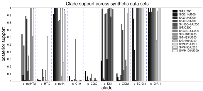
Figure 5: Synthetic data yields estimates of posterior probabilities for selected clades, across synthetic data sets. $x$-axis labels as for Fig. 1 with s- prefix indicating synthetic and 0/1 indicating absence/presence of the clade in the true tree.

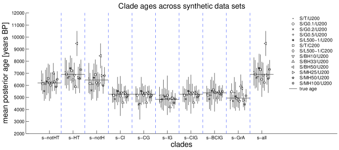
Figure 6: Synthetic data yields estimates of mean posterior ages, in years BP, for the most recent common ancestor (MRCA, super-clade root) as in Fig. 1 with s- prefix indicating synthetic.

Systematic errors in tree node ages inferred from synthetic data generated under these models are in general small. With the exception of $S/BH50/U200$ (see Section 9.4), the systematic error we generated in Fig. 6 is of the same order of magnitude as, or smaller than, random error. Systematic error in estimated rates $\mu$ (not shown) is highly significant. Calibration data fixes dates and topology for that part of the tree adjacent to the leaves, forcing the inference to accommodate model mis-specification by adjusting rates. The modified rates fit the imposed trait evolution adjacent to the leaves. If model mis-specification is homogeneous over the tree, as is the case for the empty-field-approximation, trait evolution deep in the tree may be well represented by these biased rates, and date estimates are accordingly robust.

Tree topology is not robust to the model mis-specification we explored. The “true” s-clades s-GrA, s-BCIG, and the rooting clades s-notHT, and s-notH have robust support at levels which do not allow rejection of the truth. The “true” s-clades s-CIG and s-IG are not well reconstructed when borrowing is substantial. The branching at the top of the superclade s-BCIG is poorly resolved as the s-BCIG, s-CIG and s-IG branches are separated by just 1000 years in the tree on which the synthetic data was simulated (see Nicholls and Gray (2007)), which is small compared to $\mu^{-1}\simeq 3000$. Nevertheless, the truth is rejected only at very high levels of borrowing (S/Gb/Y where $b=0.2,0.5$). Clade age estimates, shown in Fig. 2 and Fig. 6, can be stable across analyses when topology is uncertain. This is because the super-clade ages are determined largely by total tree length; total tree length is tightly coupled to the number of transitions on the tree, which is rather well determined by data.

9.1 Global and local borrowing

Word borrowing from languages outside the study is straightforward trait birth (unless the same word is borrowed into several languages). If we delete a source language from our study, we thereby remove the model error associated with borrowing from that language. The consistency we see in Fig. 2 between clade ages reconstructed for near-disjoint subsets of languages, and the full set, in the ${\rm Dyen}/200/87$, ${\rm Dyen}/200/31$ and ${\rm Dyen}/200/30$ posteriors, suggests that borrowing is not distorting the ${\rm Dyen}/200/87$ estimates themselves.

Our models of borrowing are as follows. We associate with each time slice $\tau\in[0,\infty)$ across the tree a linkage graph $({\cal E}(\tau),{\cal V}(\tau))$ with nodes, ${\cal V}(\tau)=\{(\tau,i);(\tau,i)\in[g]\}$, corresponding to points in $[g]$ intersected by the slice. The linkage graph models traffic between languages; its edges $\langle\,y,z\,\rangle\in{\cal E}(\tau)$ connect sets $H(y)$ and $H(z)$ between which trait instances can pass. Let $\tilde{\cal V}(z)=\{z\in{\cal V}(\tau):\exists y\in{\cal V}(\tau),\langle\,y,z\,\rangle\in{\cal E}(\tau)\}$ be the set of nodes adjacent to $z\in{\cal V}(\tau)$. Let $b$ denote the relative rate of word-borrowing to word-death. At per capita rate $b\mu$ each instance of each trait in each language in the time slice $\tau$ generates a borrowing event. Suppose the selected trait-instance is in language $z\in{\cal V}(\tau)$ and is labeled $c\in C$. A language $y\in\tilde{\cal V}(z)$ is chosen, uniformly at random from nodes adjacent to $z$ on $({\cal E}(\tau),{\cal V}(\tau))$, and we set $H(y)\leftarrow H(y)\cup\{c\}$, $ie$ the word is copied into the target language.

We model local borrowing as follows. Words transfer between languages which have a sufficiently recent common ancestor. The linkage graph at time $t$ includes an edge from $(t,i)$ to $(t,j)$ if points $(t,i)$ and $(t,j)$ in $[g]$ have a common ancestor less than $z$ years in the past. In this model linked groups of languages break up into linked subgroups. In our model of widespread borrowing (the “global” borrowing model), all languages communicate equally with all other languages, and the linkage graph is the complete graph.

Our exploration of these models is summarized in Figures 5 and 6 by the three S/G$b$/U200 data sets and the S/L$500-1$/U200 data set. We display global borrowing at relative rates of 10%, 20% and 50% the death rate. Higher global rates are probably irrelevant. In the data, the distribution of ${\rm card\,}(M_{a})$, the number of languages displaying cognate $a$, tails off rapidly, so that few cognates are displayed in many languages. At $b\simeq 1$, cognates simply survive too well, and many cognates from deep in the tree survive into many languages. Local borrowing has time depth $z=500$ and a borrowing rate equal to the death rate. We see from Fig. 6 that age estimates are robust to this form of model mis-specification.

9.2 Predictive distributions and external data

Where the observation model is NOABSENT, singleton traits are present, and we can use them to test the model. We drop them from the data, carry out the inference under NOUNIQUE, and then see if we can predict the number of singleton traits for each taxon. This check was available for the Ringe et al. (2002) data. We expect rate heterogeneity and borrowing to be visible (but probably not distinguishable) in these tests.

Denote by $\tilde{D}$ synthetic trait data generated under the NOABSENT observation model, displaying $\tilde{N}$ distinct traits. For trait $a=1,2,\ldots,\tilde{N}$ let $\tilde{M}_{a}$ give the indices of leaves displaying an instance of trait $a$ for predicted data $\tilde{D}$, and $\tilde{X}_{i}$ be the number of singleton traits in $\tilde{D}$ at taxon $i$,

$$\tilde{X}_{i}={\rm card\,}\{\tilde{M}_{a}:\tilde{M}_{a}=\{i\},a=1,2,\ldots,\tilde{N}\}\quad i\in V_{L}.$$

The posterior predictive distribution $\Pr\{\tilde{D}|D\}$ is

$$\Pr\{\tilde{D}|D\}=\int\Pr\{\tilde{D}|g,\mu,\lambda\}p(g,\mu,\lambda|D)dgd\mu d\lambda$$

and this determines a predictive distribution for $\tilde{X}_{i}$. We sample $\mu,\lambda$ and $g$ from the posterior $p(g,\mu,\lambda|D)$ ($g$ and $\mu$ are available from MCMC output; we restore $\lambda$ by sampling its posterior conditional density), simulate synthetic data $\tilde{D}$ at the leaves of $g$, and compute $\tilde{X}_{i}$ from $\tilde{D}$. Let $X_{i}(D)={\rm card\,}\{M_{a}:M_{a}=\{i\},a=1,2,\ldots,N\},$ denote the number of singleton traits at taxon $i$ in the original real data itself.

Predictive distributions for $X_{i}$ are given in Supplement-Fig. 9. The predictive distributions for $\tilde{X}_{i}$ over-estimate the $X_{i}$ in the Ringe et al. (2002) data with $K=328$ meaning categories. Since borrowing depletes singleton traits, this is consistent with model mis-specification due to borrowing. Also, we expect borrowing to be weaker on the shorter word-lists ($K=100,200$), since the shorter lists are by design more resistent to borrowing. We see in Supplement-Fig. 9 that singleton traits are indeed more reliably predicted on shorter lists (especially $K=100$). Rate heterogeneity can mimic this behavior. Corresponding studies for synthetic data are given in Supplement-Fig. 10,11. Predictive distributions from the shorter word-lists are in good agreement with the data.

9.3 Rate heterogeneity across traits

Pagel and Meade (2006) show that the evolution rates of words are, for a given meaning category, fairly consistent across data sets, whilst varying more substantially between meaning categories. Fig. 7 displays a tendency for the shorter word-lists to evolve at relatively slower rates. This is expected. However the rate variation between data sets in Fig. 7 does not lead directly to variation in estimated root times in Fig. 2. For example, ${\rm Dyen}/200/87$ and ${\rm Dyen}/100/87$ differ by a factor 1.5 in posterior mean rate, but by just 1.2 in root age. Time depth measurements do not depend on an assumption of constant rates between analyses, since rates are estimated from calibration points in the recent history of the same data used to predict branching times.

In order to generate synthetic data with rate heterogeneity across meaning classes (the $S/MH\rho/U200$ simulations), we draw rates

$$\mu^{(k)}\sim{\rm Gamma}(\alpha,\beta)$$

independently for each meaning category $k=1,2,\ldots,K$, with mean $\alpha\beta=\mu$ and variance $\alpha\beta^{2}=(r\mu)^{2}$, where $r=0.25,0.5$ and $r=1$, simulate a trait process $H^{(k)}(\tau,i)$ at rate $\lambda,\mu^{(k)}$, merge meaning categories, as Equation (11), and then read off data, as Equation (2). Pagel and Meade (2006) estimate that the rate variance over meaning classes is $(r\mu)^{2}\simeq\mu^{2}/9$.

Rate heterogeneity across traits distorts the distribution of the number, ${\rm card\,}M_{a}$, of languages in which trait $a\in C$ appears. Denote by $Y^{(n)}=Y^{(n)}(D)$ the number of traits displayed at $n$ leaves,

$$Y^{(n)}(D)={\rm card\,}\{M_{a}:{\rm card\,}M_{a}=n,a=1,2,\ldots,N\},$$

and let $\tilde{Y}^{(n)}=Y^{(n)}(\tilde{D})$ be the corresponding random variable computed from posterior predictive data $\tilde{D}\sim\Pr\{\tilde{D}|D\}$. We plot ${\sf E}(\tilde{Y}^{(n)}|D)-Y^{(n)}$ and the envelope $\pm 2{\rm std}(\tilde{Y}^{(n)}|D)$. In the supplementary material (Supplement-Fig. 12) we show that the fitting procedure is unable to reproduce the trait frequency distribution in synthetic data with high levels of rate heterogeneity across meaning classes (standard deviation $50\%$ of the mean) but lower levels ($25\%$) are invisible.

Returning to the real data, in Supplement-Fig. 13 (left), some inconsistency attributable to rate heterogeneity between traits is visible in our ${\rm Ringe}/328/15$ analysis. Among other problems, the data contains an excess of traits appearing in 10 or more leaves. This is caused by a small cohort of traits evolving at death rate $\mu$ small compared to the rest. The effect is very greatly reduced in the ${\rm Ringe}/100/17$ analysis (Supplement-Fig. 13, right). Analyses of the Dyen et al. (1997) data show a similar pattern.

9.4 Rate heterogeneity in space and time

Time depth measurements depend on some assumption about the way rates have changed over time within each data set we analyze. The variations in rates between clades within each of the D100, D200, R328 and R100 groups in Fig. 7 give us an indication of the un-modelled rate variation we can expect in the deeper branches of the tree.

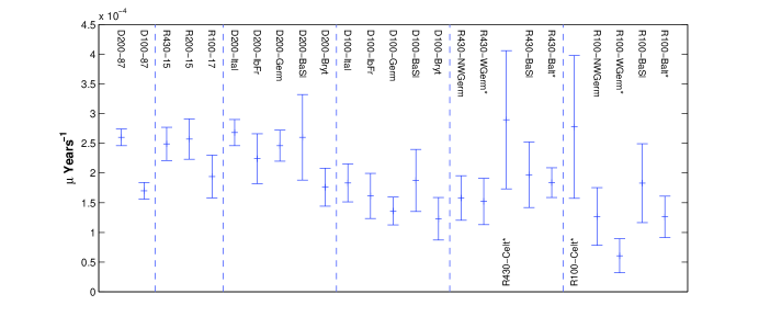
Figure 7: Posterior mean values of $\mu$, with standard errors at two standard deviations, measured in analyses ${\rm Dyen}/200/87$ (D200-87), ${\rm Dyen}/100/87$ (D100-87), ${\rm Ringe}/328/15$ (R328-15), ${\rm Ringe}/200/15$ (R200-15) and ${\rm Dyen}/100/17$ (R100-17), and independently using calibration points in distinct clades. The observation model is NOUNIQUE, except for two-leaf clades marked *, where NOABSENT must be used.

We give the per-trait-instance death rate $\mu$ for each clade calibration constraint independently. We sampled the posterior distributions $p(g,\mu|D_{\rm clade})$ determined by the data for each clade in turn. We could use the posterior rate distribution from one calibration clade as a prior to predict the age range for the root of another calibration clade. Where confidence intervals for the reconstructed rates of a given data set overlap, the corresponding predictions will be good. Such prediction is legitimate within one data set only, so we compare rates between vertical dashed lines.

In the supplement for this section we report and discuss a similar cross-validation exercise on the ${\rm Dyen}/100/87$ analysis. We drop each calibration-clade in turn (both topology and age constraint) and estimate the clade root age using all the word-list data and the remaining calibration points. Of 10 such tests, 8 succeed. The predicted age range for Balto-Slav is slightly too deep, and that of Hittite very significantly too young.

Synthetic data with spatio-temporal rate variation ($S/BH\rho/U200$ analyses), have rates

$$\mu_{\langle i,j\rangle}\sim{\rm Gamma}(\alpha,\beta)$$

drawn independently on each edge $\langle i,j\rangle\in E$, with mean $\alpha\beta=\mu$ and variance $\alpha\beta^{2}=(r\mu)^{2}$, where $r=\rho/100$, so that the standard deviation of the rates is 10%, 33% and 50% the mean rate. Lees (1953) sees 20% variation in rate estimates from pairs of languages. Results are robust to moderate levels of unstructured, random rate variation of this kind.

Results are of course not robust to structured rate variation, in which, for example, rates on edges at ages greater than any calibration point are all larger than any rates in the calibration zone, or a single-taxon outgroup has an extreme rate. In $S/BH50/U200$, $\sf s-hittite$ happens to have a high rate. Its root is pushed to great age, and with it goes the root of the tree. The analysis is exposed to rare “catastrophic” trait-evolution events outside the calibration zone. We checked that that no single language or small outgroup is determining the root age in the ${\rm Ringe}/100/17$, and ${\rm Dyen}/100/Y$ analyses. Agreement between reconstructions based on the predominantly ancient languages of Ringe et al. (2002) and modern languages of Dyen et al. (1997) shows that there is at least no such structured rate variation in the recent past.

9.5 The empty-field approximation

Our empty-field approximation will be good if there is significant “polymorphism”, that is, if the mean number $\lambda^{(k)}/\mu^{(k)}$ of traits ($ie$, words per meaning category) in the $H^{(k)}(\tau,i)$-process is large. We estimate $\lambda/\mu$ at $273(9)$ for the Dyen et al. (1997) Swadesh-200 data and $280(25)$ for the Ringe et al. (2002) Swadesh-200 data (posterior standard deviation in parenthesis) and hence $\lambda^{(k)}/\mu^{(k)}\simeq 1.4$. The probability, $\exp(-\lambda^{(k)}/\mu^{(k)})\simeq 1/4$, to find the unconstrained trait-set process $H^{(k)}(\tau,i)$ in the empty set at any single fixed point $(\tau,i)\in[g]$ is high enough to cause concern.

We simulate synthetic data from the trait birth-death process constrained to respect the no-empty-field condition. For each of the $k=1,2,\ldots,K$ meaning classes, we simulate $N^{(k)}(t_{R},R)$ from a Poisson distribution constrained to be greater than zero, then simulate $H^{(k)}(\tau,i)|N^{(k)}(\tau,i)>0$ in $[g]$. The total rate for the exponential waiting time to the next event does not include $\mu$ if $N^{(k)}(\tau,i)=1$. We then merge the meaning classes as in Equation (11). Our studies are represented here by two simulations, S/T/C200 and S/L500-1/C200, the latter including local borrowing. The per-capita death rate $\mu$ was set to a large value, so that polymorhpism was low. We find, when we fit data of this kind, that the tree and its dates are robust to this form of model mis-specification.

9.6 Incorrect splitting deep rooted homology classes

When the scientist groups instances of traits into homology classes, instances of traits born deep in the tree may be highly evolved, and correspondingly difficult to identify as in fact homologous. This error can populate the deeper branches of the tree with spurious birth events. This is a case where model mis-specification is not homogeneous over the tree, and will lead to over-estimation of the tree depth. When we replace the Ringe et al. (2002) “splitting” data with the Ringe et al. (2002) “lumping” data we do see a 3% downward shift in the estimated root time.

9.7 Unknown vocabulary as absent traits

In our analysis of the Ringe et al. (2002) data, we retain some languages with gaps, corresponding to missing data. We replace these gaps with zeros, marking trait absence. Gappy languages (Hittite, Tocharian) do stand out in predictive tests counting singleton traits on external data for the 328 and 200 word-lists. However, the effect is removed when we reduce the data to the Swadesh 100 word-list, where traits are better attested. The effect is to bias reconstructed branching times for gappy taxa to larger age values on the Ringe et al. (2002) 328 and 200 word-list data (see for example HT in Fig. 2).

References

- Atkinson et al. (2005) Atkinson, Q., G. Nicholls, D. Welch, and R. Gray (2005). From words to dates: water into wine, mathemagic or phylogenetic inference. Transactions of the Philological Society 103, 193–219.
- Bergsland and Vogt (1962) Bergsland, K. and H. Vogt (1962). On the validity of glottochronology. Current Anthropology 3, 115–153.
- Blust (2000) Blust, R. (2000). Why lexicostatistics doesn’t work: the “universal constant” hypothesis and the austronesian languages. In C. Renfrew, A. McMahon, and L. Trask (Eds.), Time depth in historical linguistics, pp. 311–332. Cambridge, UK: The McDonald Institute for Archaeological Research.
- Drummond et al. (2002) Drummond, A. J., G. K. Nicholls, A. G. Rodrigo, and W. Solomon (2002). Estimating mutation parameters, population history and genealogy simultaneously from temporally spaced sequnce data. Genetics 161, 1307–1320.
- Dyen et al. (1992) Dyen, I., J. Kruskal, and B. Black (1992). An Indoeuropean classification: a lexicostatistical experiment. Transactions of the American Philosophical Society 82(1-132).
-
Dyen
et al. (1997)
Dyen, I., J. Kruskal, and P. Black (1997).
Electronic format from website of 3rd author,
http://www.cdu.edu.au/research/profiles/profile_black.html - Embleton (1986) Embleton, S. (1986). Statistics in Historical Linguistics. Bochum: Brockmeyer.
- Erdem et al. (2006) Erdem, E., V. Lifschitz, and D. Ringe (2006). Temporal phylogenetic networks and logic programming. Theory and Practice of Logic Programming 6, 539–558.
- Felsenstein (1981) Felsenstein, J. (1981). Evolutionary trees from DNA sequences: a maximum likelihood approach. J. Mol. Evol. 17, 368–376.
- Felsenstein (1992) Felsenstein, J. (1992). Phylogenies from restriction sites: a maximum-likelihood approach. Evolution 46, 159–173.
- Garrett (2006) Garrett, A. (2006). Convergence in the formation of Indo-European subgroups: phylogeny and chronology. In P. Forster and C. Renfrew (Eds.), Phylogenetic Methods and the Prehistory of Languages, pp. 139–152. Cambride, UK: The McDonald Institute for Archaeological Research.
- Geyer (1992) Geyer, C. J. (1992). Practical Markov chain Monte Carlo (with discussion). Statist. Sci. 7, 473–511.
- Gray and Atkinson (2003) Gray, R. and Q. Atkinson (2003). Language-tree divergence times support the Anatolian theory of Indo-European origin. Nature 426, 435–439.
- Huson and Steel (2004) Huson, D. and M. Steel (2004). Phylogenetic trees based on gene content. Bioinformatics 20(13), 2044–2049.
- Kimura and Crow (1964) Kimura, M. and J. Crow (1964). The number of alleles that can be maintained in a finite population. Genetics 49, 725–738.
- Lees (1953) Lees, R. (1953). On the basis of glottochronology. Language 29, 113–127.
- Lewis (2001) Lewis, P. (2001). A likelihood approach to estimating phylogeny from discrete morphological character data. Systematic Biology 50, 913–925.
- Nakhleh et al. (2005) Nakhleh, L., D. Ringe, and T. Warnow (2005). Perfect phylogenetic networks: A new methodology for reconstructing the evolutionary history of natural languages. LANGUAGE, Journal of the Linguistic Society of America 81, 382–420.
-
Nicholls and
Gray (2007)
Nicholls, G. and R. Gray (2007).