Exploring the epsilon regime with twisted mass fermions

Abstract:

In this proceeding contribution we report on a first study in order to explore the so called $\epsilon$ regime with Wilson twisted mass (Wtm) fermions. To show the potential of this approach we give a preliminary determination of the chiral condensate.

PoS(LAT2007)084

1 Introduction

Simulations of lattice QCD in the so called $\epsilon$ regime [1] of the chiral expansion allow in principle the extraction of physical parameters, like decay constants and electroweak effective couplings. Simulations in the $\epsilon$ regime are not exclusive to lattice actions with exact lattice chiral symmetry. While topology certainly plays an important role in this extreme regime, here we aim at simulations which sample all the topological sectors. The motivation for this is that the original expressions are given for the situation where topology is summed over.

To fix the notation we recall that we use as the lattice action for $N_{\rm f}=2$ degenerate flavours

$$S[\chi,\overline{\chi},U]=S_{G}[U]+S_{F}[\chi,\overline{\chi},U],$$ (1)

where $S_{G}$ denotes the tree-level Symanzik improved gauge action [2]

$$S_{G}[U]=\frac{\beta}{3}\sum_{x}\left\{b_{0}\sum_{\mu<\nu}\mathbb{R}{\rm e}~{}{\rm{Tr}}\left[\mathbbm{1}-P^{(1\times 1)}(x;\mu,\nu)\right]+b_{1}\sum_{\mu\neq\nu}\mathbb{R}{\rm e}~{}{\rm{Tr}}\left[\mathbbm{1}-P^{(2\times 1)}(x;\mu,\nu)\right]\right\}$$ (2)

with the normalization condition $b_{0}=1-8b_{1}$, and $b_{1}=-{1\over 12}$. The fermionic part of the action is given by the Wtm action [3, 4]

$$S_{\rm F}[\chi,\overline{\chi},U]=a^{4}\sum_{x}\overline{\chi}(x)\Big{[}D_{\rm W}+i\mu_{\rm q}\gamma_{5}\tau^{3}\Big{]}\chi(x),$$ (3)

where

$$D_{\rm W}=\frac{1}{2}\{\gamma_{\mu}(\nabla_{\mu}+\nabla^{*}_{\mu})-a\nabla^{*}_{\mu}\nabla_{\mu}\}+m_{0},$$ (4)

$\nabla_{\mu}$, $\nabla^{*}_{\mu}$ are the standard gauge covariant forward and backward derivatives, $m_{0}$ and $\mu_{\rm q}$ are respectively the bare untwisted and twisted quark masses (for a recent review on Wtm and unexplained notations see ref. [5]).

The chiral phase diagram of Wilson-like lattice actions, due to lattice artefacts, is different from the one in the continuum [6, 7, 8]. In particular for our choice of the gauge and fermion action, the so called first order Sharpe-Singleton scenario [9] takes place. In this case at fixed lattice spacing $a$, if we set $m_{\rm PCAC}=0$ where

$$m_{\rm PCAC}=\frac{\sum_{\bf x}\langle\partial_{0}A_{0}^{a}(x)P^{a}(0)\rangle}{2\sum_{\bf x}\langle P^{a}(x)P^{a}(0)\rangle}\qquad a=1,2,$$ (5)

the values of the twisted mass which can be simulated, are bounded from below by a value $\mu_{\rm c}$ which is proportional to $a^{2}\Lambda_{\rm QCD}^{3}$ [10, 11, 12]. This result is obtained if one analyzes the potential of the chiral lagrangian describing the low energy properties of the theory taking into account also the cutoff effects of the lattice action up to O($a^{2}$). In particular this analysis is performed in infinite volume.

It is well known [1] that in continuum QCD if one sends the quark mass to zero keeping the size of the volume fixed, chiral symmetry is restored and no phase transition appears, i.e. the dependence of the chiral condensate on the quark mass is smooth. It is plausible to expect that at finite lattice spacing the same mechanism takes place, and in particular the critical point $\mu_{\rm c}$ smooths out. One way to show this is to include the effects of the non vanishing lattice spacing in the analysis of [1], and to study the mass dependence of the chiral condensate in the $\epsilon$ regime including the O($a^{2}$) effects. This work is currently in progress.

2 Algorithm

To simulate dynamical Wtm $N_{f}=2$ degenerate quarks in the $\epsilon$ regime, we propose to use a PHMC algorithm [13, 14, 15, 16]. We refer to these references for more details on the algorithm, and here we just shortly summarize the main ingredients. The expectation value of a generic observable ${\mathcal{O}}$ is given by

$$\langle{\mathcal{O}}\rangle=\frac{1}{{\mathcal{Z}}}\int{\mathcal{D}}[U]{\rm e}^{-S_{G}[U]}\det\left(QQ^{\dagger}\left[U\right]\right){\mathcal{O}}\left[U\right]\quad Q=\gamma_{5}\left[D_{\rm W}+i\mu_{\rm q}\gamma_{5}\right],$$ (6)

with $Q$ being a single flavour operator, which in the following is normalized to have the biggest eigenvalue equal to one. It can be computed splitting up the determinant in two terms

$$\det\left(QQ^{\dagger}\left[U\right]\right)=\frac{\det\left[QQ^{\dagger}P_{n,\tilde{\epsilon}}\left(QQ^{\dagger}\right)\right]}{\det\left[P_{n,\tilde{\epsilon}}\left(QQ^{\dagger}\right)\right]},\quad P_{n,\tilde{\epsilon}}\left(QQ^{\dagger}\right)\simeq\left[QQ^{\dagger}\right]^{-1},$$ (7)

where $P_{n,\tilde{\epsilon}}\left(QQ^{\dagger}\right)$ is a polynomial approximation of order $n$ for $\left[QQ^{\dagger}\right]^{-1}$ restricted in the region of the eigenvalue spectrum $[\tilde{\epsilon},1]$. The main idea is to split the eigenvalue spectrum of the Wtm operator into parts which are then treated by either incorporating them in the update step of a simulation algorithm or by taking them into account in a reweighting procedure. Following [13], and leaving out the stochastic estimate of the correction factor, the generic expectation value can be written as

$$\langle{\mathcal{O}}\rangle=\frac{\langle{\mathcal{O}}W\rangle_{P}}{\langle W\rangle_{P}},\quad W={\det\left[QQ^{\dagger}P_{n,\tilde{\epsilon}}\left(QQ^{\dagger}\right)\right]}\simeq\prod_{\lambda_{i}<\tilde{\epsilon}}\left[\lambda_{i}P_{n,\tilde{\epsilon}}\left(\lambda_{i}\right)\right],$$ (8)

and the reweighting factor $W$ is computed exactly evaluating $N_{\lambda}\simeq 20$ smallest eigenvalues of the Wtm operator where $\lambda_{i}$ denotes an eigenvalue of $QQ^{\dagger}$. This strategy should allow a better sampling of the configuration space, when the eigenvalues of the Wtm are particularly small. To be specific in the exploratory runs we have performed we have used a polynomial approximation with $n=380$ and a cutoff in the spectrum $\tilde{\epsilon}=5\cdot 10^{-5}$. The bare parameters used in the simulations are $\beta=3.9$, $a\mu_{\rm q}=5\cdot 10^{-4}$ and $\kappa=0.160856$ [17]. In fig. 1 we summarize first preliminary results concerning the quality of the runs.

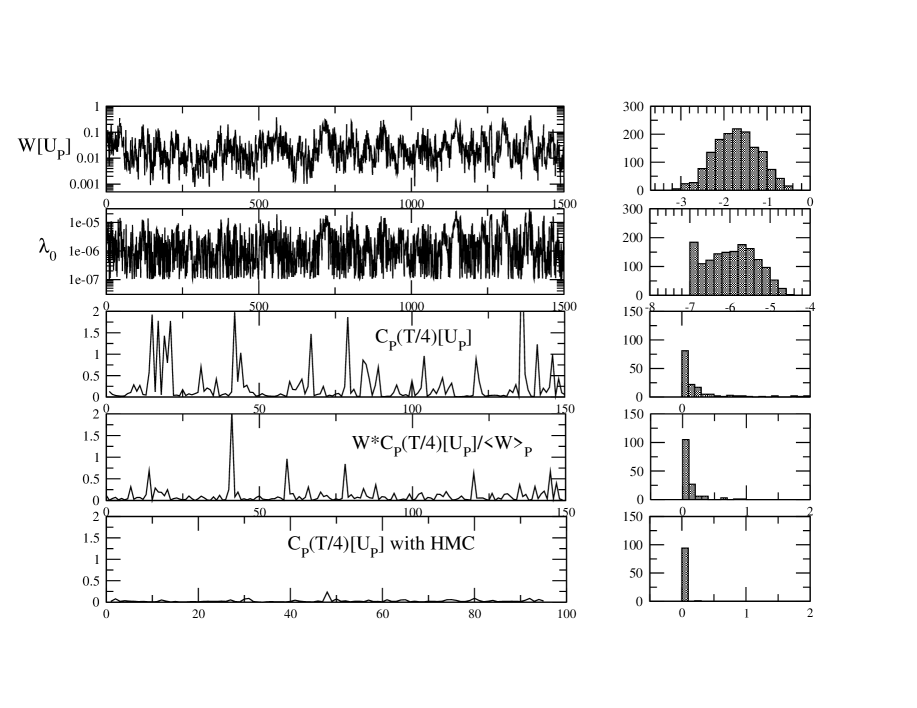
Figure 1: In the first stripe we plot the MC history and distribution of the reweighting factor $W$. In the second stripe we plot the MC history and distribution of the smallest eigenvalue $\lambda_{0}$ of $QQ^{\dagger}$. In the remaining three stripes we compare the MC histories and distributions of the pseudoscalar density correlator at time slice $x_{0}=T/4$ for the PHMC without and with reweighting factor and for the mt-mHMC.

In the first stripe we plot the MC history and distribution of the reweighting factor $W$. We observe a very smooth behaviour and a well behaved distribution. This has to be compared with the MC history and distribution of the smallest eigenvalue of $QQ^{\dagger}$, which is very small, but with fluctuations which are under control. In the remaining three stripes we compare the MC histories and distributions of the pseudoscalar density correlator (9) at time slice $x_{0}=T/4$ for the PHMC without and with reweighting factor and for the mass preconditioned HMC with multiple time scale integrator [18](mt-mHMC). This plot shows the different sampling of the configuration space by the two algorithms, and in particular the HMC seems to suppress contributions coming from the very low eigenvalues.These plots also show the expected advantages of the PHMC algorithm: better statistics for the large fluctuations and supression of exceptional fluctuations by the exact reweighting factor.

3 Sampling

To check that the algorithm correctly samples all the configuration space we have measured the topological charge $\nu$ using the field theoretical definition (proportional to $F\widetilde{F}$) on cooled and APE [19] or HYP [20] smeared gauge configurations. We emphasize that the aim of this exercise is just to have a first impression on how the algorithm is sampling the configuration space and it is not intended to be an attempt to compute physical quantities like the topological susceptibility.

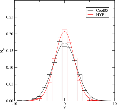
Figure 2: Distribution of the topological charge obtained with the field theoretical defintion on cooled and HYP smeared gauge configurations.

If we consider the sample of gauge configurations generated by the polynomial $P_{n,\tilde{\epsilon}}$ we obtain distributions of the topological charge as the ones in fig 2. In fig. 3 we compare the MC histories and distribution of the topological charge and of the minimal eigenvalue of $QQ^{\dagger}$ obtained with and without reweighting. We observe that the topological charge distribution $N_{\nu}$, after introducing the reweighting factor, has a qualitatively different shape.

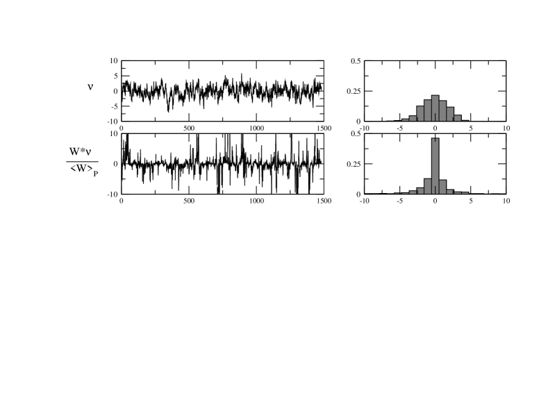
Figure 3: Comparison of the MC histories and distributions of the topological charge, obtained with one level of HYP smearing. We observe that the topological charge distribution $N_{\nu}$, after introducing the reweighting factor, has a qualitatively different shape, even if it shows that the algorithm is able to sample many topological sectors without any problem.

4 Results

A first preliminary result is given by the determination of the pseudoscalar density correlator

$$C_{P}(x_{0})=-a^{3}\sum_{\bf x}\langle P^{a}\left({\bf x},x_{0}\right)P^{a}\left(0\right)\rangle\quad a=1,2,$$ (9)

where

$$P^{a}\left(x\right)=\overline{\chi}(x)\gamma_{5}\frac{\tau^{a}}{2}\chi(x).$$ (10)

In the $\epsilon$ expansion we have a relation between the chiral condensate and $C_{P}(x_{0})$ [21, 22]. The equivalent relation at fixed topology can be found in [23]. The correlation function is expected to be constant up to a curvature in the Euclidean time given by the higher order corrections. In fig. 4 we show the Euclidean time dependence of the correlation $C_{P}(x_{0})$, with the fit result and range.

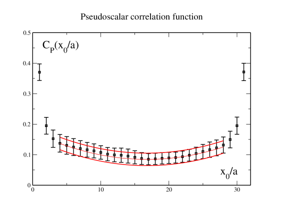
Figure 4: Dependence on $x_{0}/a$ of $C_{P}(x_{0})$ in the $\epsilon$ regime using Wtm fermions. A parabolic fit and the range used is also shown.

Inserting the values of the lattice spacing and renormalization factors

$$a=0.0855(5)(4),\qquad Z_{P}^{\overline{MS}}(\mu=2GeV)=0.46(1)(2)$$ (11)

computed by the ETMC [24, 25, 26] we obtain for the chiral condensate the following determination

$$|\Sigma_{\rm R}^{\overline{MS}}(\mu=2GeV)|=(264(12)(4)^{+20}_{-0}{\rm MeV})^{3}$$ (12)

where the first error is the summation in quadrature of all the statistical errors involved in the determination, the second error is an estimate of the systematic error coming from the error in the determination of $Z_{P}$, and the third is an estimate of the higher order corrections coming from the $\epsilon$ expansion.

This value compares nicely with the $p$ regime determination of ETMC [27] and of JLQCD [28] and other previous determinations summarized in tab.2 of ref. [29].

5 Outlooks

In this proceeding contribution we have shown that with Wtm fermions, simulations in the $\epsilon$ regime are feasible. It would be interesting to see if in the current simulations we have a physical volume which is big enough to perform a safe matching with chiral perturbation theory. Work on improving the basic PHMC algorithm we have used so far is in progress. Improvements on the quality of the correlation functions could be achieved with stochastic sources and low mode averaging. Interesting further investigations concern, e.g. the distribution of the topological charge, and the interplay between the chirally breaking O($a^{2}$) effects and the contribution of the zero modes to physical observables. Investigations in these directions are in progress.

References

- [1] J. Gasser and H. Leutwyler Phys. Lett. B188 (1987) 477.
- [2] P. Weisz Nucl. Phys. B212 (1983) 1.
- [3] ALPHA Collaboration, R. Frezzotti, P. A. Grassi, S. Sint and P. Weisz JHEP 08 (2001) 058 [hep-lat/0101001].
- [4] R. Frezzotti and G. C. Rossi JHEP 08 (2004) 007 [hep-lat/0306014].
- [5] A. Shindler arXiv:0707.4093 [hep-lat].
- [6] F. Farchioni et. al. Eur. Phys. J. C39 (2005) 421–433 [hep-lat/0406039].
- [7] F. Farchioni et. al. Eur. Phys. J. C42 (2005) 73–87 [hep-lat/0410031].
- [8] F. Farchioni et. al. Phys. Lett. B624 (2005) 324–333 [hep-lat/0506025].
- [9] S. R. Sharpe and J. Singleton, R. Phys. Rev. D58 (1998) 074501 [hep-lat/9804028].
- [10] G. Munster and C. Schmidt Europhys. Lett. 66 (2004) 652–656 [hep-lat/0311032].
- [11] S. R. Sharpe and J. M. S. Wu Phys. Rev. D70 (2004) 094029 [hep-lat/0407025].
- [12] L. Scorzato Eur. Phys. J. C37 (2004) 445–455 [hep-lat/0407023].
- [13] R. Frezzotti and K. Jansen Phys. Lett. B402 (1997) 328–334 [hep-lat/9702016].
- [14] R. Frezzotti and K. Jansen Nucl. Phys. B555 (1999) 395–431 [hep-lat/9808011].
- [15] R. Frezzotti and K. Jansen Nucl. Phys. B555 (1999) 432–453 [hep-lat/9808038].
- [16] T. Chiarappa, R. Frezzotti and C. Urbach hep-lat/0509154.
- [17] ETM Collaboration, P. Boucaud et. al. Phys. Lett. B650 (2007) 304–311 [hep-lat/0701012].
- [18] C. Urbach, K. Jansen, A. Shindler and U. Wenger Comput. Phys. Commun. 174 (2006) 87–98 [hep-lat/0506011].
- [19] APE Collaboration, M. Albanese et. al. Phys. Lett. B192 (1987) 163.
- [20] A. Hasenfratz and F. Knechtli Phys. Rev. D64 (2001) 034504 [hep-lat/0103029].
- [21] P. Hasenfratz and H. Leutwyler Nucl. Phys. B343 (1990) 241–284.
- [22] F. C. Hansen Nucl. Phys. B345 (1990) 685–708.
- [23] P. H. Damgaard, M. C. Diamantini, P. Hernandez and K. Jansen Nucl. Phys. B629 (2002) 445–478 [hep-lat/0112016].
- [24] C. Urbach PoS LAT2007 (2007) 022.
- [25] ETM Collaboration, P. Dimopoulos et. al. PoS LAT2007 (2007) 241.
- [26] ETM Collaboration, V. Lubicz, S. Simula and C. Tarantino PoS LAT2007 (2007) 374.
- [27] ETM Collaboration, P. Dimopoulos et. al. PoS LAT2007 (2007) 102.
- [28] H. Fukaya et. al. arXiv:0705.3322 [hep-lat].
- [29] C. McNeile Phys. Lett. B619 (2005) 124–128 [hep-lat/0504006].